Lyapunov vs. Geometrical Stability Analysis of the Kepler and the Restricted Three Body Problems

Abstract

In this letter we show that although the application of standard Lyapunov analysis predicts that completely integrable Kepler motion is unstable, the geometrical analysis of Horwitz et al [1] predicts the observed stability. This seems to us to provide evidence for both the incompleteness of the standard Lyapunov analysis and the strength of the geometrical analysis. Moreover, we apply this approach to the three body problem in which the third body is restricted to move on a circle of large radius which induces an adiabatic time dependent potential on the second body. This causes the second body to move in a very interesting and intricate but periodic trajectory; however, the standard Lyapunov analysis, as well as methods based on the parametric variation of curvature associated with the Jacobi metric, incorrectly predict chaotic behavior. The geometric approach predicts the correct stable motion in this case as well.

.1 I. Introduction

Several relatively recent papers have used geometric approaches to describe Hamiltonian chaos, implementing tools from Riemannian geometry PRE47 ; PRE48 ; PRE51 . The natural motions of Hamiltonian systems are viewed as geodesics on a Riemannian space associated with a metric $g_{ij}$ (often associated with either the Jacobi or the Eisenhart metric). Stable motions are thus defined by the curvature properties of the manifold.

Casetti et. al. PRE48 derived from the Jacobi–Levi-Civita (JLC) equation an effective stability equation which formally describes a stochastic oscillator. They conjectured that an “average” global geometric property should provide information about the  degree of chaos and applied the geometric method to the Fermi-Pasta-Ulam beta-model and to a chain of coupled oscillators.

Safaai and Saadat SafaaiSaadat have used the geometric method developed in PRE47 ; PRE48 ; PRE51 in an attempt to characterize the behaviour of the restricted three body problem in celestial mechanics. They conclude that the fluctuations of the curvature of the manifold along the geodesics yield parametric instability of the trajectories and are associated with chaos. They also calculated a positive Lyapunov exponent. We point out here that our simulation demonstrates stability for these orbits. We discuss the application of a recently developed geometrical criterion for stability to this problem, and show that it correctly predicts stability.

It has recently been shown Horwitz (to be called HBLSL) that there is a possibility to characterize instability in Hamiltonian systems by a geometrical approach which takes its point of origin in the curvature associated with a conformal Riemann metric tensor essentially different from the Jacobi metric, which is applicable to a large class of potential models (see also Li ). This approach appears to be more sensitive than computing Lyapunov exponents or the use of the Jacobi metric (see the book of Pettini PettiniBook for a review of important results obtained with methods related to the use of the Jacobi metric). This enables one to associate instability with a negative dynamical curvature appropriate for the geodesic motion different from that defined by the Jacobi metric, for which the line element is proportional to the time $t$  and not, as for the Jacobi metric, the action. This establishes a natural connection between chaotic Hamiltonian flows and Anosov flows Anosov directly in the time domain.

Additional problems in celestial mechanics can also be addressed with the HBLSL method, such as planetary stability and the Pioneer anomaly (see for example S. G. Turyshev and V.T. Toth Turyshev ).

.2  II. The Geometrical Method of HBLSL

In Horwitz the stability of a Hamiltonian system of the form (we use the summation convention)

$$H=\frac{\mathbf{p}^{2}}{2M}+V\left(x\right)=\frac{p^{i}p^{j}}{2M}\delta_{ij}+V\left(x\right)$$ (1)

was studied, where $V$ is a function of space variables alone, by introducing a second Hamiltonian of the type considered by Gutzwiller Jacobi ; Gutzwiller

$$H_{G}=\frac{1}{2M}g_{ij}p^{i}p^{j}$$ (2)

where $g_{ij}$ is a function of the coordinates alone. Hamilton’s equations applied to Eq. (2) result in the geodesic form

$$\ddot{x}_{l}=-\Gamma_{l}^{mn}\dot{x}_{m}\dot{x}_{n};$$ (3)

where

$$\Gamma_{l}^{mn}=\frac{1}{2}g_{lk}\{\frac{\partial g^{km}}{\partial x_{n}}+\frac{\partial g^{kn}}{\partial x_{m}}-\frac{\partial g^{nm}}{\partial x_{k}}\},$$ (4)

and $g^{ij}$ is the inverse of $g_{ij}$ .

Horwitz, et al Horwitz take $g_{ij}$ to be of conformal form

$$g_{ij}=\frac{E}{E-V\left(x\right)}\delta_{ij}$$ (5)

on the hypersurface defined by $H=E=constant$, resulting in a formal equivalence between the two Hamiltonians (1) and (2) on the same energy shell $E$.

The velocity field, defined by

$$\dot{x}^{j}\equiv g^{ji}\dot{x}_{i}=\frac{p^{j}}{M},$$ (6)

satisfies the geodesic equation

$$\ddot{x}^{l}=-\mathcal{M}_{mn}^{l}\dot{x}^{m}\dot{x}^{n}$$ (7)

where

$$\mathcal{M}_{mn}^{l}\equiv\frac{1}{2}g^{lk}\frac{\partial g_{nm}}{\partial x^{k}}.$$ (8)

The quantity (8) is a connection form, that is, it satisfies the requirements for the construction of a covariant derivative, but it is not compatible with the metric $g_{ij}$. It is therefore not a Christoffel symbol, but it may be derived as well by parallel transport on the Gutzwiller space and transformation to the coordinates $x^{j}$. The coordinates $x^{j}$ correspond to the manifold for which the velocity field is given by (6). This correspondence was discussed in Horwitz and will be discussed in more detail in HorwitzPrep .

It is shown in Horwitz that in the coordinates for which $g_{ij}$ has the form (5), Eq. (7) coincides with the Hamilton equations obtained from the Hamiltonian form (1), and thus provides a geometrical embedding of this Hamiltonian motion. The curvature associated with the connection form $\mathcal{M}$ is relevant to the dynamical stability of the Hamiltonian motion rather than the curvature associated with the connection form $\Gamma$ defined in (4). The geodesic deviation $\xi^{l}$ between two such orbits $x^{\prime}(t)$ and $x(t)$ satisfies

$$\frac{D_{\mathcal{M}}^{2}}{D_{\mathcal{M}}t^{2}}\xi^{l}=R_{\mathcal{M}qmn}^{l}\dot{x}^{q}\dot{x}^{n}\xi^{m},$$ (9)

where $\xi^{l}=x^{\prime l}(t)-x^{l}(t).$

Here, the covariant derivative of $\xi^{l}$ is defined by

$$\xi_{;n}^{l}=\frac{\partial\xi^{l}}{\partial x^{n}}+\mathcal{M}_{nm}^{l}\xi^{m}$$ (10)

and$\frac{D_{\mathcal{M}}}{D_{\mathcal{M}}t}$is the corresponding covariant derivative in$\ t$ along the instantaneously approximate common orbits, i.e.,

$$\frac{D_{\mathcal{M}}}{D_{\mathcal{M}}t}\xi^{l}=\dot{\xi}^{l}+\mathcal{M}_{nm}^{l}\dot{x}^{n}\xi^{m}.$$ (11)

What may be called the ’dynamical curvature’ appearing in (9) is given by

$$R_{\mathcal{M}qmn}^{l}=\frac{\partial\mathcal{M}_{qm}^{l}}{\partial x^{n}}-\frac{\partial\mathcal{M}_{qn}^{l}}{\partial x^{m}}+\mathcal{M}_{qm}^{k}\mathcal{M}_{nk}^{l}-\mathcal{M}_{qn}^{k}\mathcal{M}_{mk}^{l}.$$ (12)

With the conformal metric in noncovariant form (5), the geodesic deviation equation (9) becomes

$$\frac{D_{\mathcal{M}}^{2}}{D_{\mathcal{M}}t^{2}}\xi=-\mathcal{V}P\xi,$$ (13)

where the matrix $\mathcal{V}$ is given by

$$\mathcal{V}_{li}=\frac{3}{M^{2}v^{2}}\frac{\partial V}{\partial x^{l}}\frac{\partial V}{\partial x^{i}}+\frac{1}{M}\frac{\partial^{2}V}{\partial x^{l}\partial x^{i}}$$ (14)

and

$$P^{ij}=\delta^{ij}-\frac{v^{i}v^{j}}{v^{2}}$$ (15)

with $v^{i}=$ $\dot{x}^{i}$, defining a projection into a plane (in the two-dimensional examples we shall treat here, just a line) orthogonal to $v^{i}$.

Computer investigations Ben Zion of this local criterion show that local modifications of the Hamiltonian in regions where negative eigenvalues occur can be used to control the stability of the system. Removal or modification of the nonlinear and symmety breaking terms in just those local regions have dramatic effects on the Poincaré plots, completely stabilizing the global motion in the examples studied there.

It was argued in Horwitz that instability should occur if at least one of the eigenvalues of $\mathcal{V}$ is negative. This criterion was found to be effective for all of the examples we have studied Horwitz . Our experience with these examples indicates that positive eigenvalues are associated with stability. It is an interesting question, of course, to study whether there could be parametric instability associated with these positive eigenvalues (e.g.,PRE48 ). We remark that the investigations of SafaaiSaadat indicated a parametric instability in a system that was in fact stable, as our simulations show.

.3 III. Time Dependent Potentials

The analysis given above was carried out with a time independent potential function $V$. In order to analyze the stability of the restricted three body problem using the methods discussed in Section II, we first study the effect of a weak time dependence in $V$. In this case $E$ is not precisely conserved, but we shall make an adiabatic approximation in which we consider $E$ to be time independent. The time dependence of $V$ appears in the form of the geodesics generated by $H_{G}$ as an additional term with partial time derivative of the metric, but in the geometrical imbedding of the Hamiltonian motion, the geodesic evolution of the velocity vector field has the same form (7) as for the time independent potential problem. The formulation of geodesic deviation in terms of the second covariant derivative, however, as we shall see below, introduces another time derivative, introducing an additional term in the stability matrix. Referring back to the discussion of the previous Section, Eq.(9) is obtained by first computing $\ddot{\xi}^{l}$ with the help of (7). The resulting equation is simplified and rendered more transparent in its physical implication by re-expressing it in terms of the second covariant derivative. Although Eq.(7) is unaffected in form in the presence of a time dependence in $V$, the equation for the second covariant derivative, Eq.(9), now becomes

$$\frac{D_{\mathcal{M}}^{2}}{D_{\mathcal{M}}t^{2}}\xi^{l}=R_{\mathcal{M}qrp}^{l}\dot{x}^{q}\dot{x}^{p}\xi^{r}+\frac{\partial\mathcal{M}_{rp}^{l}}{\partial t}\dot{x}^{p}\xi^{r},$$ (16)

which is just Eq.(9) with the additional term

$$\frac{\partial\mathcal{M}_{rp}^{q}}{\partial t}\dot{x}^{p}\xi^{r}=\frac{1}{2}\frac{\partial^{2}g_{rp}}{\partial t\partial x_{q}}\dot{x}^{p}\xi^{r}$$ (17)

Using the conformal form of $g_{ij}$ with time dependent potential, the right hand side contains

$$\frac{\partial^{2}g_{rt}}{\partial x_{q}\partial t}=\ \ \ \ \ \ \ \ \ \ \ \ \ \ \ \ \ \ \ \ \ \ \ \ \ \ \ \ \ \ \ \ \ \ \ \ \ \ \ \ \ \ \ \ \ \ \ \ \ \ \ \ \ \ \ \ \ \ \ \ \ \ \ \ \ \ \ \ \ \ \ \$$

$$\left[\frac{2E}{\left(E-V\left(x,t\right)\right)^{3}}\frac{\partial V}{\partial t}\frac{\partial V}{\partial x_{q}}+\frac{E}{\left(E-V\left(x,t\right)\right)^{2}}\frac{\partial^{2}V}{\partial x_{q}\partial t}\right]\delta_{rt}$$ (18)

Near the boundary of the physical region, these terms can become large, but they are generally small away from these boundaries since they involve the time derivative of $V$, in the same approximation in which $E$ is constant (the consistency of this approximation will be discussed elsewhere). In our computations here these conditions hold, and we therefore compute stability using the same formulas as for the time independent problem. The modified Eq.(16) will be discussed in greater detail in a succeeding publication.

.4 IV. Application to Restricted Three Body Problem and Kepler Limit

We now consider the following Lagrangian of a restricted three body system:

$$L = T-V,\text{ \ \ \ }T=\frac{1}{2}m_{e}\left(\frac{d\vec{r}}{dt}\right)^{2}$$

$$V = \frac{1}{2}m_{j}r_{j}^{2}\omega_{j}^{2}-\frac{4\pi^{2}m_{e}}{r}-\frac{4\pi^{2}m_{j}}{r_{j}}-\frac{4\pi^{2}m_{e}m_{j}}{r_{ej}}.$$ (19)

In this system three bodies are involved: a large mass $M_{S}$ (the ”Sun”) at the origin (see Fig.LABEL:3bp1), a mass $m_{e}$ (”Earth”) located at $\vec{r}$, for which we study the trajectory, and a third mass $m_{j}$ (a ”Jupiter”) located at $\vec{r}_{j}$ circling the Sun,

$$\vec{r}_{j}=r_{j}(cos(\omega_{j}t),sin(\omega_{j}t)),$$ (20)

with $\omega_{j}$ and $r_{j}$ assumed to be constant (the first and third terms in $V$ are thus constant.). $r_{ej}$ denotes the distance between ”Earth” and ”Jupiter”. The time scale is in years, distances are in astronomical units and masses are scaled by the Sun mass. In these natural units $GM_{S}=4\pi^{2}.$

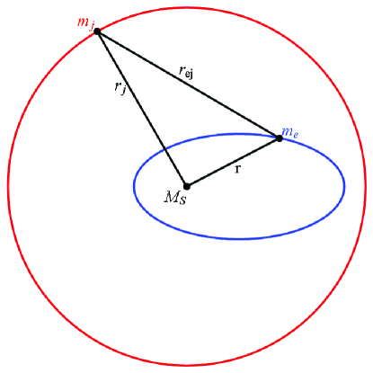
Figure 1: Depiction of the restricted three body problem.

We study the stability of the ’Earth’ trajectory using the standard Lyapunov analysis and also by the HBLSL geometrical approach. As shown in the Appendix the Lyapunov exponents depend on the eigenvalues of the matrix $\mathcal{V}^{HS}$ (which we shall call the Hamiltonian stability matrix)

$$\mathcal{V}_{kl}^{HS}=\frac{1}{m_{e}}\frac{\partial^{2}V}{\partial x_{k}\partial x_{l}},\text{ \ }k,l\in\{1,2\},\text{ \ }x_{1}\equiv x,\quad x_{2}\equiv y.$$ (21)

The standard Lyapunov eigenvalues $\lambda$ for the Hamiltonian motion (obtained, as usual, by reducing the set of the second order Newtonian equations to two sets of first order equations) are given by the square root of minus the eigenvalues of $\mathcal{V}^{HS}$ (which we denote by $\lambda_{HS}$), $\lambda=\pm\sqrt{-\lambda_{HS}}.$ Therefore, a positive eigenvalue for $\mathcal{V}^{HS}$ implies Lyapunov stability, and a negative eigenvalue implies Lyapunov instability (the resulting signs are therefore the opposite of the usual Lyapunov convention).

In the HBLSL geometrical approach we determine the stability of the trajectory by the eigenvalues of $\mathcal{V}$ in Eq.(14) which we rewrite as:

$$\mathcal{V}_{kl}=\frac{1}{m_{e}}\left[\frac{3}{2(E-V)}\frac{\partial V}{\partial x_{k}}\frac{\partial V}{\partial x_{l}}+\frac{\partial^{2}V}{\partial x_{k}\partial x_{l}}\right].$$ (22)

$E$ is now assumed to be adiabatically constant. By Eq.(13) a negative eigenvalue indicates an unstable trajectory while a positive eigenvalue indicates stability.

We study several cases distinguished in their ’Jupiter’ mass (the Kepler problem with zero Jupiter mass, the restricted Sun-Earth-Jupiter system with a ’regular’ Jupiter mass and a ’large Jupiter’) and in their ’Earth’ initial conditions (the latter leading to different eccentricities in the Kepler case). The planar motion that we analyze in these examples corresponds to the known planetary configurations; this enables us to reduce the problem to one with two coordinate degrees of freedom.

.4.1 The Kepler problem

Letting the Jupiter mass equal to zero, $m_{j}=0,$ we treat the classical Kepler problem. The Earth mass is taken as $m_{e}=2.96\cdot 10^{-6}.$ Three cases with different initial conditions are analyzed.

Circular orbit

A circular orbit is achieved by the initial conditions

$$\vec{r}(0)=(1,0),\quad\frac{d\vec{r}}{dt}|_{t=0}=(0,2\pi).$$ (23)

The eigenvalues of the Hamilton stability matrix $\mathcal{V}^{HS}$ are $-8\pi^{2}$ and $4\pi^{2},$ whereas the two eigenvalues of the HBLSL stability matrix $\mathcal{V}$ are both $4\pi^{2}$. Thus according to Lyapunov analysis the Kepler problem is unstable and could become chaotic. This is clearly a false result since the Kepler problem is integrable. (Of course, if one uses action-angle variables for the Kepler problem, it is predicted to be stable; we have used the Cartesian coordinates in order to illustrate that the Lyapunov method when applied without a careful choice of coordinates, not always available, may lead to an incorrect prediction Berry ). The geometrical HBLSL approach predicts stability of the orbit.

Realistic eccentricity

A more realistic orbit is obtained with the initial conditions

$$\vec{r}(0)=(1-e,0),\frac{d\vec{r}}{dt}|_{t=0}=(0,2\pi\sqrt{\frac{1+e}{1-e}}),e=0.0167,$$ (24)

where $e$ is the eccentricity of the Earth trajectory. One of the eigenvalues $\lambda_{HS}$ is again negative, oscillating  around its ’cicular’ value $-8\pi^{2}$, see Fig. 2, whereas the geometrical eigenvalues are both positive, showing oscillating deviations from their ’circular’ value $4\pi^{2}$ due to the small changes in the orbital radius. One of the eigenvalues is shown in Fig. 3, with the negative deviations, whereas the second eigenvalue bears positive deviations.

Figure 2: The eigenvalue of the Hamilton stability matrix Eq.(21) as a function of time for Kepler problem, $m_{j}=0,$ with initial conditions (24). Note that for the circular orbit the HS eigenvalue is $-8\pi^{2}.$

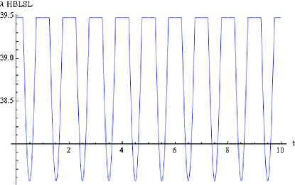
Figure 3: The eigenvalue of the HBLSL stability matrix Eq.(22) as a function of time for the Kepler problem, $m_{j}=0,$ with initial conditions (24). Note that for the circular orbit the HBLSL eigenvalue is $4\pi^{2}.$

Comparison with Ref.SafaaiSaadat

In order to compare our results with those of SafaaiSaadat we used the same initial conditions:

$$\vec{r}(0)=(1,0),\frac{d\vec{r}}{dt}|_{t=0}=(0,1).$$ (25)

The small initial velocity causes a large ’eccentricity’ in the ellipse-like trajectory, which allows us to elucidate the question of stability. We remark that the initial conditions that we have chosen, Eq.(24), take into account explicitly the eccentricity of the elliptic orbit. The computations of SafaaiSaadat used a shifted $x$ coordinate and a $y$ coordinate scaled by $2\pi$. The trajectory of the ’Earth’ is depicted in Fig.4.

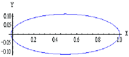
Figure 4: The Kepler orbit ($m_{j}=0)$ with initial conditions (25).

Fig. 5 reveals that one of the Hamiltonian stability eigenvalues is indeed negative along the entire orbit although its negative value is less pronounced between perihelia than at the perihelia.

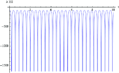
Figure 5: The eigenvalue of the Hamilton stability matrix Eq.(21) as a function of time for the Kepler problem with initial conditions (25)

Yet the geometric HBLSL eigenvalue, depicted in Fig. 6 as a function of time, is found to be positive in between perihelia, hence the trajectory is predicted to be globally stable. The trajectory only spends a short time at the unstable perihelia; this instability appears not to have an effect on the behaviour of the orbit globally in this case. We infer that if such local regions of negative eigenvalue are traversed in sufficiently short time, or have sufficiently small extension, global instabilities will not be observed (we are currently investigating this effect). This is a clear indication that the geometrical HBLSL analysis is preferable.

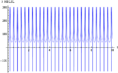
Figure 6: The eigenvalue of the HBLSL stability matrix Eq.(22) for the restricted three body problem with $m_{j}=m_{j0}$ with initial conditions (25).

.4.2 The restricted three body problem

The actual Jupiter mass

In the second case we study we use the ’regular’ Jupiter mass $m_{j0}=317.9$ $m_{e}=9.41\cdot 10^{-4},$ the mean Jupiter-Sun distance $r_{j}=5.203,$ and the Jupiter orbital period of $11.86$ years.

Applying the initial conditions Eq.(24) that lead to the realistic eccentricity in the Kepler case) we find that the Earth orbit is not altered by the ’added’ Jupiter. This is also true for the eigenvalues depitcted in Figs.7 and 8. A minute oscillation of a 24 year period due to Jupiter is apparent.

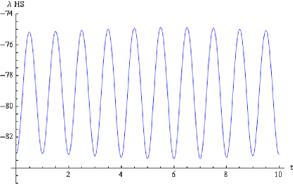
Figure 7: The eigenvalue of the Hamilton stability matrix Eq.(21) for the restricted three body problem with $m_{j}=m_{j0}$ with initial conditions (24).

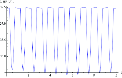
Figure 8: The eigenvalue of the HBLSL stability matrix Eq.(22) for the restricted three body problem with $m_{j}=m_{j0}$ with initial conditions (24).

While employing the initial conditions of SafaaiSaadat the ’added’ Jupiter does also not visibly modify the orbit and the eigenvalues as compared with the relevant Kepler case.

A large Jupiter

The third case deals with a ’large Jupiter’, $m_{j}=1000m_{j0}.$ (We remark that this value is close to the mass of the Sun, and therefore the dynamics is close to that of a binary solar system. We shall discuss this point further elsewhere.)

Again applying the initial conditions $\vec{r}(0)=(1-e,0),$ $\frac{d\vec{r}}{dt}|_{t=0}=(0,2\pi\sqrt{\frac{1+e}{1-e}})$ results in a knotty, yet periodic trajectory, shown in Fig 9. The Hamilton stability eigenvalue is again always negative along the orbit, depicted in Fig. 10, while the HBLSL geometric eigenvalue along the orbits, Fig. 11, is mainly positive with short negative excursions, similar to the Kepler case discussed above.

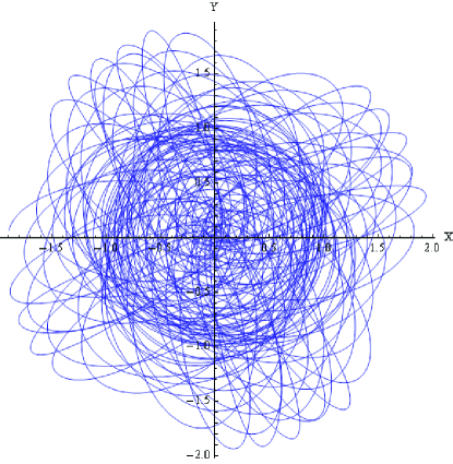
Figure 9: The earth orbit for the restricted three body problem with $m_{j}=1000m_{j0}\$during 100 time units with the initial conditions Eq.(24).

Figure 10: The eigenvalue of the Hamilton stability matrix Eq.(21) as a function of time for the restricted three body problem with $m_{j}=1000m_{j0}$ and initial conditions (24).

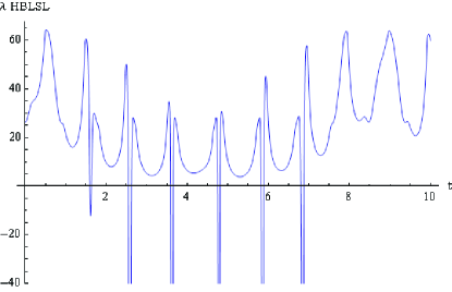
Figure 11: The eigenvalue of the HBLSL stability matrix Eq.(22) as a function of time for the restricted three body problem with $m_{j}=1000m_{j0}$ with initial conditions (24).

The initial conditions of SafaaiSaadat with the ’large Jupiter’ create a complicated, but clearly periodic ’Earth’ trajectory, Fig. 12. The eigenvalues are given in Figs. 13 and 14. The same conclusions are obtained: Lyapunov analysis predicts instability and possible chaos, while the geometrical HBLSL analysis predicts stability.

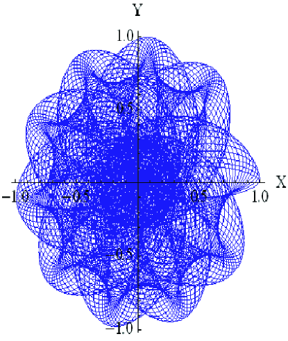
Figure 12: The earth orbit for the restricted three body problem with $m_{j}=1000m_{j0}\$during 100 time units with initial conditions (25).

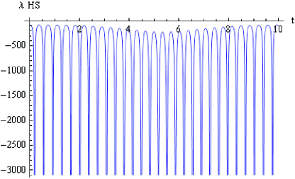
Figure 13: The eigenvalue of the Hamilton stability matrix Eq.(21) as a function of time for the restricted three body problem with $m_{j}=1000m_{j0}$ with initial conditions (25).

Figure 14: The eigenvalue of the HBLSL stability matrix Eq.(22) as a function of time for the restricted three body problem with $m_{j}=1000m_{j0}$ with initial conditions (25).

The application by Safaai et. al. SafaaiSaadat of the methods of Casetti and Pettini using the criterion of stability under parametric oscillations (see ref.PettiniBook ) also appear to predict chaotic behaviour, which is not in agreement with our simulations.

.5 V. Conclusions

The Lyapunov method for testing stability of Hamiltonian motion, as well as the parametric oscillator extensions of the Jacobi metric criteria PRE47 ; PRE48 ; PRE51 ; PettiniBook are not effective for the case of the restricted three body problem. The Lyapunov procedure, involving a linearization of the equations of motion in the neighborhood of a point on the orbit, does not take into account the curvature of the surface on which the system evolves, and we conjecture that this is the reason that the Lyapunov criterion is ineffective in certain applications. Moreover, the use of the Jacobi metric to define the geometry may also be weakened in its effectiveness, since the invariant interval is the action rather than the actual time; as pointed out in ref.PRE48 , the transformation changing the parameter along the orbit from action to time has the effect of essentially removing the geometrical embedding. This indicates, as for the Lyapunov computation, that the curvature of the surface on which the motion evolves may not be, in certain cases, sufficiently taken into account. The HBSL method provides an embedding of the Hamiltonian motion in a geometrical framework that appears to properly take into account the curvature of the surface on which the motion evolves in the actual laboratory time.

The HBSL method correctly predicts the stability of the restricted three body system. Moreover, the application of the Lyapunov method to the case $m_{j}\rightarrow 0$, the two body Kepler problem, predicts instability, whereas the HBLSL criterion is consistent with stability. We remark that there are clearly cases where adiabatic perturbation can result in strong chaos Elskens . In our analysis, for Hamiltonian systems, even if the Hamiltonian function is constant to a good approximation, the contribution given by (18) could have a large effect if the system approaches physical boundaries, such as could happen in the problem, for example, of the Duffing oscillator which has a hyperbolic fixed point. This does not occur in the case we are studying here. The effects of (18) when it is not negligible are under study.

We further remark that the form (19) can be easily generalized to treat the effect of several (unperturbed) planets on the motion of the two body subsystem, and the method can therefore be extended to a wider class of problems in celestial mechanics (as well as satellite motion).

We conclude, with this application and others previously treated Horwitz ; Li that the recently discovered HBLSL criterion is a powerful and useful tool for the analysis of the stability of Hamiltonian systems.

Acknowledgements. We thank the referees for a careful reading of the manuscript and their helpful comments. We are indebted to M. Schiffer, E. Kalderon and S. Shnider for valuable discussions.

I Appendix

The Newtonian equation of motions are

$$\ddot{x}_{i}=-\frac{\partial V\left(x\right)}{\partial x_{i}}$$ (A1)

Substituting $y_{i}=\dot{x}_{i}$ results in a system of two first-order equations for each degree of freedom $i$

Consider a new set of variables which are functions of the $x_{i}$ and $y_{i}$,

$$q_{k}=q_{k}\left(x_{i},y_{i}\right).$$

Expanding $q_{k}$ at $r_{j}+\delta r_{j}$, where the $r_{j}$ denote $x_{i},y_{i},$

$$q_{k}+\delta q_{k}=q_{k}\left(r_{j}+\delta r_{j}\right)=q_{k}\left(r_{j}\right)+\frac{\partial q_{k}}{\partial r_{j}}\delta r_{j}$$

and differentiating in time: $\dot{q}_{k}+\delta\dot{q}_{k}=\dot{q}_{k}\left(r_{j}+\delta r_{j}\right)=\dot{q}_{k}\left(r_{j}\right)+\frac{\partial\dot{q}_{k}}{\partial r_{j}}\delta r_{j}$ gives

$$\delta\dot{q}_{k}=\frac{\partial\dot{q}_{k}}{\partial r_{j}}\delta r_{j}$$

Explicitly

$$\left(\begin{array}[]{c}\delta\dot{x}_{1}\\ \delta\dot{x}_{2}\\ \delta\dot{y}_{1}\\ \delta\dot{y}_{2}\end{array}\right)=\left(\begin{array}[]{cccc}0&0&1&0\\ 0&0&0&1\\ -V_{11}&-V_{12}&0&0\\ -V_{12}&-V_{22}&0&0\end{array}\right)\left(\begin{array}[]{c}\delta x_{1}\\ \delta x_{2}\\ \delta y_{1}\\ \delta y_{2}\end{array}\right)$$ (A3)

where $V_{ij}\equiv\frac{\partial^{2}V}{\partial x_{i}\partial x_{j}}.$ The eigenvalues (here $\lambda$ is the standard Lyapunov eigenvalue) are given by the roots of

$$\lambda^{4}+\lambda^{2}\left(V_{11}+V_{22}\right)+\left(V_{11}V_{22}-V_{12}^{2}\right)=0$$ (A4)

Compare these eigenvalues to those of the Hamiltonian stability matrix $\mathcal{V}^{HS}=\left(V_{ij}\right),$ Eq.(21),

$$\left|\begin{array}[]{cc}V_{11}-\lambda_{HS}&V_{12}\\ V_{12}&V_{22}-\lambda_{HS}\end{array}\right|=0$$ (A5)

Hence

$$\lambda_{HS}^{2}-\lambda_{HS}\left(V_{11}+V_{22}\right)+\left(V_{11}V_{22}-V_{12}^{2}\right)=0$$ (A6)

With $\lambda_{HS}$ replaced by $-\lambda^{2}$ Eq.(A6) becomes equivalent to Eq.(A4), so that $\lambda_{HS}=-\lambda^{2}$.

The stability conditions are

$$\begin{array}[]{c}\lambda_{HS}>0,\ \ \ \ \ \lambda^{2}<0\ \ \ \rightarrow\ \ \ \ \ \text{stable}\\ \lambda_{HS}<0,\ \ \ \ \ \lambda^{2}>0\ \ \ \rightarrow\ \ \ \ \ \text{unstable}\end{array}$$ (A7)

Hence in our notation, positive eigenvalues of $\frac{\partial^{2}V}{\partial x_{i}\partial x_{j}}$ result in Lyapunov stability, negative eigenvalues of $\frac{\partial^{2}V}{\partial x_{i}\partial x_{j}}$ result in Lyapunov instability.

References

- (1) M. Pettini, Phys. Rev. E 47, 828 (1993).
- (2) L. Casetti and M. Pettini, Phys. Rev. E 48, 4320 (1993).
- (3) M. Ceruti-Sola and M. Pettini, Phys. Rev. E 51, 53 (1994).
- (4) H. Safaai, M. Hasan and G. Saadat, Understanding Complex Systems (Springer Berlin, 2006).
- (5) L.Horwitz, Y. Ben Zion, M. Lewkowicz, M. Schiffer and J. Levitan, Phys. Rev. Lett, 98, 234301 (2007). See also Y. Ben Zion and L. Horwitz, Phys. Rev. E 76, 046220 (2007); Y. Ben Zion and L. Horwitz, Phys. Rev. E 78, 036206 (2008).
- (6) J. Li and S. Zhang, J. Phys. A: Math. Theor. 43, 125105 (2010).
- (7) M. Pettini, Geometry and Topology in Hamiltonian Dynamics and Statistical Mechanics, Springer Verlag, New York (2007).
- (8) D. Anosov, Geodesic flows on closed Riemannian manifolds with negative curvature, Proc Steklov Instit. Math. 90, Amer. Math. Soc. Providence, Rhode Island, 1969.
- (9) S.G. Turyshev and V.T. Toth, to be published in Living Reviews in Relativity (2010), arXiv:1001.3686.
- (10) C.G.J. Jacobi, Vorlesungen über Dynamik, Verlag G. Reiner, Berlin (1844); J.S.Hadamard, J. Math. Pures et Appl. 4, 27 (1898).
- (11) M.C. Gutzwiller, Chaos in Classical and Quantum Mechanics, Springer-Verlag, New York (1990). See also W.D. Curtis and F.R. Miller, Differentiable Manifolds and Theoretical Physics, Academic Press, New York (1985), J. Moser and E.J. Zehnder, Notes on Dynamical Systems, Amer. Math. Soc., Providence (2005), and L.P. Eisenhardt, A Treatise on the Differential Geometry of Curves and Surfaces, Ginn, Boston (1909) [Dover, N.Y. (2004)].
- (12) L.Horwitz, A. Yahalom, J. Levitan, and M. Lewkowicz, Hamiltonian Mechanics on Geometrically Dual Manifolds, in preparation; see also E. Kalderon, S. Shnider and L.P. Horwitz, On a geometrical characterization of chaos in Hamiltonian dynamics, in preparation.
- (13) Y. Ben Zion and L. Horwitz, Controlling Effect of Geometrically Defined Local Structural Changes on Chaotic Systems, Phys. Rev. E 81, 046217 (2010); arXiv:1002.0142.
- (14) We wish to thank Michael Berry for bringing this point to our attention.
- (15) Y. Elskens and D.F. Escande, Nonlinearity 4, 615 (1991); A.I. Neishtadt, V.V. Sigorenko and D.V. Treschev, Chaos 7, 2 (1997); A. Neishtadt and A. Vasiliev, Chaos 17, 043104 (2007).