School of Science, East China University of Science and Technology, Shanghai 200237, China
Research Center for Econophysics, East China University of Science and Technology, Shanghai 200237, China
Research Center on Fictitious Economics & Data Science, Chinese Academy of Sciences, Beijing 100080, China
Economics; econophysics, financial markets, business and management Systems obeying scaling laws Fractals Self-organized systems
The components of empirical multifractality in financial returns
Abstract
We perform a systematic investigation on the components of the empirical multifractality of financial returns using the daily data of Dow Jones Industrial Average from 26 May 1896 to 27 April 2007 as an example. The temporal structure and fat-tailed distribution of the returns are considered as possible influence factors. The multifractal spectrum of the original return series is compared with those of four kinds of surrogate data: (1) shuffled data that contain no temporal correlation but have the same distribution, (2) surrogate data in which any nonlinear correlation is removed but the distribution and linear correlation are preserved, (3) surrogate data in which large positive and negative returns are replaced with small values, and (4) surrogate data generated from alternative fat-tailed distributions with the temporal correlation preserved. We find that all these factors have influence on the multifractal spectrum. We also find that the temporal structure (linear or nonlinear) has minor impact on the singularity width of the multifractal spectrum while the fat tails have major impact on , which confirms the earlier results. In addition, the linear correlation is found to have only a horizontal translation effect on the multifractal spectrum in which the distance is approximately equal to the difference between its DFA scaling exponent and 0.5. Our method can also be applied to other financial or physical variables and other multifractal formalisms.
pacs:
89.65.Ghpacs:
89.75.Dapacs:
05.45.Dfpacs:
05.65.+b1 Introduction
There are a wealth of studies showing that financial markets exhibit multifractal nature [1, 2, 3]. Many different methods have been applied to characterize the hidden multifractal behavior in finance, for instance, the fluctuation scaling analysis [4, 5, 6], the structure function (or height-height correlation function) method [1, 7, 8, 9, 10, 11, 12, 13, 14, 15, 16, 17], the multiplier method [18], the multifractal detrended fluctuation analysis (MF-DFA) [19, 20, 21, 22, 23, 24, 25, 26, 27], the partition function method [28, 29, 30, 31, 32, 33, 34, 35, 36, 37, 38], the wavelet transform approaches [39, 40, 41, 42], to list a few. There are also efforts seeking for applications of the extracted multifractal spectra. Some researchers reported that the observed multifractal singularity spectrum has predictive power for price fluctuations [29, 31, 38], can serve as a measure of market risk by introducing a new concept termed multifractal volatility [35], and can be used to quantify the inefficiency of markets [43].
An important and subtle issue of multifractality is about its origin. An even critical question is to ask whether the extracted multifractality is intrinsic or apparent. Indeed, it has been shown that an exact monofractal financial model can lead to an artificial multifractal behavior [44]. It is usually argued in the Econophysics community that the sources of multifractal nature in financial time series are the fat tails and/or the long-range temporal correlation [19]. However, possessing long memory is not sufficient for the presence of multifractality and one has to have a nonlinear process with long-memory in order to have multifractality [45]. In many cases, the null hypothesis that the reported multifractal nature is stemmed from the large price fluctuations cannot be rejected [46].
In this Letter, we focus on the multifractal detrended fluctuation analysis of financial logarithmic returns defined as
| (1) |
where is the price at time . Specifically, we use the daily data of the Dow Jones Industrial Average (DJIA) from 26 May 1896 to 27 April 2007 (totally 30147 trading days) to illustrate the method and results. The reason is simply that most studies in this direction use MF-DFA on stock returns. Nevertheless, the methodology is quite general and also applies in the study of other financial variables and other multifractal analysis.
The most studied factor is the temporal correlation in the return series, where the singularity spectrum of the real data is compared with that of the randomly shuffled data [20, 42, 22, 21, 47, 48]. All these studies show that the shuffled data have non-shrinking singularity width and the vertex with may shift left more or less. These observations imply that the heavy-tailed distribution of the returns has crucial impact on the singularity width. Extensive numerical experiments using uncorrelated time series obeying -Gaussian distributions with different tail exponents unveil a convergence to monofractalilty in the Gaussian attraction basin and to bifractality in the Lévy attraction basin [49], which is consistent with the analytic derivation of truncated Lévy flights [50]. Similar phenomena are observed for exponential distributions in the partition function framework [51]. To understand the impact of the distribution, one can either remove the large positive and negative returns [52] or generate surrogate data having a Gaussian distribution while keeping the linear correlation of the original data [53, 26, 27]. In this Letter, we will systematically investigate these factors together with a new factor reflecting possible hidden patterns in the raw time series.
2 Memory effect
We adopt the MF-DFA method to obtain empirically the singularities and the corresponding spectrum for each time series [19]. In all the cases, the scaling range of the detrended fluctuation function with respect to the time scale is , the moment order varies from -5 to 5, and the second-order polynomial (parabolic) is used for detrending.The determination of the scaling range is a subtle issue since the intrinsic scaling behavior will be masked or deformed by high-order trends or nonlinearity [54, 55, 56]. The power laws of the detrended fluctuation functions are not perfect. However, we find that the resulting multifractal spectra do not change much when we using a much narrower scaling range . When the time scale is 3000, there are only 20 boxes from both ends of the time series. To gain better statistics, we modify slightly the MF-DFA algorithm in the partitioning of boxes for a given time scale. Consider a time series . For time scale , we select a random sequence , which are uniformly distributed in . In our analysis, we use . This sequence determines boxes , in which the locally detrended fluctuation functions are calculated. If the time series is long-term power-law correlated, scales as a power law of [19]
| (2) |
The mass scaling exponent in the partition function formulism can be determined as
| (3) |
and the singularity strength and its spectrum can be calculated according to the Legendre transform [57]
| (4) |
The multifractal spectrum of the return series is thus determined and shown in fig. 1. We then shuffle the return series 100 times and determine their singularity spectra . For each point on the curve of the shuffled data, and are the arithmetic averages of the respective 100 values of the shuffled data and the error bar is the corresponding standard deviation. The singularity width is for the original data and for the shuffled data. These results are consistent with previous works. We also observe that the surrogate data have negative dimensions for larger , which implies that the surrogate data contains more randomness in large values of local detrended fluctuations [58, 59].
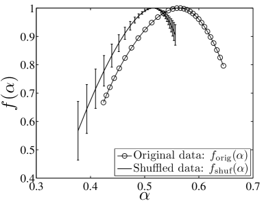
3 Effect of distribution
As we have shown above that, shuffling the return time series does not eliminate its multifractality. This is not surprising since there is no (or very weak) long-term correlation in the returns. Since the shuffled time series still exhibits a wide singularity spectrum, it is natural to conjecture that the distribution of returns has essential impact on the curve. We try to systematically test this conjecture using surrogate data. Two methods are adopted to generate surrogate data. One method is to replace the returns having large magnitudes with random numbers drawn from a normal distribution [52]. The other method is to substitute the raw returns with data drawn from prescribed distributions by keeping the ranking order which is relevant to the phase randomization algorithm [60] but with some differences.
3.1 The truncation method
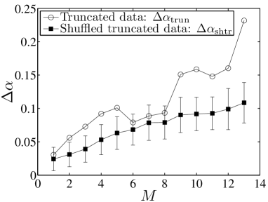
The truncation method was originally proposed to study the impact of large positive and negative values on the multifractal singularity width of the foreign exchange rate returns, where the returns with the magnitudes greater than were eliminated and replaced by linear interpolations [52], where is the standard deviation of the raw time series. For convenience, the resulting data are termed as truncated data. For the FX returns, the singularity width of the truncated data increases as the normalized threshold increases [52]. When the truncated time series is shuffled, the singularity width decreases dramatically [52]. These analyses illustrate that large values in the FX returns have significant impact on the width of multifractal singularity and the temporal structure of the truncated series becomes a stronger factor on its multifractality.
We have followed this idea and constructed the truncated time series in a slightly different way. The substitute for returns with is a collection of returns re-sampled randomly from the return series with . We have generated 100 truncated data sets with the threshold spanning from to . The dependence of the singularity width on is illustrated in fig. 2. It is clear that the width of the multifractal spectrum shrinks when the normalized threshold decreases. For each vale of , the truncated data are shuffled to generate 100 shuffled truncated data sets. For each shuffled truncated data set, we determine its singularity width . The results are also presented in fig. 2 for comparison. On average, we find that with some exceptions where within the error bars. This phenomenon is similar to the case of FX returns [52].
3.2 Surrogate data with different PDFs
An alternative method to generate surrogate data is to replace the raw data by random numbers drawn from a prescribed distribution. A similar idea was implemented to investigate the sources of multifractality in the returns of the Iranian rial - US dollar exchange rate [53], where the phase randomization algorithm was adopted and the surrogate data have a Gaussian distribution while keeping the linear correlation of the original data [60]. Our algorithm for generating surrogate data is described as follows. For a given distribution, we generate a sequence of random numbers , which are rearranged such that the rearranged series has the same rank ordering as the return series . In other words, should rank in sequence if and only if ranks in the sequence [61, 62]. The series is rescaled to have the same standard deviation of the returns :
| (5) |
where is the standard deviation of and is the sample mean of .
In our analysis, we have investigated two types of distributions. The first one is a family of “double” Weibull distributions
| (6a) | |||
| where the shape parameter describes the heaviness of the tails and we require that . The second one is a family of Student’s t distributions | |||
| (6b) | |||
| which have power-law tails with exponent . | |||
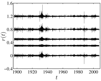
Fig. 3 compares the original return series with four surrogate time series generated from a normal distribution, a Laplace distribution, a Weibull distribution with , and a Student distribution with , respectively. We can see that all the surrogate series exhibit similar clustering phenomenon as the original returns. In other words, the volatility (absolute value) of the surrogate data has long-term correlation, which is still true for all the cases. This intriguing feature is very important since it is absent in the surrogate data according to the phase randomization algorithm. In addition, the two surrogate series with fat tails share more similarity with the original returns than those from the normal and Laplace distributions. Certainly, a close scrutiny of the time series will unveil differences in their finer structure.
For the case of Weibull distributions, we investigate 11 values of the exponent , varying from 0.45 to 0.95 with a spacing step of 0.05. For smaller values, we find that the multifractal spectra are not stable due to the poor statistics caused by extreme jumps in the time series. For each , we generate 100 surrogate time series and the average multifractal spectrum is determined. The multifractal spectra for , 0.55, 0.65, 0.75, 0.85 and 0.95 are illustrated in fig. 4(a). It is evident that time series with heavier tails (or small ) exhibits stronger multifractality. This quantitative dependence of the average singularity width as a function of the exponent is depicted in fig. 4(b).
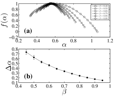
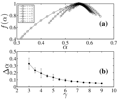
For the case of Student distributions, we investigate 13 values for the tail exponent , varying from 3 to 9 with a spacing step of 0.5. We choose the minimal value of since the returns at the transaction level are well modeled by Student’s t distribution with [63], which is the well-known inverse cubic law [64], and the tail exponent increases with the time scale [1]. For each , we generate 100 surrogate time series and the average multifractal spectrum is determined. Figure 5(a) illustrates the multifractal spectra for , 4, 5, 6, 7, 8 and 9. Again, it is evident that time series with heavier tails (or small ) exhibits stronger multifractality. Comparing with fig. 4(a), we find that the right parts of the curves for the Student’s t distributions are closer to each other, which means that the small values characterized by negative ’s are more irregular. The quantitative dependence of the average singularity width as a function of the exponent is shown in fig. 5(b).
4 Hidden nonlinear structure
In the above analysis, we have investigated the impact of temporal correlation and probability distribution on the multifractal nature. More rigorously speaking, the shuffling approach is very aggressive, which not only removes linear correlations but also eliminates any hidden structure in the original return series. It is thus interesting to assess the impact of hidden structure. This can be done with the help of surrogate time series which has the same distribution and linear temporal correlation as the original data. We find that the DFA scaling exponent of the DJIA returns is . Although the DFA scaling exponent is very close to 0.5 for uncorrelated time series, it may still contain some nontrivial information about the linear correlation in the original series. It is worth noting that this method will be more interesting for other financial time series whose DFA scaling exponent is significantly larger than 0.5 and thus have long memory.
The algorithm for the generating of surrogate data is based on a simple iteration scheme called iterated amplitude-adjusted Fourier transform (IAAFT) [65], which is an improved version of the phase randomization algorithm [60]. The return data are sorted resulting in a new sequence , and we obtain the squared amplitudes of the Fourier transform of , denoted as . The initial sequence of the iteration is a random shuffle of . In the -th iteration, the squared amplitudes of the Fourier transform of are obtained and replaced by , which are transformed back, and then the resulting series are replaced by but keeping the rank order. We generate 100 surrogate time series and perform the iteration 20 times for each surrogate series.
Fig. 6 plots the averaged multifractal spectrum of the surrogate series and the curve of the original return series as well. The singularity width is for the surrogate data, which is close to for the original data. For the right part where , the curve for surrogate data is embraced by that for the original data. For the left part where , the two curves almost overlap with the error bar for a large part. We also observe that the surrogate data have negative dimensions, which implies that the surrogate data contain more randomness in large values of local detrended fluctuations [58, 59].
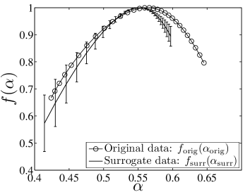
It is also interesting to compare the curve for the surrogate data in fig. 6 and for the shuffled data in fig. 1. We find that these two curves and have the same shape with a horizontal shift. We have approximately that
| (7) |
where . Note that the value of is close to the difference of the two DFA scaling exponents, , where and . Since , this relation can be understood as a first-order approximation in the sense that . The relation (7) means that the difference between the multifractal spectra of the surrogate and shuffled data is caused by the weak temporal correlation remained in the surrogate data. In general, the linear correlation in the time series does not influence the shape of the singularity spectrum (and thus its width) but rather has a shift effect.
To further quantify the presence of hidden nonlinear features in the return time series and their effect on the multifractal spectrum, some remarks are in order based on the magnitude and sign decomposition method [66, 67]. The daily DJIA return series can be decomposed into a magnitude (or volatility) series and a sign series. We find that the DFA scaling exponent of the magnitude series is 0.87, confirming the well-known stylized fact that stock market volatility has strong long memory. In contrast, the magnitude series of the shuffled and the IAAFT surrogates are found to be uncorrelated. These facts confirm the presence of nonlinearity in the return time series. It is well established that the phase-randomized surrogates of heartbeat series have a vanishing width of singularity [68, 69], which is due to the fact that the heartbeat time series do not have fat tails, but decay exponentially [70].
5 Conclusions
In summary, we have systematically studied the components of empirical multifractality in financial returns based on shuffled and surrogate data, taking the daily data of DJIA for more than one hundred years as an example. We found that the distribution, the linear correlation, and the nonlinear structure have influence on the singularity spectrum. When the degree of multifractality is characterized by the singularity width , we found that the temporal structure (linear correlation and nonlinearity) has minor impact while the fat-tailed distribution plays a major role, which is a confirmation of the earlier results.
Acknowledgements.
I am grateful to Gao-Feng Gu, Zhi-Qiang Jiang and Guo-Hua Mu for fruitful discussions. This work was partly supported by Shanghai Educational Development Foundation (2008SG29) and the Program for New Century Excellent Talents in University (NCET-07-0288).References
- [1] \NameGhashghaie S., Breymann W., Peinke J., Talkner P. Dodge Y. \REVIEWNature 3811996767.
- [2] \NameMantegna R. N. Stanley H. E. \REVIEWNature 3831996587.
- [3] \NameMandelbrot B. B. \REVIEWSci. Am. 298199970.
- [4] \NameEisler Z., Kertész J., Yook S.-H. Barabási A.-L. \REVIEWEurophys. Lett. 692005664.
- [5] \NameEisler Z. Kertész J. \REVIEWEPL 77200728001.
- [6] \NameJiang Z.-Q., Guo L. Zhou W.-X. \REVIEWEur. Phys. J. B 572007347.
- [7] \NameVandewalle N. Ausloos M. \REVIEWEur. Phys. J. B 41998257.
- [8] \NameIvanova K. Ausloos M. \REVIEWEur. Phys. J. B 81999665.
- [9] \NameSchmitt F., Schertzer D. Lovejoy S. \REVIEWAppl. Stoch. Models Data Anal. 15199929.
- [10] \NameSchmitt F., Schertzer D. Lovejoy S. \REVIEWInt. J. Theoret. Appl. Financ. 32000361.
- [11] \NameCalvet L. Fisher A. \REVIEWRev. Econ. Stat. 842002381.
- [12] \NameAusloos M. Ivanova K. \REVIEWComput. Phys. Commun. 1472002582.
- [13] \NameGórski A. Z., Drożdż S. Speth J. \REVIEWPhysica A 3162002496.
- [14] \NameAlvarez-Ramirez J., Cisneros M., Ibarra-Valdez C. Soriano A. \REVIEWPhysica A 3132002651.
- [15] \NameBalcilar M. \REVIEWEmerging Markets Financ. Trade 3920035.
- [16] \NameLee K. E. Lee J. W. \REVIEWJ. Korean Phys. Soc. 462005726.
- [17] \NameLee J. W., Lee K. E. Rikvold P. A. \REVIEWPhysica A 3642006355.
- [18] \NameJiang Z.-Q. Zhou W.-X. \REVIEWPhysica A 3812007343.
- [19] \NameKantelhardt J. W., Zschiegner S. A., Koscielny-Bunde E., Havlin S., Bunde A. Stanley H. E. \REVIEWPhysica A 316200287.
- [20] \NameMatia K., Ashkenazy Y. Stanley H. E. \REVIEWEurophys. Lett. 612003422.
- [21] \NameKwapień J., Oświȩcimka P. Drożdż S. \REVIEWPhysica A 3502005466.
- [22] \NameLee K. E. Lee J. W. \REVIEWJ. Korean Phys. Soc. 472005185.
- [23] \NameOświȩcimka P., Kwapień J. Drożdż S. \REVIEWPhysica A 3472005626.
- [24] \NameJiang J., Ma K. Cai X. \REVIEWPhysica A 3782007399.
- [25] \NameLee K. E. Lee J. W. \REVIEWPhysica A 383200765.
- [26] \NameLim G., Kim S., Lee H., Kim K. Lee D.-I. \REVIEWPhysica A 3862007259.
- [27] \NameSu Z.-Y., Wang Y.-T. Huang H.-Y. \REVIEWJ. Korean Phys. Soc. 5420091395.
- [28] \NameSun X., Chen H.-P., Wu Z.-Q. Yuan Y.-Z. \REVIEWPhysica A 2912001553.
- [29] \NameSun X., Chen H.-P., Yuan Y.-Z. Wu Z.-Q. \REVIEWPhysica A 3012001473.
- [30] \NameHo D.-S., Lee C.-K., Wang C.-C. Chuang M. \REVIEWPhysica A 3322004448.
- [31] \NameWei Y. Huang D.-S. \REVIEWPhysica A 3552005497.
- [32] \NameGu G.-F., Chen W. Zhou W.-X. \REVIEWEur. Phys. J. B 57200781.
- [33] \NameDu G.-X. Ning X.-X. \REVIEWPhysica A 3872008261.
- [34] \NameZhuang X.-T. Yuan Y. \REVIEWPhysica A 3872008511.
- [35] \NameWei Y. Wang P. \REVIEWPhysica A 38720081585.
- [36] \NameZhou W.-X. \REVIEWJ. Manag. Sci. China (in Chinese) 132010in press.
- [37] \NameJiang Z.-Q. Zhou W.-X. \REVIEWPhysica A 38720083605.
- [38] \NameSu Z.-Y. Wang Y.-T. \REVIEWJ. Korean Phys. Soc. 5420091385.
- [39] \NameStruzik Z. R. Siebes A. P. J. M. \REVIEWPhysica A 3092002388.
- [40] \NameTuriel A. Pérez-Vicente C. J. \REVIEWPhysica A 3222003629.
- [41] \NameTuriel A. Pérez-Vicente C. J. \REVIEWPhysica A 3552005475.
- [42] \NameOświȩcimka P., Kwapień J., Drożdż S. Rak R. \REVIEWActa Phys. Pol. B 3620052447.
- [43] \NameZunino L., Tabak B. M., Figliola A., Pérez D. G., Garavaglia M. Rosso O. A. \REVIEWPhysica A 38720086558.
- [44] \NameBouchaud J.-P., Potters M. Meyer M. \REVIEWEur. Phys. J. B 132000595.
- [45] \NameSaichev A. Sornette D. \REVIEWPhys. Rev. E 742006011111.
- [46] \NameLux T. \REVIEWInt. J. Modern Phys. C 152004481.
- [47] \NameKumar S. Deo N. \REVIEWPhysica A 38820091593.
- [48] \Namede Souza J. Queirós S. M. D. \REVIEWChaos, Solitons & Fractals 4220092512.
- [49] \NameDrożdż S., Kwapień J., Oświecimka P. Speth J. \BookQuantitative features of multifractal subtleties in time series arXiv: 0907.2866 (2009).
- [50] \NameNakao H. \REVIEWPhys. Lett. A 2662000282.
- [51] \Namevon Hardenberg J., Thieberger R. Provenzale A. \REVIEWPhys. Lett. A 2692000303.
- [52] \NameOh G., Eom C., Havlin S., Jung W.-S., Wang F.-Z., Stanley H. E. Kim S. \REVIEWPhys. Rev. E XXX2010XXX.
- [53] \NameNorouzzadeh P. Rahmani B. \REVIEWPhysica A 3672006328.
- [54] \NameHu K., Ivanov P. C., Chen Z., Carpena P. Stanley H. E. \REVIEWPhys. Rev. E 642001011114.
- [55] \NameChen Z., Ivanov P. C., Hu K. Stanley H. E. \REVIEWPhys. Rev. E 652002041107.
- [56] \NameChen Z., Hu K., Carpena P., Bernaola-Galvan P., Stanley H. E. Ivanov P. C. \REVIEWPhys. Rev. E 712005011104.
- [57] \NameHalsey T. C., Jensen M. H., Kadanoff L. P., Procaccia I. Shraiman B. I. \REVIEWPhys. Rev. A 3319861141.
- [58] \NameMandelbrot B. B. \REVIEWPhysica A 1631990306.
- [59] \NameMandelbrot B. B. \REVIEWProc. R. Soc. Lond. A 434199179.
- [60] \NameTheiler J., Eubank S., Longtin A., Galdrikian B. Farmer J. D. \REVIEWPhysica D 58199277.
- [61] \NameBogachev M. I., Eichner J. F. Bunde A. \REVIEWPhys. Rev. Lett. 992007240601.
- [62] \NameZhou W.-X. \REVIEWPhys. Rev. E 772008066211.
- [63] \NameGu G.-F., Chen W. Zhou W.-X. \REVIEWPhysica A 3872008495.
- [64] \NameGopikrishnan P., Meyer M., Amaral L. A. N. Stanley H. E. \REVIEWEur. Phys. J. B 31998139.
- [65] \NameSchreiber T. Schmitz A. \REVIEWPhys. Rev. Lett. 771996635.
- [66] \NameAshkenazy Y., Ivanov P. C., Havlin S., Peng C.-K., Goldberger A. L. Stanley H. E. \REVIEWPhys. Rev. Lett. 8620011900.
- [67] \NameAshkenazy Y., Havlin S., Ivanov P. C., Peng C.-K., Schulte-Frohlinde V. Stanley H. E. \REVIEWPhysica A 323200319.
- [68] \NameIvanov P. C., Amaral L. A. N., Goldberger A. L., Havlin S., Rosenblum M. G., Struzik Z. R. Stanley H. E. \REVIEWNature 3991999461.
- [69] \NameIvanov P. C., Amaral L. A. N., Goldberger A. L., Havlin S., Rosenblum M. G., Stanley H. E. Struzik Z. R. \REVIEWChaos 112001641.
- [70] \NameIvanov P. C., Rosenblum M. G., Peng C.-K., Mietus J. E., Havlin S., Stanley H. E. Goldberger A. L. \REVIEWPhysica A 2491998587.