AIPbodytext
0pt0pt0pt plus 1fil
0pt
\DeclareParagraphLayoutXFMtitle
18pt19pt
0pt0pt
0pt
\SetInternalRegister2000
\SetInternalRegister20000
\DeclareParagraphLayoutXFMauthors
14pt15pt
0pt0pt
0pt
\SetInternalRegister2000
\SetInternalRegister20000
\DeclareParagraphLayoutXFMaddress
12pt14pt
0ptplus 1fil
plus 1fil0pt
0pt
\SetInternalRegister2000
\SetInternalRegister20000
\DeclareParagraphLayoutXFMabstracttext
11pt14pt
1pc0pt0pt0pt plus 1fil
0pt
\DeclareParagraphLayoutXFMclassificationtext
10pt13pt
0pt0pt plus 1fil
0pt
\DeclareParagraphLayoutAliasXFMkeywordstextXFMclassificationtext
\AIP@cmdnotsupported
Network harness: bundles of routes in public transport networks
Abstract
Public transport routes sharing the same grid of streets and tracks are often found to proceed in parallel along shorter or longer sequences of stations. Similar phenomena are observed in other networks built with space consuming links such as cables, vessels, pipes, neurons, etc. In the case of public transport networks (PTNs) this behavior may be easily worked out on the basis of sequences of stations serviced by each route. To quantify this behavior we use the recently introduced notion of network harness. It is described by the harness distribution : the number of sequences of consecutive stations that are serviced by parallel routes. For certain PTNs that we have analyzed we observe that the harness distribution may be described by power laws. These power laws observed indicate a certain level of organization and planning which may be driven by the need to minimize the costs of infrastructure and secondly by the fact that points of interest tend to be clustered in certain locations of a city. This effect may be seen as a result of the strong interdependence of the evolutions of both the city and its PTN.
To further investigate the significance of the empirical results we have studied one- and two-dimensional models of randomly placed routes modeled by different types of walks. While in one dimension an analytic treatment was successful, the two dimensional case was studied by simulations showing that the empirical results for real PTNs deviate significantly from those expected for randomly placed routes.
Keywords:
\AIP@errorMissing declaration Specify a list of keywords <Missing keywords>Keywords:
complex networks, harness effect, public transport:
\AIP@errorMissing declarationSpecify PACS number(s) choosing from http://www.aip.org/pacs/index.html <Missing classification>:
02.50.-r, 07.05.Rm, 89.75.Hc1 Introduction
A variety of different phenomena have in recent years been analyzed in the context of complex network theory [1, 2]. Usually, the focus is on the network topology while the study of specific features as e.g. the network load or real-space correlations is mostly left aside.222Paper presented at the Conference “Statistical Physics: Modern Trends and Applications” (23-25 June 2009, Lviv, Ukaine) dedicated to the 100th anniversary of Mykola Bogolyubov (1909-1992).
Analyzing statistical properties of public transport networks (PTNs) [3, 4, 5] a so-called harness effect which results from such spatial correlations has recently been proposed [5, 6]. The latter may be observed for networks on which a set of walks or paths is defined. Indeed, public transport routes sharing the same grid of streets and tracks define such a set of walks on this grid. Often these are found to proceed in parallel along shorter or longer sequences of stations. Similar phenomena are observed in other networks built with space consuming links such as cables [7], vessels [8], pipes [9], neurons [10], etc. In the case of PTNs, a quantitative description of sequences of stations that are served by several routes may be performed in the form of the harness distribution : the number of maximal found on the network sequences of consecutive stations that are serviced by parallel routes. In a recent empirical analysis of the harness effect on PTNs of 14 major cities in the world [5, 6] it was found that for certain cities the behavior of the function is described by power laws. These observed power laws indicate a certain level of organization and planning which may be driven by the need to minimize the costs of infrastructure and secondly by the fact that points of interest tend to be clustered in certain locations of a city.
In the present paper, to further investigate the significance of the empirical results we have studied one- and two-dimensional models of randomly placed routes modeled by different types of walks. The setup of the paper is the following. First we recall some results of the empirical analysis. We then proceed solving a simple 1d model of a growing non-correlated network that allows an analytical treatment. Finally we analyze different types of growing networks on the 2d square lattice and perform numerical simulations and measure the resulting harness effect as function of the model parameters. Conclusions are given in the last section.
2 Results of an empirical analysis
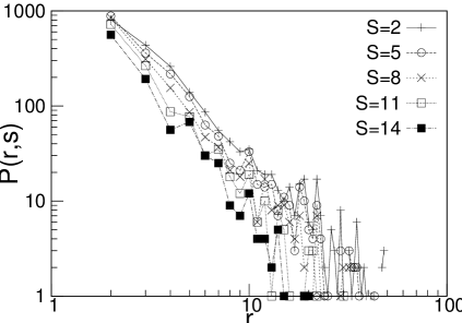
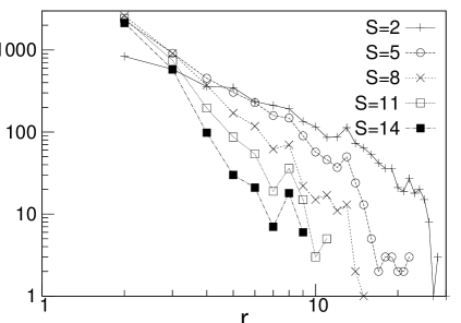
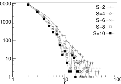
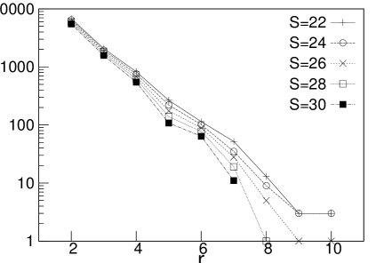
In a previous study we have analyzed the PTNs of 14 major cities that have different geographical, historical and cultural background [5, 6]. For some of these we observed non-vanishing harness distributions even for long sequences and high numbers of routes . This is what we call a "strong"harness effect (examples are Sao Paolo, Hong Kong, Istanbul, Los Angeles, Rome, Sydney, Taipei, Moscow, London; some are shown in Fig. 1). For other PTNs the maximal values of and with were found to be smaller than 10 (Berlin, Paris, Dallas, Duesseldorf, Hamburg) - this we call a "weak"harness effect (Fig. 2). It is important to note that the division into these two classes does not correlate with either the average number of routes in the PTN or their average length .
 |
 |
| (a) | (b) |
 |
 |
| (c) | (d) |
Another result is that similar to the node-degree distributions [5, 6] we observe that the harness distribution for some of the cities (Sao Paolo, Hong-Kong, Istanbul, Los Angeles, Rome, Sydney) may be described by a power law:
| (1) |
whereas the PTNs of other cities (Taipei, Moscow, London, Hamburg) are better described by an exponential decay:
| (2) |
We illustrate this behaviour in Figs. 1a,b showing the harness distribution for Istanbul and for Taipei. In some cases (e.g. for Rome and Los Angeles) there is a crossover between regimes (1) and (2) at larger as shown this for the PTN of Los Angeles (Fig.1c). Here, one can see that for small values of the results are better described by a power law (1). With increasing a tendency to an exponential decay (2) appears (Fig. 1d). This is less obvious for other cities analyzed, however in all cases the harness distribution as function of decays faster for longer sequence lengths and while also attaining a more pronounced curvature.
Note that in Fig. 1 we plot -cumulative distributions where a sequence with maximal length will be counted once as a sequence of length and twice as a sequence of length etc:
| (3) |
It may be surprising that these curves e.g. for Taipei (Fig. 1b) intersect for low values of . We will discuss this effect below.
For PTNs for which the harness distribution follows a power law (1) the corresponding exponents are found in the range of . For those distributions with an exponential decay the scale (see eq.(2) varies in a range . The power laws observed for the behavior of indicate a certain level of organization and planning which may be driven by the need to minimize the costs of infrastructure and secondly by the fact that points of interest tend to be clustered in certain locations of a city. Note that this effect may be seen as a result of the strong interdependence of the evolutions of both the city and its PTN. We want to emphasize that the harness effect is a feature of the network given in terms of its routes but it is invisible in any of the complex network representations of public transport networks presented so far, such as L-space [3], P-space [11] or B-space [5, 12]. It is possible, that the notion of harness may be useful also for the description of other networks with similar properties. On the one hand, the harness distribution is closely related to distributions of flow and load on the network. On the other hand, in the situation of space-consuming links (such as tracks, cables, neurons, pipes, vessels) the information about the harness behavior may be important with respect to the spatial optimization of networks. A generalization may be readily formulated to account for real-world networks in which links (such as cables) are organized in parallel over a certain spatial distance. While for the PTN this distance is simply measured by the length of a sequence of stations, a more general measure would be the length of the contour along which these links proceed in parallel.
For the cities observed no correlation appears to occur between the harness distribution behavior and other well-known network characteristics that were analyzed, as for example the node-degree distribution of PTNs [5].
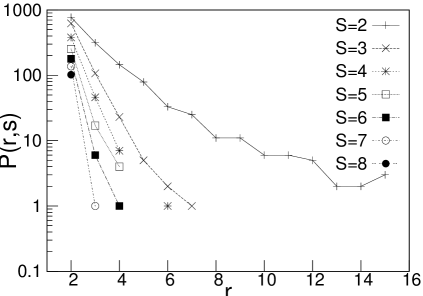
However, the extent to which harness properties are expressed may obviously play a role for the attack vulnerability of a PTN. Interestingly, our previous investigations have shown that the Paris PTN is most resilient to any type of random or directed attacks (in terms of percolation concepts) among all analyzed PTNs [13]. At the same time it exhibits the "weakest"behavior with respect to the harness effect (Fig. 2). One may expect such a result: routes that do not share the same streets are more resilient. However, for other cities no apparent correlation between harness effect behavior and their vulnerability has been found so far.
As noted above the interesting question to answer is: are there any structural evolution purposes behind this effect, or can it be found just as well within simple random scenarios.
3 Analytic results and modeling in 1d
Let us first investigate a network model with routes placed randomly in one dimensional
space. Although being very simple this model can mimic a harness
effect and as we will see below, it allows an analytical solution. The
model is formulated in the following way:

The left terminals of routes of length are placed at random on a line with N sites, with periodic boundary conditions. E.g. in Fig.3 we show two routes of length with left terminals at and . We define the route density as routes per site.
The distribution of left-terminals on a given site, e.g. site will be : the probability that routes have their left-terminal on site
| (4) |
where the first term counts the number of ways to select of routes, the second term is the probability that the left terminals lie on site and the third term is the probability that no left terminal of an unselected route lies on site . In other words, by definition is a binomial distribution. For , but fixed this distribution has the limiting behavior of a Poisson distribution:
| (5) |
Let us now calculate the probability that there is a sequence of maximal length and maximal width of routes in parallel between sites and . This implies that at least one of the routes starts at and at least one of the routes ends at . The latter route then starts at (Fig. 3). The other routes may start anywhere in between . We denote the number of routes starting at as , those starting at as .
In the limit and we may consider , , … , as independent probabilities (this is not true for small systems, however, as we see later the correlation between these probabilities is negligible for the cases studied here. The overall probability to find a sequence of length and width starting at is then the sum over all combinations leading to the result:
| (6) |
where denotes a sum over with .
Now, without the conditions and this sum can be derived from:
| (7) |
The sum with these conditions however can be written as:
| (8) |
Thus:
| (9) |
With this formula we count sequences that start at . To receive the overall probability this is to be multiplied by .
| (10) |
Simple arithmetic allows us to calculate the -cumulative distributions , see eq. (3).
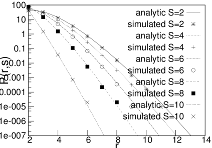
As mentioned above, the probabilities we use are appropriate for infinite systems. To test their validity for finite cases we performed some simple simulations.
 |
 |
| (a) | (b) |
 |
 |
| (c) | (d) |
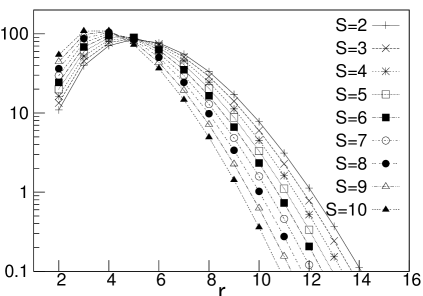
It turns out that the average results fit this formula with very good accuracy even for small , for example and of course for any larger values of (Fig. 4a). For a large range of parameters , , the behavior of looks similar to what is shown in Fig. 4b. For high overall density we observe that curves for different intersect at small as for some real-world PTNs. In one dimension, this effect has the following explanation: when the space is overcrowded one will in general find more than two routes to overlap for small sequences of stations.
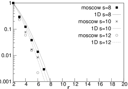
This model has three parameters: the number of routes , the route length and the number of sites . As is obvious from eq. (10) the harness distribution for all and is close to a Poisson decay (5) for any set of parameters. Therefore PTNs with an exponential behavior of the harness distribution may be compared with the results of the one-dimensional approach. As an example we compare the normalized harness distribution for Moscow and the one-dimensional set of lines (Fig. 4c,d), where the number of routes and the route length were chosen to match those of the Moscow PTN ( set to the average route length).
However, the quantitative results for all observed PTNs are several orders of magnitude higher than the result obtained with (9) in one dimension for the same and (for any ). Furthermore, PTNs that show a power law behavior (1) are even qualitatively different from the random 1D approach. Another difference is that the harness distribution curves for different are very similar in shape and both slope and curvature vary much less than for the PTN harness distributions.
In the following we test a two-dimensional model with the simple simulations.
4 Simple 2d modeling
It is obvious that simply throwing at random lines parallel to the axis’ of a 2d square lattice with periodic boundary conditions will lead to the original 1d problem: If the lattice has sites one would get independent one-dimensional systems. However, it is not a priory clear what results one will find for more general sets of walks on a 2d square lattice.
 |
 |
| (a) | (b) |
 |
(c) |
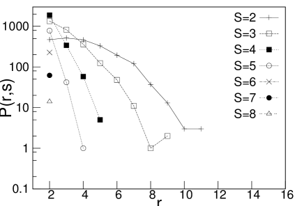
To work this out, we implemented the following simulations. We work on a 2d square lattice with periodic boundary conditions. On this lattice we chose a set of walks each of length (number of steps plus 1). The routes are built either as random walks (RW), non-reversal random walks (NRRW) that cannot reverse the previous step, or self-avoiding random walks (SAW), that may not intersect themselves.
These models have three parameters: the number of routes , the route length and the lattice size . We choose the first two parameters to match those of different real PTNs.
Postponing a more detailed analysis to a separate publication we here summarize some of the main features of the harness distribution of these models. Besides the finding that the harness effect is "weak some similarity between the the harness effects seen in the three models is observed (Fig 5a,b,c). Curvature and slope evolve in a similar way. Also intersections between the curves for different are found to occur at lower values of in all cases. Differences are that the RW-generated networks demonstrate a "weaker"harness effect, while NRRW- and SAW-generated networks result in harness distributions of similar order of magnitude.
It turns out that for fixed and , increasing the lattice size , the harness distributions , for all fixed and show non-monotonous behavior (Fig. 6). As function of it first increases, and then after reaching a maximum it starts to decrease. Comparing with the empirical values found for real PTNs we observe, that for some PTNs the empirical values even for small and are significantly larger than the maximum that could be obtained with RW. For NRRW or SAW the empirical values are within the observed range, however only for a small interval of .
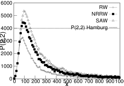
This proves numerically the not surprising observation, that with any of the proposed random or quasi-random walks only a very "weak"harness effect may be obtained. In turn, this strongly indicates that for most of the observed cities the harness effect must have a structural background, that is not to be modeled by any of the random approaches taken here.
Let us therefore analyze the harness effect for a model that intrinsically takes correlations into account using some ideas of non-equilibrium network evolution. [5].
5 An evolutionary model in 2d
From previous studies of PTNs [4, 5] the following facts are relevant for our further discussion of PTN network evolution. The final network often displays features (a power law degree distribution) that are compatible with a preferential attachment scenario [1]. Furthermore, the fractal dimension of public transport routes appears to match that of 2d self-avoiding walks [5]. This leads to the following model.
Given a 2d square lattice with side and periodic boundary conditions, routes each of length will be created in the following way. A first route is built as self-avoiding walk. Let be the number of visits to lattice site . The subsequent routes are constructed as SAWs with the following preferential attachment rules:
a) choose a terminal station at with probability
| (11) |
a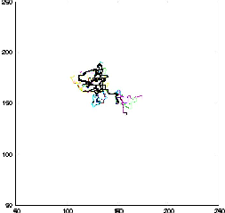 b
b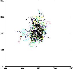 c
c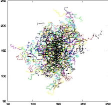
a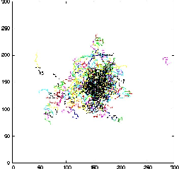 b
b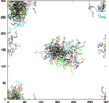 c
c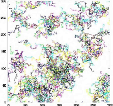
b) choose any subsequent station of the route with probability
| (12) |
c) If route intersects itself, discard it and return to step a).
Repeat steps a)-c) until routes are created.
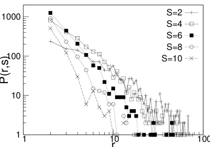
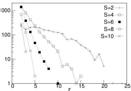
We call this model the model of mutually interacting self-avoiding walks (MI SAW). It implements a preferential attachment scenario for networks that are built from chains (routes in our case). On the figures presented (Fig. 7-8) one can see how the parameters and influence the distribution of the routes on the lattice. Parameter controls the number of disconnected clusters, while parameter is related to the spread of each cluster. If both parameters equal zero, all routes are restricted to the sites occupied by the first route.
 |
 |
| (a) | (b) |
 |
 |
| (c) | (d) |
To present the obtained results we show the harness distribution for different values for the model parameters and (Fig. 9). It turns out that for choosing different values we may either find a behavior that corresponds to a power law distribution (Fig. 9a,b) or a behavior that corresponds to an exponential decay (Fig. 9c,d).
Also other features of real-world PTNs may be reproduced. With increasing the sequence length the harness distribution as a function of the number of routes attains a stronger curvature and a steeper slope. Thus, with increasing sequence length there is a cross-over from the power law regime (1) to an exponential regime (2).
In the same way as observed for real-world PTNs in the 1d approach and also for simple 2d models on the square lattice the -cumulative harness distributions as function of the number of routes intersect at low values of . In one dimension we observed this behaviour because of an overcrowding effect, see above. This also occurs to some extent in the 2d case, however, on the 2d lattice there is an additional combinatorial effect that leads to this result: the number of different possible configurations of sequences with length is smaller than the corresponding number of different possible configurations with length . To summarize one can say that the MI SAW model reproduces a large amount of the empirically observed behavior of harness distributions of PTNs.
6 Conclusions
Harness phenomena may be observed in different networks built with space consuming links such as cables, vessels, pipes, neurons, etc. The present analysis may possibly be applied also to such types of networks. In the particular case of the PTNs that we have analyzed we observe that in some cases the harness distribution may be described by power laws. These observed power laws indicate a certain level of organization and planning which may be driven by the need to minimize the costs of infrastructure and secondly by the fact that points of interest tend to be clustered in certain locations of a city. This effect may be seen as a result of the strong interdependence of the evolutions of both the city and its PTN.
To further investigate the significance of the empirical results we have studied one- and two-dimensional models of randomly placed routes modeled by different types of walks. While in one dimension an analytic treatment was successful, the two dimensional case was studied by extensive simulations.
Our main results are the following:
-
•
A one dimensional model for harness distributions was solved analytically.
-
•
Exponentially decaying harness distributions may be reproduced by the 1d approach.
-
•
Simple random placement of RW, SAW or NRRW on a two dimensional square lattice result in weak harness distributions; in the RW case much weaker than for real PTNs.
-
•
The -cummulative distributions for different intersect at low values of for all models due to combinatorial reasons.
-
•
A model of mutually interacting SAWs reproduces many of the empirically observed features of harness distributions.
REFERENCES
-
(1)
1. R. Albert, and A.-L. Barabási, Statistical Mechanics of
Complex Networks, Rev. Mod. Phys., 74, pp. 47-97, (2002).
-
(2)
2. S. N. Dorogovtsev, and J. F. F. Mendes. Evolution of
Networks, Oxford University Press, Oxford, (2003).
-
(3)
3. V. Latora, and M. Marchiori, Is the Boston subway a
small-world network, Physica A, 314, pp. 109-113 (2002)
-
(4)
4. J. Sienkiewicz, and J. A. Holyst, Statisctical analysis of
22 public transport networks in Poland, Phys. Rev. E, 72,
046127, (2005).
-
(5)
5. C. von Ferber, T. Holovatch, Yu. Holovatch, and V. Palchykov,
Network harness: Metropolis public transport, Physica A,
380, pp. 585-591 (2007); Public transport networks:
empirical analysis and modeling, Eur. Phys. J. B, 68, 2,
pp. 261-275, (2009).
-
(6)
6. C. von Ferber, Yu. Holovatch, and V. Palchykov, Scaling in
Public Transport Networks, Condens. Matter Phys., 8, No.
1(41), pp. 225-234, (2005).
-
(7)
7. M. R. Cutkosky, A. B. Conru, and S-H. Lee, An agent-based
approach to concurrent cable harness design, AIEDAM, 8,
No. 1, (1994).
-
(8)
8. P. Carmeliet, and M. Tessier-Lavigne, Common mechanisms of
nerve and blood vessel wiring, Nature, 436, pp. 193-200,
(2005).
-
(9)
9. N. Hwang, and R. Houghtalen, Fundamentals of hydraulic
Engineering Systems, Prentice Hall, Upper Saddle River, NJ, (1996).
-
(10)
10. J. G. White, E. Southgate, J. N. Thompson, and S. Brenner,
The structure of the nervous system of the nematode C.
Elegans, Philos. Trans. Roy. Soc. London, 314, pp. 1–340,
(1986).
-
(11)
11. P. Sen, S. Dasgupta, A. Chatterjee, P. A. Sreeram, G. Mukherjee,
and S. S. Manna, Small-world properties of the Indian railway
network, Phys. Rev. E, 67, 036106, (2003).
-
(12)
12. J.-L. Guillaume, and M. Latapy, Bipartite graphs as models
of complex networks, Physica A, 317, pp. 795-813 (2006);
- (13) 13. B. Berche, C. von Ferber, T. Holovatch, and Yu. Holovatch, Resilience of public transport networks against attacks, arXiv:0905.1638v1; Eur. Phys. J. B, submitted, (2009).
- (14)