Nonlocal transport through multiterminal diffusive superconducting nanostructures

Abstract

Motivated by recent experiments on nonlocal transport through multiterminal superconducting hybrid structures, we present self-consistent calculations based on quasiclassical Green’s functions for the order parameter, currents and voltages in a system consisting of a diffusive superconductor connected to two normal and one superconducting electrodes. We investigate non-equilibrium effects for different biasing conditions corresponding to measurements of the nonlocal conductance and of the nonlocal resistance. It is shown that while the nonlocal conductance does not change its sign, this change might be observed in a nonlocal resistance measurement for certain parameter range. The change of sign of the nonlocal signal takes places at a voltage of the order of the self-consistent gap of the superconducting region. We show that this is not related to the nonlocal Andreev processes but rather to non-equilibrium effects. We finally discuss the case of four terminal measurements and demonstrate that a change of sign in the nonlocal resistance appears when the current injected into the superconductor exceeds a critical value. The connection to the existing experiments is discussed.

I Introduction

The possibility to create and control entangled electron pairs from a superconductor has renewed the interest in transport through superconductor-normal metal hybrid structures beckmann ; delft ; chan ; beckmann2 ; basel . The basic idea is to exploit the long-range coherence of the Andreev reflectionandreev , in order to couple two spatially separated normal electrodes connected to a superconducting region within a distance of the order of the superconducting coherence length $\xi_{S}$. An Andreev processes that takes place at two different interfaces is called a ”crossed”’ Andreev reflection (CAR). As suggested in Ref. byers spatial correlations can be probed by nonlocal transport experiments. A typical setup for detection of CAR processes consists of a grounded superconducting region (S) connected to normal electrodes (N). The information on such processes would be encoded, for instance, in the voltage which is measured in one of the S/N interfaces when a current is injected through the other one. Besides CAR processes, individual electrons can also tunnel across the superconductor. This normal tunneling has been called “elastic cotunneling” (EC). CAR and EC contributions to the non-local conductance have opposite signs, and in the lowest order of tunneling cancel each otherfalci . For higher orders in the tunneling the EC dominates over CAR regis and the nonlocal signal becomes finite. Surprisingly a change of sign in the nonlocal resistance and conductance was reported as a function of the local voltage for a NSN layered structuredelft and a FSF multiterminal structurebeckmann2 (F denotes a ferromagnetic metal). According to Ref.delft by low (high) voltages EC (CAR) processes dominate the nonlocal transport. Similar behavior was observed in Ref.beckmann2 for samples with high S/F barrier resistance. The latter experiment also showed dominance of CAR processes at low voltages for samples with higher interface transparency. These experimental results have lead to several theoretical works regis ; kalenkov ; morten ; golubov ; golubev ; natphys ; zaikin09 ; prb09 , which attempt to find a microscopic description for those observations. However, up to now theories based on non-interacting models could not explain the change of sign of the non-local conductance kalenkov ; morten ; golubov ; golubev . For a layered NSN structure, as the one of Ref. delft , the change of sign of the non-local conductance has been explained by taking into account interaction of the conducting electrons with their electromagnetic environmentnatphys . The later description is valid in the tunneling limit, thus the observation of negative non-local conductances in the case of good interface transparencies remains without microscopic explanation yet.

In principle, a description of the non-local transport in terms of CAR and EC is only valid in the tunneling limit. In this case the system is in a quasi-equilibrium state, i.e. the current (or the corresponding bias voltage) is much smaller than its critical value and the distribution function of quasiparticles is the equilibrium one. This assumption has been made in most of the theoretical works mentioned above. In particular the superconducting gap was assumed to have the bulk value, i.e. the superconducting order parameter was not affected by the possible deviation of the distribution function from its equilibrium value. In some experiments though, this is not the case. For example in Refs. chan ; basel ; beckmann the transparencies of the S/N interfaces are not necessarily low, and in Ref. chan the current injected into the S region reached its critical value. Thus, for a proper description of these experiments one needs to go beyond the quasi-equilibrium approach. A first attempt was done in Refsprb09 ; zaikin09 . It was shown that non-equilibrium effects may play a crucial role on the non-local transport properties. In particular, in Ref. prb09 self-consistent calculations based on a two dimensional tight binding model were implemented. It was shown that far from the quasiequilibrium regime the nonlocal transport cannot longer be described in simple terms of EC and CAR processes. For some set of parameters, a change of sign in the non-local resistance was obtained. This change of sign is not related to the predominance of CAR but rather to the possibility of having a negative local conductance at the interface where the current is injected. In Ref.zaikin09 a non-monotonic behavior of the non-local resistance as a function of the temperature was obtained, which resembles the observations of Ref. chan . However, the non-local resistance as a function of the injected current or bias voltage was not investigated in that work.

In the above mentioned theoretical works, one computes the non-local conductance in a three terminal device. In other words, one assumes that one of the normal terminals is biased to a voltage $V_{L}$, while the second normal terminal is grounded. In this way one determines the current $I_{R}$ flowing into the latter terminal and computes the non-local conductance $G_{nl}=dI_{R}/dV_{L}$. Experimentally, however, it is simpler to fix the injected current through one of the normal terminals and measure the voltage induced at the second normal terminal where no current is flowing. Thus, the measured quantity is the non-local resistance. Moreover, some experiments were performed in a multi-terminal geometry chan .

In this paper we present a complete self-consistent theory for the nonlocal transport through a diffusive superconducting region connected to several normal electrodes. We calculate both, the non-local conductance and resistance with the help of the quasiclassical Green’s functions (GF) approach. In a first part we concentrate on a three terminal device, where the current is injected from a normal electrode $N_{L}$ into the superconducting region $S$, maintaining the second normal electrode $N_{R}$ grounded. We determine the self-consistent gap, the current flowing into $N_{R}$ and compute the non-local conductance $G_{nl}$. We show that our model, as in previous works, predicts no change of sign for $G_{nl}$. In a second part we consider again a three terminal device, but now we assume that no current is flowing at the $S/N_{R}$ interface terminal. We then determine the self-consistent gap, the voltage induced in $N_{R}$, and determine the non-local resistance $R_{nl}$. For certain range of parameters we obtain a change of sign $R_{nl}$ due to the appearance of a negative local conductance at the $N_{L}/S$ interface. Finally, we considered a four terminal setup. Again we assume that the current through the $S/N_{R}$ interface is zero, but now we determine the voltage induced in the $N_{R}$ electrode measured with respect to the end of the superconductor in which no current is flowing. In this case we obtain a change of sign as in the experiment of Ref. chan . As we show below the origin of this change of sign is not due to a negative local conductance, but to the non-equilibrium distribution created in the superconductor by the injected current, which eventually leads to a transition into the normal state.

The rest of the paper is organized as follows: in section II we introduce the model and basic equations used throughout the paper, section III and IV are devoted to analyze the results for the three terminal situation (we discuss the conductance measurement conditions in section III and the resistance measurement case in section IV), and finally in section V we analyze the four terminal case. Some concluding remarks are given in section VI.

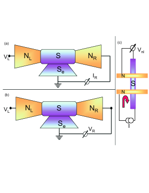
Figure 1: (Color online.) Sketch of a three-terminal device for (a) measurement of the non-local conductance and (b) measurement of the non-local resistance. (c) Typical experimental setup for measurement of the non-local resistance.

II The Model and basic equations

A typical experimental setup for the measurement of non-local transport properties is shown in Fig. 1c. On top of a nanoscale superconducting wire one places several (in our case two) normal wires. A current is injected from one of the normal electrodes and flows in the direction shown in the figure. The non-local resistance is then obtained by measuring the potential difference between the other normal electrode and the end of the superconducting wire through which no current is flowing. A strong enough non-local signal is measured when the distance between the normal leads does not exceed much the coherence length of the superconductor.

A self-consistent computation of the spatial variation of the gap and currents in such a device is a formidable task which we will not address here. Nevertheless, the mean features of the system can be described by considering the geometry shown in Figs. 1a and 1b. A superconducting region $S$ is connected to two normal electrodes N_L and N_R and to a superconducting electrode $S_{e}$, made of the same superconducting material as $S$. The three interfaces will be described by characteristic energies $\epsilon_{L}$,$\epsilon_{R}$ and $\epsilon_{S}$, defined below. As we are not interested in the spatial variation of the non-local correlations, we simplify the problem by assuming that the central superconducting region $S$ has dimensions smaller than the superconducting coherence length, which in the diffusive limit is given by $\xi_{S}=\sqrt{D/\Delta}$. Here $\Delta$ is the superconducting gap and $D$ is the diffusion coefficient. Thus, we may assume that the order parameter and the non-equilibrium distribution are uniform over $S$ .

In order to determine either the non-local conductance (Fig. 1a) or resistance (Fig. 1b) we need to calculate the current density ${\bf j}$ and the self-consistent order parameter $\Delta$ in the $S$ region. As one can see from our results below, we always find a stationary current state. This behavior is distinctive for junctions consisting of a mesoscopic superconductor in contact with a bulk onevolkov . Thus, ${\bf j}$ and $\Delta$ can be expressed in terms of the Keldysh component of the matrix GF $\check{g}$

$$\Delta = \frac{\lambda}{4}\int d\epsilon\hat{g}^{K}_{12}$$ (1)

$${\bf j} = \frac{1}{8eG_{N}}\int d\epsilon{\rm Tr}\left\{\hat{\tau}_{3}\check{g}\nabla\check{g}\right\}^{K}\;,$$ (2)

where $\lambda$ is the BCS coupling constant which determines the critical temperature, and $R_{N}$ is the normal state resistance of the $S$ region. The function $\check{g}$ is a 4$\times$4 matrix in the Nambu$\otimes$Keldysh space with the usual structure

$$\check{g}=\left(\begin{array}[]{cc}\hat{g}^{R}&\hat{g}^{K}\\ 0&\hat{g}^{A}\end{array}\right),$$ (3)

while $\hat{g}$ are 2$\times$2 matrices in Nambu space. In the diffusive limit these functions are the solutions of the Usadel equationusadel

$$-D\nabla(\check{g}\nabla\check{g})-i\epsilon\left[\hat{\tau}_{3},\check{g}\right]-i\left[\check{\Delta},\check{g}\right]=-i\left[\check{\Sigma}_{in},\check{g}\right]\;,$$ (4)

supplemented by the normalization condition $\check{g}^{2}=\check{1}$. Here $\check{\Sigma}_{in}$ is the self-energy term describing inelastic processes. In the time relaxation approach $\check{\Sigma}_{in}$ is proportional to $1/\tau_{in}$, where $\tau_{in}$ is the inelastic relaxation time. We will assume that $1/\tau_{in}$ is the smallest energy scale and neglect this term. At the interfaces with the electrodes we use the Kupryianov-Lukichev boundary conditionskl

$$D\check{g}\nabla\check{g}|_{\bf n}=\epsilon_{i}d\left[\check{g},\check{g}_{i}\right]\;,$$ (5)

where $\check{g}_{i}$ are the GF of the electrodes($i=L,R,S_{e}$), $\epsilon_{i}=\epsilon_{Th}/2r_{B}$, $\epsilon_{Th}=D/d^{2}$ is the Thouless energy, $r_{B}=R_{Bi}/R_{N}$, $R_{bi}$ is the ith barrier resistance per unit area, and ${\bf n}$ denotes a unit vector normal to the interface. We assume that the GFs of the electrodes remain unchanged and equal to the bulk values, i.e. $\hat{g}^{R(A)}=\pm\hat{\tau}_{3}$ in the normal leads, and $\hat{g}^{R(A)}_{S}=g^{R(A)}_{BCS}\hat{\tau}_{3}+f^{R(A)}_{BCS}i\hat{\tau}_{2}$ in the superconductor electrode, where $g^{R(A)}_{BCS}=\epsilon/\sqrt{(\epsilon\pm i\eta)^{2}-\Delta_{0}^{2}}$ and $f^{R(A)}_{BCS}=\Delta_{0}/\sqrt{(\epsilon\pm i\eta)^{2}-\Delta_{0}^{2}}$. While the Keldysh components are given by

$$\hat{g}^{K}_{i}=\hat{g}^{R}_{i}\hat{F}_{i}-\hat{F}_{i}\hat{g}^{A}$$ (6)

where

$$\hat{F}_{i}=F_{i+}\hat{\tau}_{0}+F_{i-}\hat{\tau}_{3},$$

$V_{i}$ is the voltage in electrode $i$ , and $F_{i\pm}=\frac{1}{2}\left[\tanh(\frac{\epsilon+eV_{i}}{2T})\pm\tanh(\frac{\epsilon-eV_{i}}{2T})\right]$ . We also assume that $V_{S_{e}}=0$. In principle the boundary conditions Eq. (5) are valid for low transmitting interfaces. In the present work we consider that the interface transparencies may vary in the range $10^{-3}-10^{-1}$ for which Eq. (5) is sufficiently reliable.

With the help of Eq. (5) we can calculate the total current at each interface using the expression:

$$eI_{i}R_{N}=\frac{\epsilon_{i}}{8\epsilon_{Th}}\int d\epsilon{\rm Tr\tau_{3}}\left[\check{g}_{i},\check{g}\right]^{K}\;.$$ (7)

In this case the GF inside S does not vary considerably and the Usadel equation (4) can be integrated over space coordinates using the boundary conditions Eq. (5). In this way one obtains a set of algebraic equations which can be written in a compact form

$$\left[\check{\Lambda},\check{g}\right]=0$$ (8)

where

$$\check{\Lambda}=\sum_{i=L,R,S}\epsilon_{i}\check{g}_{i}+\epsilon\tau_{3}+\check{\Delta}-\check{\Sigma}_{in}\;.$$

Eq. (8) is equivalent to the Nazarov’s circuit theory equations nazarov_ct , which were used in Refs. morten ; morten08 for nonlocal transport calculations. The solution for the R,A and K components of $\check{g}$ which satisfy Eq. (8) and the normalization condition can be formally be written as:

$$\hat{g}^{R(A)} = \frac{\hat{\Lambda}^{R(A)}}{\sqrt{\hat{\Lambda}^{R(A)}\hat{\Lambda}^{R(A)}}}$$ (9)

$$\hat{g}^{K} = \frac{\hat{\Lambda}^{K}-\hat{g}^{R}\hat{\Lambda}^{K}\hat{g}^{A}}{\sqrt{\hat{\Lambda}^{R}\hat{\Lambda}^{R}}+\sqrt{\hat{\Lambda}^{A}\hat{\Lambda}^{A}}}$$ (10)

Substituting these expressions into Eqs. (1-2) enable us to obtain numerically the self-consistent order parameter, the currents through the interfaces and the non-local voltage induced at the right electrode in the resistance measurement case.

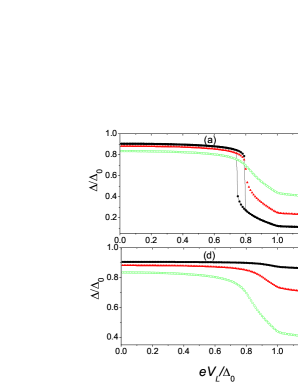
Figure 2: (Color online). The amplitude of the self-consistent order parameter, the current $I_{L}$ injected from the left normal electrode and the current $I_{R}$ measured at the right electrode, as a function of the voltage $V_{L}$. Panels (a)-(c) for $\epsilon_{S}=0.2$, $\epsilon_{L}=0.1$, $T=0.01\Delta_{0}$ and different values of $\epsilon_{R}$. Panels (d)-(f) for $\epsilon_{S}=0.2$, $\epsilon_{R}=0.1$, $T=0.01\Delta_{0}$ and different values of $\epsilon_{L}$. We have defined $R=R_{N}\epsilon_{Th}/\Delta_{0}$.

III Measurement of the non-local conductance

In this section we consider the experimental set-up of Fig. 1a. The left normal electrode is biased by a voltage source at $V_{L}$. For a non-local conductance measurement we will assume that the $N_{R}$ is grounded ($V_{R}=0$), and compute the current $I_{R}$ through the interface $S/N_{R}$ from Eqs. (7,9,10) and the self-consistent order parameter $\Delta$ from Eq. (1). Before we address the non-local properties of the system let us discuss the results concerning local properties.

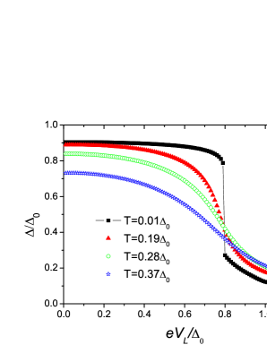
Figure 3: (Color online). The amplitude of the self-consistent order parameter as a function of the voltage $V_{L}$, for different temperatures. Notice that in the range of temperatures shown and for large values of $V_{L}$ the gap is enhanced by increasing $T$.

In Fig. 2a we show the amplitude of $\Delta$ as a function of the bias voltage $V_{L}$ for $\epsilon_{S}=0.2\Delta_{0}$, $\epsilon_{L}=0.1\Delta_{0}$ and three different values of $\epsilon_{R}=0.01-0.1$, corresponding to transmission coefficients in the range $10^{-3}-10^{-2}$ (we assume that the length of the superconducting region is about $50nm$). All energies are given in units of $\Delta_{0}$, which is the value of the order parameter in the bulk at $T=0$. For a fixed low value of $V_{L}$, $\Delta$ is reduced by increasing the coupling with the right normal electrode, which is a consequence of the inverse proximity effect. At some value $V_{L}^{*}\simeq 0.8\Delta_{0}$ of the order of the self-consistent $\Delta$, one can see an abrupt reduction of the self-consistent order parameter. For voltages larger than $V_{L}^{*}$ the quasi-particle current through $S$ becomes considerably larger (Figs. 2b and 2c), i.e. the system is driven out of equilibrium. An interesting consequence of this non-equilibrium state for voltages $V_{L}>\sim V_{L}^{*}$ is the enhancement of the self-consistent gap by increasing the temperature, as shown in Fig. 3. This effect is related to the stimulation of superconductivity by quasiparticle currents in SIS systems, and was studied both theoreticalzaitsev91 and experimentallyblamire .

From Fig. 2a one can also see that the suppression of $\Delta$ at $V_{L}^{*}$ becomes more abrupt the weaker the coupling with the right electrode is. Figures 2b and 2c also show the corresponding current at the left and right interfaces. As expected the larger the resistance of the right interface (small $\epsilon_{R}$) the smaller the value of $I_{R}$. A strong non-equilibrium situation takes place when most of the current injected flows into the superconducting electrode, i.e. when $\epsilon_{R}$ is small enough (in our example $\epsilon_{R}=0.01$). In this case the gap becomes multivalued and this is reflected in the behavior of the currents $I_{L}$ and $I_{R}$. Multivalued solutions for the self-consistent gap were also found in Ref.zaitsev91 for SIS systems and recently in Ref.nazarov for a NSN system.

Another interesting feature of this system is the existence of a region of voltages for which the local conductance is negative (see Fig. 2b). This behavior was also obtained in Ref. volkov for a system consisting of a superconducting link separating a normal and a superconducting electrode. Also in Ref.prb09 negative local conductance was obtained for a two dimensional ballistic superconductor attached to two normal electrodes. Notice however, that the part of the curve corresponding to a negative conductance would be not accessible in current biased experiments. If we now fix the value of $\epsilon_{R}$ at its maximum value $\epsilon_{R}=0.1$ and vary $\epsilon_{L}$, we see that even for the smallest coupling ($\epsilon_{L}=0.01\Delta_{0}$) the variation of the gap and the currents is smooth and no signatures of multivalued solutions appears for this range of parameters (see bottom row of Fig. 2).

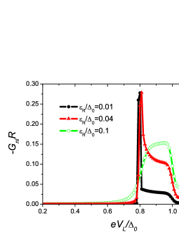
Figure 4: (Color online). The voltage dependence of the (negative) non-local conductance $G_{nl}$ normalized with respect to $R=R_{N}\epsilon_{Th}/\Delta_{0}$. We have chosen $T=0.01\Delta_{0}$, $\epsilon_{S}=0.2$, $\epsilon_{L}=0.1$, $T=0.01\Delta_{0}$ and different values of $\epsilon_{R}$ .

Let us now focus on the non-local transport and compute the non-local conductance, which can be obtained easily from the knowledge of $I_{R}$ (Fig. 2c and 2f) . It is given by the expression

$$G_{nl}=\frac{\partial I_{R}}{\partial V_{L}}\;.$$ (11)

and shown in Fig. 4 as a function of the bias voltage $V_{L}$, for different values of the coupling energies $\epsilon_{L,R}$. In all cases $G_{nl}$ is very small in the region of low voltages. This is in agreement with the zero non-local conductance obtained in the lowest order of tunnelingfalci , due to the cancellation of the EC and CAR processes. However, our results are in all order of tunneling and therefore a dominance of EC (negative $G_{nl}$) is obtained in accordance to Ref. regis . For voltages of the order of the self-consistent $\Delta$, the value of $G_{nl}$ becomes significant. However, no change of sign is observed. As mentioned in the introduction, non-interacting models do not exhibit a change of sign of the non-local conductance in three-terminal NSN structures. This can only be achieved when electron-electron interactions are taken into accountnatphys .

IV Measurement of the non-local resistance in a three-terminal device

In a real experiment it is easier to measure a voltage rather than a current. Indeed the experiments of Refs. beckmann ; chan ; delft ; beckmann2 ; basel were performed in (a) the current biased regime and (b) instead of the current, the non-local resistance (or voltage) was measured. Theoretically, it is not simple to impose a current bias. Therefore we will still work in the voltage biased case but determine the induced non-local voltage and resistance imposing zero current at the $S/N_{R}$ interface. Thus, all the current injected from the left normal electrode flows into the superconducting electrode $S_{e}$ (see Fig. 1b). The current at the right interface is given by (cf. Eq.(7)):

$$eI_{R}R_{BR}=\frac{1}{8}\int d\epsilon{\rm Tr}\hat{g}^{K}(\epsilon)-\frac{1}{4}\int d\epsilon\nu_{s}(\epsilon)\left(\tanh(\frac{\epsilon+eV_{R}}{2T})-\tanh(\frac{\epsilon-eV_{R}}{2T})\right)\;,$$ (12)

where $\nu_{s}(\epsilon)=(g^{R}-g^{A})/2$ is the density of states of S and $R_{BR}$ is the $R$ barrier resistance per unit area. The first term in the r.h.s is proportional to the quantity $Q^{*}$ identified in the literature as the charge imbalance potentialci , which appears due to a non-equilibrium distribution in the superconductor. The second term is the usual quasiparticle current term. The voltage $V_{R}$ is measured with respect to the ground (see Fig. 1b) and it is obtained by imposing $I_{R}=0$.

The results for $\Delta$, the injected current $I_{L}$ and the induced voltage $V_{R}$ as a function of the bias voltage $V_{L}$ are shown in Fig. 5, for fixed values of $\epsilon_{S,L}$ and different values of $\epsilon_{R}$ in the same range as in Fig. 2. In the case of low values of $\epsilon_{R}$, the self-consistent gap has a very similar behavior as in the preceding section. However, for the largest value $\epsilon_{R}=0.1\Delta_{0}$ the suppression of $\Delta$ is larger as the one obtained by imposing $V_{R}=0$. Notice also that the region of negative local conductance (Fig. 5b), associated with the abrupt change of the order parameter appears now for all values of $\epsilon_{R}$. It is clear that by having imposed $I_{R}=0$ all the current injected must flow through the $S/S_{e}$ interface and our system behaves similarly to the $N/S/S$ studied in Ref.volkov . In Fig. 5c we also show the voltage $V_{R}$ induced in the right electrode calculated by equalizing (12) to zero. At low $V_{L}$ values the induced voltage $V_{R}$ is very small, but it experiences a jump at the value of $V_{L}$ where the self-consistent gap exhibits its maximal drop.

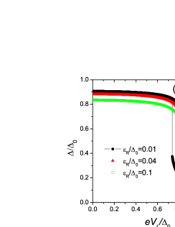
Figure 5: (Color online). The amplitude of the self-consistent order parameter (a), the current $I_{L}$ injected from the left normal electrode (b) and the induced voltage $V_{R}$ measured at the right electrode (c), as a function of the voltage $V_{L}$, for $\epsilon_{S}=0.2$, $\epsilon_{L}=0.1$, $T=0.01\Delta_{0}$ and different values of $\epsilon_{R}$.

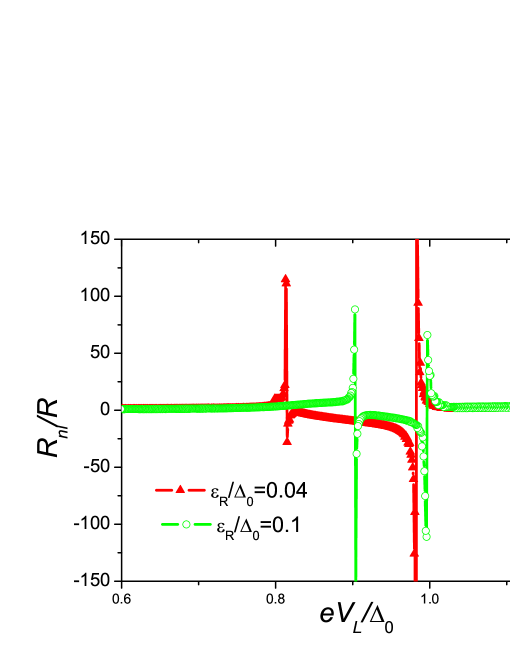
Figure 6: (Color online). The voltage dependence of the non-local resistance calculated from Eq.(13) for $\epsilon_{S}=0.2\Delta_{0}$, $\epsilon_{L}=0.1\Delta_{0}$, $T=0.01\Delta_{0}$, and two values of $\epsilon_{R}$.

We have now all quantities required to compute the non-local resistance which would be measured. This can be calculated from the expression:

$$R_{nl}=\frac{\partial V_{X}}{\partial I_{L}}=\frac{\partial V_{X}}{\partial V_{L}}\left(\frac{\partial I_{L}}{\partial V_{L}}\right)^{-1}\;.$$ (13)

The measured voltage $V_{X}$ depends on the experimental set-up. We are considering here the three-terminal structure of Fig. 1b, and determining $V_{R}$ respect to the ground. Thus in this case $V_{X}=V_{R}$, i.e. the one shown in 5c. According to Eq. (13) there are two factors determining the non-local resistance. One which is the inverse of the local conductance $G_{LL}^{-1}=dV_{L}/dI_{L}$ and which decrease by increasing $\epsilon_{L}$. The second contribution is given by $dV_{R}/dV_{L}$ which is nonzero only if a non-equilibrium distribution appears in the $S$ region and is related to the charge imbalance term (cf. Eq. (12)).

In Fig. 6 we show the dependence $R_{nl}(V_{L})$ for two values of $\epsilon_{R}$ and $\epsilon_{L}=0.1\Delta_{0}$, $\epsilon_{S}=0.2\Delta_{0}$, $T=0.01\Delta_{0}$. The change of sign of $R_{nl}$ is a consequence of the negative local conductance which appears between the values $V_{L}\simeq 0.8\Delta_{0}$ and $V_{L}\simeq\Delta_{0}$ (see Fig. 5b). The position of the first peak of $R_{nl}$ is determined by the value of $V_{L}$ at which $\Delta$ drops substantially, while the position of second peak is determine by $\Delta_{0}$. As mentioned above, in current bias experiments the curve $R_{nl}$ may look very different to the ones shown in Fig. 6, since the region of negative local conductance may not be observed.

In experiments as those of Refsbeckmann ; chan ; basel the current flows along a superconducting wire, while in our model it flows into the reservoir $S_{e}$. For simplicity we have assume that the latter remains unaltered for all values $V_{L}$ considered here. In particular the value of the gap is the bulk BCS one for any value of $V_{L}$. However, in the experiments, when the current flowing through the wire reaches the critical value the superconducting gap is suppressed homogeneously in the region where the current is flowing.This leads to the observation of only one peak in the non-local resistancechan . In the next section we will model this situation.

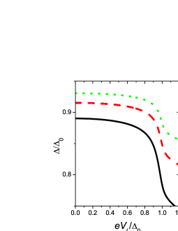
Figure 7: (Color online). The amplitude of the self-consistent order parameter, the current $I_{L}$ injected from the left normal electrode and the induced voltage $V_{R}$ measured at the right electrode, as a function of the voltage $V_{L}$, for $\epsilon_{L}=\epsilon_{R}=0.1$, $T=0.01\Delta_{0}$ and different values of $\epsilon_{S}$.

We should also emphasize that the change of sign of the non-local resistance obtained in Fig. 6 is due to the fact that the local conductance $G_{LL}=dI_{L}/dV_{L}$ becomes negative for some values of $V_{L}$ (cf. Fig. 5b). If the coupling $\epsilon_{S}$ is large enough, the local conductance remains always positive and so the non-local resistance. This is shown in Fig.7, where the amplitude of the self-consistency gap, the current injected and the voltage induced at the right electrode are plotted as a function of $V_{L}$, for $\epsilon_{S}=1,1.5$ and $2\Delta_{0}$. If one compares these results with those obtained for a smaller $\epsilon_{S}$ (Fig. 5), one sees that $\Delta$ is now only weakly suppressed and that the current $I_{L}$ increases monotonically. Thus the non-local resistance is always positive as it shown in Fig. 8.

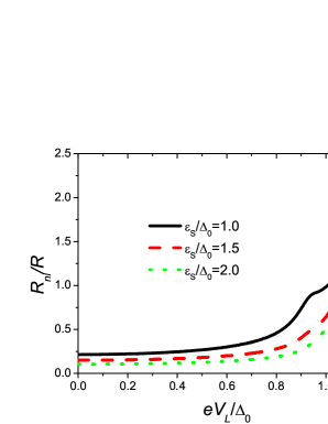
Figure 8: (Color online). The voltage dependence of non-local resistance for the same parameters as in Fig. 7 .

Finally, we show in Fig. 9 the temperature dependence of the zero bias non-local resistance for different values of the coupling parameter $\epsilon_{S}$. We can see that while for the small values of $\epsilon_{S}$ the non-local resistance increases monotonously with the temperature, for larger values of $\epsilon_{S}$, $R_{nl}$ reaches a maximum value. In the latter case the charge imbalance effect becomes important and dominates over the local conductance factor for large temperatures. This behavior is in agreement with previous calculations of $R_{nl}$ in a superconducting quantum dot golubev . One could conclude as in Refzaikin09 that the non-monotonic behavior of $R_{nl}(T)$ is in qualitative agreement with the observations of Refs.beckmann ; chan . However, we hardly believe that. If this would be the case then one should obtain for the same parameter range a change of sign for $R_{nl}$ as a function of the injected current, as observed in the experimentschan . On the contrary, Fig. 8 clearly shows a monotonic increase of $R_{nl}$ with the applied voltage. In the next section we will show that the change of sign of $R_{nl}$ observed in the experiment is due to the suppression of the superconductivity by the injection of a current. Also the peak of $R_{nl}$ observed as a function of temperature could be understood within this model.

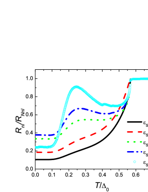
Figure 9: (Color online). The temperature dependence of the zero bias non-local resistance measure in a three terminal device for different values of $\epsilon_{S}$. We have chosen $\epsilon_{L}=\epsilon_{R}=0.1\Delta_{0}$

V Four terminal structure

We now consider a situation closer to that of the experiments of Ref.chan ; basel , in which the non-local resistance (voltage) has been measured in a multi-terminal setup consisting of a superconducting wire attached to several normal terminals. In these experiments the nonlocal voltage corresponds to the potential difference between one end of the superconducting wire and one of the normal leads.

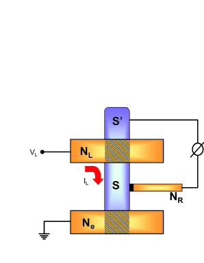
Figure 10: (Color online). Sketch of the 4-terminal structure under consideration.

We model these experimental situations as shown in Fig. 10. On the top of a superconducting wire we place two normal contacts. A current flows from the $N_{L}$ contact to the $N_{e}$ due to the bias voltage $V_{L}$ applied between the contacts. We are interested in the voltage difference measured between the end of the wire, which we denote by $S^{\prime}$, and an additional normal contact $N_{R}$. We use on purpose the same notation as in Fig. 1 in order to use straightforwardly the expressions derived in section II. The only difference is that the drain electrode is now in the normal state and that we measure the voltage difference between the end $S^{\prime}$ of the superconducting slab and the normal electrode $N_{R}$. The electrode $N_{e}$ is grounded. In order to compute the resistance measured between $S^{\prime}$ and $N_{R}$ we proceed as in the last section, determining the Green functions from Eqs. (9-10) and the self-consistent gap. Now we impose that the currents through the $S/N_{R}$ and through the $S/S^{\prime}$ interfaces are zero. The current trough the $S/S^{\prime}$ interface can be written as the sum

$$I_{S/S^{\prime}}=I_{J}+I_{qp}\;$$ (14)

of the Josephson and the quasiparticle contribution respectively. The first is given by the product of anomalous Green’s functions in Eq. (2) while the latter by the product of normal components. Since no current is flowing into $S^{\prime}$ we assume that there the Green’s functions are those in equilibrium, with $|\Delta|$ equal to the self-consistent $|\Delta|$ in the S region at $V_{L}=0$, and a phase $\phi$ which is determined by imposing the condition of no current through the $S/S^{\prime}$ interface. For voltages lower than a critical voltage $V_{L}^{*}\sim\Delta$ we always found a finite value of $\phi$. In this case the voltage $V^{\prime}$ induced in $S^{\prime}$ equals zero, and the measured $V_{nl}$ coincides with $V_{R}$ of the previous section. The voltage $V_{L}^{*}$ is the voltage at which the self-consistent gap vanishes, i.e. when the current flowing in $S$ reaches its critical value. For values of $V_{L}$ larger than this value the quasiparticle current becomes finite, and a voltage $V^{\prime}$ is induced in $S^{\prime}$. We compute it from an expression obtained by equalizing Eq.(7) to zero. Thus, the non-local resistance is given by Eq. (13) where now $V_{X}=V_{R}$ for $V_{L}<V_{L}^{*}$ and $V_{X}=V_{R}-V^{\prime}$ for $V_{L}>V_{L}^{*}$. In Fig. 11 we show the result of our calculation for $R_{nl}$ as a function of $V_{L}$. It shows a peak at $V_{L}^{*}$. Since the latter is of the order of $\Delta$, the peak is shifted to lower voltages by increasing the temperature (Fig. 11) . This behavior is in agreement with the experimental observation of Ref. chan , where the peak occurred at values of the bias current close to the value of critical current of the superconducting wire. The change of sign of $R_{nl}$ is related to the non-equilibrium situation created in $S$ by the injection of a current from $N_{L}$. We also show in the inset of Fig. 11 the temperature dependence of $R_{nl}$, which exhibits a pronounced peak for $V_{L}\simeq V_{L}^{*}$. This is again in agreement with the observations of Ref.chan . These results demonstrate that the model studied here contains the main ingredients for describing experiments on non-local transport as the one of Ref.chan . Within this model the change of sign of the non-local resistance has its origin in the deviation of the distribution function of the superconductor from the equilibrium one. Notice, that as in Ref.chan , the change of sign of $R_{nl}$ occurs at the critical current which corresponds to the voltage $V_{L}^{*}$ in our model.

In other experimentsdelft ; basel , however, the change of sign occurred at lower voltages. This discrepancy is at the moment not clarified and may be related to the inclusion of electron-electron interactions as proposed in Ref.natphys .

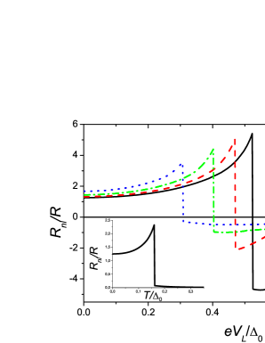
Figure 11: (Color online). The non-local resistance measured in a four terminal structure as a function of the bias voltage $V_{L}$ for $\epsilon_{L}=\epsilon_{R}=0.1\Delta_{0}$, $\epsilon_{S}=0.2$, and different values of the temperature. Inset: The non-local resistance as a function of the temperature at zero bias.

VI Conclusions

We have presented a self-consistent analysis of the transport properties of a structure consisting of a mesoscopic superconductor whose dimensions are smaller than the characteristic length $\xi_{S}$, attached to two normal and one superconducting terminals. We have analyzed two measurement methods: one in which the detector (R) electrode is grounded and the leaking current is measured, and one in which the current through this lead is fixed to zero and the induced voltage is measured. In both cases we observe that the self-consistent order parameter in the mesoscopic central region exhibits an abrupt drop at a certain voltage of the order of the self-consistent $\Delta$. Associated to this drop the local differential conductance at the injector lead (L) may become negative for certain values of the coupling parameters, resulting in a change of sign of the non-local resistance. As we stress throughout this manuscript, this change of sign would not be related to a dominance of CAR over EC processes but to a non-equilibrium effect. We have still described another mechanism for the appearance of negative non-local resistance which is probably most suitable for explaining the observations of Ref. chan . This mechanism is applicable in a four terminal geometry and corresponds to the injection of large currents which may switch the superconducting region into the normal state. The observation of a change of sign in the non-local signal at smaller bias and small transparencies like the ones reported in Refs. delft ; basel are certainly not possible to be explained with the theoretical model presented in this work and might be related to the influence of electron-electron interactions, as already pointed out in Ref. natphys . Further work for analyzing the combined effect of interactions and non-equilibrium effects is under progress.

References

- (1) D. Beckmann, H.B. Weber and H. v. Löhneysen, Phys. Rev. Lett. 93, 197003 (2004).
- (2) S. Russo, M. Kroug, T.M. Klapwijk and A.F. Morpurgo, Phys. Rev. Lett. 95, 027002 (2005).
- (3) P. Cadden-Zimansky and V. Chandrasekhar, Phys. Rev. Lett. 97, 237003 (2006); P. Cadden-Zimansky, Z. Ziang and V. Chandrasekhar, New J. Phys. 9, 116 (2007).
- (4) D. Beckmann and H. v. Löhneysen, Applied Physics A 89, 603 (2007).
- (5) A. Kleine, A. Baumgartner, J. Trbovic and C. Schöeneberger, cond-mat-01812.3553v2 (2009).
- (6) A.F. Andreev, Zh. Eksp. Teor. Fiz. 46, 1823 (1964) [Sov. Phys. JETP 19, 1228 (1964)].
- (7) J. M. Byers and M. E. Flatté, Phys. Rev. Lett. 74, 306 (1995).
- (8) G. Falci, D. Feinberg, and H. Hekking, Europhys. Lett. 54, 255 (2001).
- (9) R. Mélin and D. Feinberg, Phys. Rev. B 70, 174509 (2004); S. Duhot and R. Mélin, Eur. Phys. J. B 53, 257 (2006); R. Mélin, Phys. Rev. B 73, 174512 (2006).
- (10) M.S. Kalenkov and A.D. Zaikin, JETP Lett. 87, 140 (2008) [Pis’ma v ZhETF, 87, 166 (2008)].
- (11) J.P. Morten, A. Brataas and W. Belzig, Phys. Rev. B 74, 214510 (2006).
- (12) A. Brinkman abd A.A. Golubov, Phys. Rev.B 74, 214512 (2006).
- (13) D. S. Golubev and A. D. Zaikin, Phys. Rev. B 76, 184510 (2007).
- (14) R. Melin, F. S. Bergeret, A. Levy Yeyati, Phys. Rev. B 79, 104518 (2009).
- (15) D.S. Golubev, M.S. Kalenkov, A.D. Zaikin, arXiv:0904.3455.
- (16) A. Levy Yeyati, F.S. Bergeret, A. Martin-Rodero and T.M. Klapwijk, Nature Phys. 3, 455 (2007).
- (17) K.D. Usadel, Phys. Rev. Lett. 25, 507 (1970).
- (18) M. Kupriyanov and V. F. Lukichev, Sov. Phys. JETP 67, 1163 (1988).
- (19) D. Feinberg, Eur. Phys. J. B 36, 419 (2003).
- (20) A. V. Zaitsev, JETP Lett. 55,67 (1991).
- (21) M. G. Blamire, E. C. G. Kirk, J. E. Evetts and T. M. Klapwijk, Phys. Rev. Lett. 66, 220 (1991).
- (22) Yu. V. Nazarov, Superlatt. Microstruct. 25, 1221 (1999).
- (23) J. P. Morten, D. Huertas-Hernando, W. Belzig, and A. Brataas, Phys. Rev. B 78, 224515 (2008).
- (24) I. Snyman and Yu. V. Nazarov, Phys. Rev. B 79, 014510 (2009).
- (25) M. S. Kalenkov and A. D. Zaikin, Phys. Rev. B 75, 172503 (2007).
- (26) A. V. Zaitsev, A. F. Volkov, S. W. Bailey, and C. J. Lambert, Phys. Rev. B 60, 3559 (1999).
- (27) J. Clarke, Phys. Rev. Lett. 28, 1363 (1972); M. Tinkham and J. Clarke, Phys. Rev. Lett. 28, 1366 (1972).