A New Scaling Law on Throughput and Delay Performance of Wireless Mobile Relay Networks over Parallel Fading Channels

Abstract

In this paper, utilizing the relay buffers, we propose an opportunistic decode-wait-and-forward relay scheme for a point-to-point communication system with a half-duplexing relay network to better exploit the time diversity and relay mobility. For instance, we analyze the asymptotic throughput-delay tradeoffs in a dense relay network for two scenarios: (1) fixed relays with microscopic fading channels (multipath channels), and (2) mobile relays with macroscopic fading channels (path loss). In the first scenario, the proposed scheme can better exploit the multi-relay diversity in the sense that with $K$ fixed relays and a cost of $\mathcal{O}(K)$ average end-to-end packet delay, it could achieve the same optimal asymptotic average throughput as the existing designs (such as regular decode-and-forward relay schemes) with $K^{2}$ fixed relays. In the second scenario, the proposed scheme achieves the maximum throughput of $\Theta(\log K)$ at a cost of $\mathcal{O}(K/q)$ average end-to-end packet delay, where $0<q\leq\frac{1}{2}$ measures the speed of relays’ mobility. This system throughput is unattainable for the existing designs with low relay mobility, the proposed relay scheme can exploit the relays’ mobility more efficiently.

I Introduction

In wireless communication networks, cooperative relaying not only extends the coverage but also contributes the spatial diversity. As a result, cooperative relay is one of the core technology components in the next generation wireless systems such as IEEE 802.16m and LTE-A. Extensive research is being carried out on the theory and algorithm design of cooperative relay and there are still a lot of open issues associated with the capacity and the design of relay networks. For instance, most of the existing works on relay protocol designs have ignored and failed to exploit the buffer dynamics in the relay. As such, how could the throughput of relay networks benefit from the mobility of relays is still not clearly known and we shall try to shed some lights on this aspect in this paper. Specifically, utilizing buffers in the relays, an opportunistic decode-wait-and-forward (ODWF) relay scheme is proposed to exploit the mobility of relays so as to improve the system throughput of the mobile relay networks. Moreover, the asymptotic tradeoff of the end-to-end packet delay versus the end-to-end throughput of the ODWF scheme is analyzed to obtain the design insights.

I-A Related Work

The initial study of relay channels can be traced back to 1970s [1, 2, 3]. The capacity of the relay channel consisting of single source, destination and relay station was derived by Cover and El Gamal in [4]. Since then, different types of relay channels have been investigated from the information theoretic perspective, including the relay-assisted point-to-point communication [5, 6, 7], relay broadcasting channels in [8, 9, 10], multi-source multi-destination relay channels [9, 11, 12]. Recent research mainly focuses on two topologies of wireless relay (or multi-hop) networks, namely ad hoc networks and relay-assisted point-to-point communications. In wireless ad hoc networks, any pair of nodes are allowed to communicate; in relay-assisted point-to-point communications, there exists only one pair of source and destination while other nodes serve as relay stations. The scaling law of the wireless ad hoc network capacity is first studied by Gupta and Kumar in [13]. Specifically, it is shown that each node can achieve the throughput of the order $\mathcal{O}(\frac{1}{\sqrt{K\log K}})$ when $K$ fixed nodes are randomly distributed over a unit area. The same throughput bound is also obtained in [14, 15, 16] by other approaches. Later, in [17] the throughput of the order $\mathcal{O}(\frac{1}{\sqrt{K}})$ is shown to be achievable, and in [18] the throughput order is enhanced to $\mathcal{O}(\frac{1}{K^{\frac{1}{3}}})$. These results imply that the throughput of each node converges to zero when the number of nodes increases. Nevertheless, it’s found in [19] that the per-node throughput can arbitrarily close to constant by hierarchical cooperation, and in [20] that the constant per-node throughput is achievable by exploiting the node mobility. In addition, in [14, 15] the throughput-delay tradeoff of wireless ad hoc networks is studied as the gain on network throughput is obtained at the expense of packet delivery delay.

The design of point-to-point communication via relay networks differs from that of wireless ad hoc networks in that there is only one data stream in the system and the system objective is to maximize single-link throughput, rather than the throughput of the weakest source-destination pair (in wireless ad hoc networks). Hence, it’s expected that the relay-assisted point-to-point communications could achieve higher per-node throughput than ad hoc networks. In [21, 22], it’s shown that the source-destination throughput can scale as $\log K$ when all the relays amplify and forward the received packet to the destination cooperatively with $\Theta(K)$ total transmission power. This relay strategy was extended to the case of multiple antennas in [23], where the throughput can scale as $\frac{M}{2}\log K$ with $M$ antennas at both the source and the destination. The throughput scaling with $\Theta(\log K)$ as derived in prior works can be interpreted as follows: since all the relay nodes should amplify and forward the received packets, the total transmit power of the relay network is $\Theta(K)$, then by Shannon’s capacity theory the throughput is $\Theta(\log K)$.

I-B Contributions

In this paper, we shall extend the existing knowledge on the point-to-point communications with relay networks in the following aspects.

• By exploiting the mobility of relay nodes through our proposed ODWF scheme, the asymptotical throughput $\Theta(\log K)$ is also achievable even with $\Theta(1)$ total transmit power and decode-and-forward relays. Moreover, compared with the constant per-node throughput (achieved by exploiting the relays’ mobility) in [20], our work shows that if there is only one data stream in the system, the source can transmit with a much higher date rate with the assistance of other relays.

• Even if the relays are fixed, the ODWF scheme can better exploit the multi-relay diversity, therefore, achieving higher throughput than the existing designs.

Specifically, we propose an opportunistic decode-wait-and-forward (ODWF) relay scheme which utilizes relay buffers to exploit the mobility of relays in a point-to-point communication link assisted by $K$ mobile relays with $N$ parallel fading channels (e.g. OFDM systems). In this scheme, only one of the relays is selected at any time to forward packets to the destination. The key feature of the proposed scheme is that the phase I (source to relay) and phase II (relay to destination) transmissions are scheduled based on the instantaneous channel states rather than having phase I and phase II as inseparable atomic actions (phase II always follows immediately from phase I) as in the existing designs, which is illustrated in Fig.1. By exploiting the mobility of relays in the phase I and phase II scheduling, we could achieve a better throughput scaling law. Moreover, we also examine the performance of the ODWF scheme in fixed relay networks, and it’s shown that the ODWF scheme could better exploit the multi-relay diversity than the existing designs even without relay mobility. In the proposed ODWF scheme, packets may have to be buffered at the relay nodes when phase II transmission cannot be scheduled immediately. As a result, we shall quantify the scaling law of the throughput-delay tradeoff in two scenarios, namely the fixed relays with microscopic fading (multipath fading) as well as the mobile relays with macroscopic fading (path loss). As comparisons, we also derive the throughput of the existing relay schemes (i.e. regular decode-and-forward schemes) in both scenarios as a performance baseline. In the scenario of fixed relays with microscopic fading, the proposed ODWF scheme exploits the time diversity of the multipath channels by scheduling the phase I and phase II transmissions adaptively. For this scenario, the proposed scheme can achieve the following performance:

• The achievable average system throughput is $\frac{N}{2}\log_{2}\left[1+p\ln K\right]$, which is higher than $\frac{N}{2}\log_{2}\left[1+p\ln\sqrt{K}\right]$ achieved by the existing regular decode-and-forward scheme for $K$ fixed relays, where $p$ is transmit power and $N$ is number of subcarriers.

• The average system throughput $\frac{N}{2}\log_{2}\left[1+p\ln\beta\right]$ can be achieved at a cost of $\frac{\beta^{2}}{K}$ average end-to-end packet delay, where $\beta\sim\mathcal{O}(K)$.

On the other hand, in the scenario of mobile relays with macroscopic fading, the ODWF scheme exploits the relay mobility by scheduling the phase I and phase II transmissions and it can achieve the following performance:

• The proposed scheme achieves a higher throughput scaling of $\frac{N\alpha}{4}\log_{2}K$ compared with the regular decode-and-forward schemes. The throughput gain over the regular schemes is $\mathbf{\Theta}\left(\frac{\log_{2}K}{qK^{\frac{1}{M-1}}}\right)$ when the relays’ velocity $q$ is small (e.g. $q=\frac{1}{K}$), where $\alpha$ is the pathloss exponent, $N$ is the number of subcarriers, $M>1$ is an integer related to the relays’ mobility model.

• The average system throughput $\frac{N}{2}\log_{2}\beta$ can be achieved at a cost of $\mathcal{O}(\max\{\frac{1}{q},\frac{\beta^{\frac{4}{\alpha}}}{Kq}\})$ average end-to-end packet delay, where $\beta\sim\mathcal{O}(K^{\frac{\alpha}{2}})$.

The remaining of this paper is organized as follows. In Section II, the system models for both fixed relays and mobile relays scenarios are introduced. In Section III, the ODWF scheme for fixed relays scenario is described, followed by the throughput-delay tradeoff analysis. In Section IV, the ODWF scheme for mobile relays scenario as well as the related throughput-delay tradeoff analysis is presented, followed by the conclusions in Section V.

II System Model

In this section, we shall describe the system models for both fixed relays and mobile relays scenarios, and define the performance metrics.

II-A System Model for Fixed Relays with Microscopic Fading

In the scenario of fixed relays, a cluster of $K$ fixed relay nodes lies between the source and the destination, as shown in Fig. 2. The path loss of all source-relay and relay-destination links are assumed identical. The OFDM technology is used for converting the frequency selective channel into $N$ parallel flat fading channels (subcarriers). There is no direct link between the source and destination due to the long distance and hence the source could only rely on the relay network for forwarding its packets to the destination (as in [22]). The relay strategy we consider is decode-and-forward (DaF) [4], and all the relays are half-duplexing. Moreover, at most one relay is selected at any time on each subcarrier. To facilitate the relay scheduling, transmission is partitioned into frames. As illustrated in Fig. 3, each frame is further divided into three types of slots defined as follows:

• Channel Estimation Slot is used by relays for estimating the channel gains with the source and destination.

• Control Slot is used by relays for distributive control signaling of the ODWF scheme. The details is given in the scheme description.

• Transmission Slot is used for data transmission.

Physical Layer Model

We shall model the physical layer performance by means of mutual information. Such an approach decouples the implementation details (coding and modulation) of the PHY layer and moreover, it has been demonstrated that strong coding such as LDPC code can achieve the Shannon’s capacity to within $0.05$dB with reasonable block size (e.g. 2k bytes) and target PER of $10^{-3}$. The maximum mutual information between the source and the $j$th relay on the $n$th subcarrier is given as

$$C^{s,j}_{n}=\log_{2}(1+p|H^{s,j}_{n}|^{2}),\\$$

and that between the $j$th relay and the destination on the $n$th subcarrier is given as

$$C^{j,d}_{n}=\log_{2}(1+p|H^{j,d}_{n}|^{2}),\\$$

where $p$ is the transmit power on each subcarrier, $H^{s,j}_{n}\sim\mathcal{CN}(0,1)$ and $H^{j,d}_{n}\sim\mathcal{CN}(0,1)$ are the microscopic fading gains (due to Rayleigh fading), and the effect of path loss is neglected as it’s identical for all links. All the packets are transmitted at data rate $r$. The $j$th relay could correctly decode the packets received over the $n$th subcarrier from the source only if $r\leq C^{s,j}_{n}$, and the destination could correctly decode the packets received over the $n$th subcarrier from the $j$th relay only if $r\leq C^{j,d}_{n}$. For convenience, we shall call a link as a connected link if its maximum mutual information is larger than $r$, and otherwise a broken link.

II-B System Model for Mobile Relays with Macroscopic Fading

In the scenario of mobile relays, we also consider a point-to-point communication system with $K$ relays and $N$ subcarriers. However, in this scenario, the relays are moving and the frame duration (the length of channel codeword) is much larger than that in the fixed relay scenario in order to capture the relays’ mobility. Therefore, we highlight in the following the differences of the system model for mobile relay networks from that for fixed relay networks discussed in the preceding part.

Relay Mobility Model

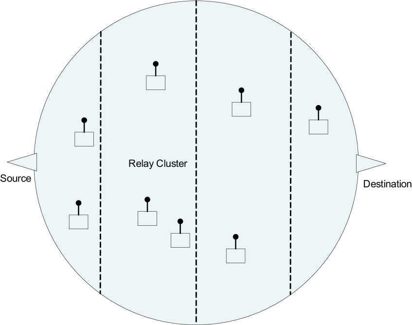
Figure 4: System model of the macroscopic fading scenario

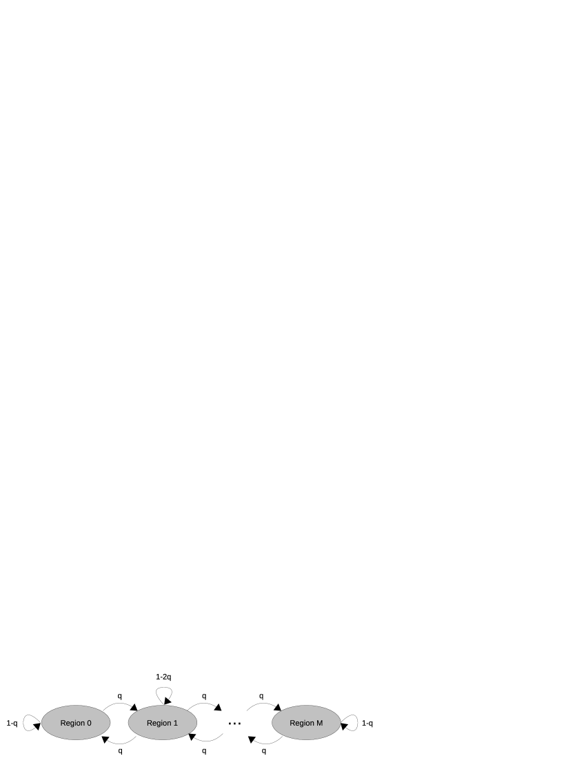
Figure 5: The random walk of each relay.

Following [13, 22], we assume that the $K$ relays are distributed on a disk with radius $R$ as illustrated in Fig. 4. The source and the destination are fixed at two ends of a diameter, and the disk is divided horizontally into M equal-area regions along the source-destination diameter. These regions are denoted as region 1, region 2, …, and region M, from the source to the destination. As illustrated in Fig. 5, the movement of each relay is modeled as a random walk (Markov chain) on these regions:

• At the beginning, each relay is uniformly distributed on the disk. Movements of relays can only occur in discrete frame with time index $t$.

• Let $X_{k}(t)$ denote the region index of the $k$th relay in the $t$th frame, $\{X_{k}(t)|t=1,...+\infty\}$ is a Markov chain with the following transition matrix

  $$Q_{i,j}=\left\{\begin{array}[]{ll}q&j=i+1\ \mbox{and}\ i=1,...,M-1\\ q&j=i-1\ \mbox{and}\ i=2,...,M\\ 1-2q&j=i=2,...,M-1\\ 1-q&j=i=1\mbox{ or }M\\ 0&\mbox{otherwise}\end{array}\right.$$ (1)

  where $Q_{i,j}$ denotes the transition probability that one relay jumps into the $j$th region in the next frame, providing that it is in the $i$th region currently.

• When one relay moves into a region, its actual location in this region is uniformly distributed.

Remarks: The region transition probability $q$ measures how likely one relay will move into another region in the next frame, and therefore, it is related to the average speed of the relays.

Physical Layer Model

In order to capture the dynamics of macroscopic fading (relays’ mobility), we assume the frame duration is much larger than the coherent time of the microscopic fading. As a result, the transmitter can deliver packets with the ergodic capacity (averaged over multipath fading) on every subcarrier in every frame. Since for one transmitter-receiver pair the ergodic capacity of different subcarriers is identical, it’s of less interests to consider different scheduling on different subcarriers. Hence, we assume each transmitter (source or relay) will use the whole spectrum when it’s transmitting packets, and each packet is jointly encoded across all subcarriers. Let $p$ be the transmit power on each subcarrier, the ergodic capacity between the source and the $j$th relay is given by

$$C^{s,j}=\mathbf{E}\left[\sum_{n=1}^{N}\log_{2}(1+p\frac{|H^{s,j}_{n}|^{2}}{d_{s,j}^{\alpha}})\right],$$ (2)

where $\mathbf{E}[\cdot]$ is the expectation over the random Rayleigh fading gain $H^{s,j}_{n}$, $d_{s,j}$ is the distance between the source and the $j$th relay, $\alpha$ is the path loss exponent. Furthermore, the ergodic capacity between the $j$th relay and the destination is given by

$$C^{j,d}=\mathbf{E}\left[\sum_{n=1}^{N}\log_{2}(1+p\frac{|H^{j,d}_{n}|^{2}}{d_{j,d}^{\alpha}})\right],$$ (3)

where $d_{j,d}$ is the distance between the destination and the $j$th relay, and $\mathbf{E}[\cdot]$ is the expectation over the random Rayleigh fading gain $H^{j,d}_{n}$. Therefore, one link is connected when the packet data rate $r$ is less than or equal to the ergodic link capacity defined in (2) or (3), and broken otherwise.

II-C Performance Measures

As explained in Section I, packets may have to be buffered in the relays in the proposed ODWF scheme. As a result, we consider both the average system throughput and the average end-to-end packet delay as our system performance measures. They are defined rigorously below.

Average system throughput: Let $T_{1}$ be the number of information bits successfully received by the destination in a particular frame after the system’s running for sufficiently long time. Moreover, let $T_{2},T_{3},...,T_{S}$ be the number of information bits successfully received by the destination in the following $S-1$ frames. Hence, the average system throughput $T$ is defined as

$$T=\lim_{S\rightarrow+\infty}\frac{\sum_{i=1}^{S}T_{i}}{S}.$$ (4)

Average end-to-end packet delay: Suppose the system has been running for sufficiently long time, let $I^{t}_{1}$ and $I^{r}_{1}$ be the indices of the frames in which certain packet is transmitted from the source and successfully received by the destination respectively. Also, let $\{I^{t}_{2},I^{r}_{2}\},\{I^{t}_{3},I^{r}_{3}\},...,\{I^{t}_{S},I^{r}_{S}\}$ denote the frame indices of the following $S-1$ packets, the average end-to-end packet delay is defined as

$$D=\lim_{S\rightarrow+\infty}\frac{\sum_{i=1}^{S}I^{t}_{i}-I^{r}_{i}}{S}.$$ (5)

Notice that this packet delay measures the average time one packet stays in the relay’s buffer. We do not consider queueing delay at the source and delegate it to future work.

Moreover, due to the randomness of the system model, there is no deterministic relationship on the average system throughput and the average end-to-end packet delay. Therefore, we shall use the notation $\doteq$ to denote the equality with probability $1-\frac{1}{K}$ (or with high probability, whp ) as in [14]. Clearly, when the number of relays $K$ tends to infinity, the probability the equality holds will tend to $1$.

III Opportunistic Decode-Wait-and-Forward Scheme for Fixed Relays with Microscopic Fading Channels

In this section, we first describe the ODWF relay scheme for the scenario of fixed relays and then, analyze its performance. Utilizing the buffers in the relays, the proposed ODWF scheme could better exploit the time diversity of microscopic fading.

III-A Relaying Schemes

The proposed ODWF relay scheme with fixed relays and microscopic fading channels is given below.

Scheme 1 (ODWF Scheme for Fixed Relays)

The buffer of each relay is divided into $N$ equal-sized banks, each for the packets received on one subcarrier. The scheduling protocol is described below:

• Each relay measures the states of its links with the source and the destination in the channel estimation slot.

• The control slot is divided into two halves, called control sub-slots 1 and 2:

  • If relays can forward packets to the destination on each subcarrier, a random backoff mechanism is performed in the control sub-slot 1 and one relay per subcarrier is selected to forward the packet in the transmission slot.

  • Otherwise, if there are connected source-relay links on each subcarrier, the relays will ask the BS for new packets in sub-slot 2.

• If some relays are authorized to deliver packets in the transmission slot, these relays will transmit the first packet in the queue for the selected subcarrier. In the meantime, all other relays should listen and delete from their the buffers the same packet as the transmitted packets. On the other hand, if the source is authorized to deliver packets in the transmission slot, it will transmit new packets on all $N$ subcarriers. Otherwise, no transmission happens in the transmission slot.

Furthermore, the existing relay design is also presented as a baseline for evaluating the performance of the proposed. The baseline scheme is a regular decode-and-forward scheme without buffers.

Baseline 1 (Regular Decode-and-Forward Scheme for Fixed Relays)

• Each relay measures the states of its links with the source and the destination in the channel estimation slot.

• The control slot is divided into two halves, called control sub-slots 1 and 2:

  • If there is no packet in the relay network, the relays will ask the BS for new packets in sub-slot 1 (The frame is used for phase I).

  • If there are packets in the relay network, a cooperative mechanism is performed in sub-slot 2 to determine which relay will transmit which packet on which subcarrier in the transmission slots(The frame is used for Phase II).

• If some relays are selected in the control slot, these relays will forward packets on the selected subcarrier to the destination in the transmission slot. Otherwise, if the source is selected in the control slot, it will transmit new packets on all $N$ subcarriers in the transmission slot.

III-B Throughput-Delay Tradeoff of The ODWF Scheme with Fixed Relays

With the opportunistic decode-wait-and-forward scheme, when the source increases the packet data rate, the number of relays that can decode the packets from the source becomes small and then, the probability that these packets can be forwarded to the destination in the next frame also becomes small due to the less multi-relay diversity, leading to a large end-to-end average packet delay. Therefore, there is a tradeoff between the average system throughput $T$ and the average end-to-end packet delay $D$ when ODWF is used in the system. This tradeoff is summerized in the following theorem.

Theorem 1 (Throughput-Delay Tradeoff with Fixed Relays)

Denote the data rate as $r=\log_{2}\left(1+p\ln\beta\right)$. Suppose Scheme 1 is implemented, for infinite buffers at relays and sufficiently large $K$,

• The achievable average system throughput is upper-bounded by

  $$T_{max}\doteq\frac{N}{2}\log_{2}\left[1+p\ln(K)\right],$$ (6)

  and this throughput is achievable under the following conditions:

  $$\lim\limits_{K\rightarrow+\infty}\frac{\ln\beta}{\ln K}=1\quad\mbox{ and }\quad\lim\limits_{K\rightarrow+\infty}\frac{\beta}{K}=0.$$

• If $\lim\limits_{K\rightarrow+\infty}\frac{\beta}{K}=0$, then the average system throughput is given by

  $$T\doteq\frac{N}{2}\log_{2}\left(1+p\ln\beta\right),$$ (7)

  and the average end-to-end packet delay is given by

  $$D\doteq\max\left\{1,\frac{2c\beta^{2}}{K}\right\},\quad where\quad c=\ln\left(\frac{2^{1/N}}{2^{1/N}-1}\right).$$ (8)

Proof:

Please refer to Appendix A. ∎

The throughput-delay tradeoff in the above theorem can be interpreted as follows. The threshold $\beta$ separates the multi-relay diversity for enhancing throughput and for reducing delay. A larger $\beta$ corresponds to higher throughput but longer end-to-end packet delay and vice versa.

• Case I - Small Data Rate ($\lim\limits_{K\rightarrow+\infty}\frac{\beta}{\sqrt{K}}=0$). Suppose the source transmits $N$ packets on $N$ subcarriers respectively in one frame, for any subcarrier there are sufficient number of relays that can decode the source’s packet (connected links). So in the next frame, because of sufficient multi-relay diversity, for any subcarrier there are some relays (with large probability) that can forward the received packet to the destination. Hence, the source and the relay transmissions will occur alternately, and the Scheme 1 will reduce to the Scheme 1.

• Case II - Large Data Rate ($\lim\limits_{K\rightarrow+\infty}\frac{\beta}{\sqrt{K}}>0$ and $\lim\limits_{K\rightarrow+\infty}\frac{\beta}{K}=0$) Suppose the source transmits $N$ packets on $N$ subcarriers respectively in one frame, the number of relays that can decode the packets is small for each subcarrier. Hence, it can not be guaranteed that these packets can be forwarded to the destination in the next frame due to the lack of multi-relay diversity. As a result, the packets are stored in the relays’ buffers until channels becomes reliable. In other words, when the spatial diversity is insufficient, the ODWF scheme has to further exploit the time diversity, increasing the end-to-end packet delay. Therefore, the larger the data rate, the less the relays who can decode the packets, and then, the larger the end-to-end packet delay. Moreover, it can be deduced from the above theorem that when the maximum average system throughput is achieved, the corresponding average end-to-end packet delay is $\mathcal{O}(K)$.

Notice that the multi-relay diversity contributes to the average system throughput with the order of $\ln\ln\beta$ according to (7), which actually grows very slowly with respect to $K$ (as $\beta\sim\mathcal{O}(K)$); on the other hand, the resultant end-to-end packet delay increases much faster with $\beta$, namely $\beta^{2}$ as shown in (8). The multi-relay diversity in the fixed relay network with microscopic fading channels does not improve the system throughput significantly. Nevertheless, we shall show in Section IV that exploiting the multi-relay diversity in the mobile relay networks would bring much significant throughput gains.

III-C Comparison with The Regular Decode-and-Forward Scheme (Baseline 1)

Providing the throughput-delay tradeoff derived in the preceding part, we could continue to show the performance gain of the proposed ODWF scheme (Scheme 1) over that of the baseline scheme (Baseline 1). We first introduce the following lemma:

Lemma 1 (Performance of Regular Decode-and-Forward Scheme with Fixed Relays)

The maximum average throughput of the Baseline 1 with $K$ relays is given by

$$T\doteq\frac{N}{2}\log_{2}\left(1+p\ln\sqrt{K}\right),$$ (9)

while the average end-to-end packet delay $D\doteq 1$

Proof:

Please refer to Appendix B. ∎

Comparing (7) and (9), we have the following corollary:

Corollary 1

The Scheme 1 with $\sqrt{K}$ relays and a cost of $\mathcal{O}(K)$ average end-to-end packet delay can achieve the same optimal average throughput as the Baseline 1 with $K$ relays.

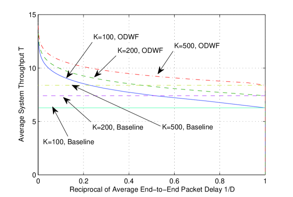
Figure 6: Throughput-delay tradeoff in the fixed relay scenario.

This corollary can be interpreted as follows. If Scheme 1 is implemented, the source just need to guarantee the best $\Theta(1)$ links on each subcarrier are connected links and hence, $\beta=\mathcal{O}(K)$. On the other hand, if Baseline 1 is implemented, one packet can be forwarded to the destination when at least $\Theta(\sqrt{K})$ relays can decode it. Therefore, the source should guarantee the best $\Theta(\sqrt{K})$ links on each subcarrier are connected links, leading to $\beta=\mathcal{O}(\sqrt{K})$. Fig. 6 illustrates the throughput-delay tradeoffs of the ODWF scheme and the baseline scheme for fixed relays according to Theorem 1 and Lemma 3. To normalize the x-axis, we plot the reciprocal of the average end-to-end delay $\frac{1}{D}$ instead. As it’s shown in this figure, the ODWF scheme has the same throughput-delay tradeoff as the baseline scheme in small delay ($D=1$), and achieves larger throughput at the expense of larger delay.

IV Opportunistic decode-wait-and-forward Scheme for Mobile Relays with Macroscopic Fading Channels

In this section, we first describe the proposed opportunistic decode-wait-and-forward relay scheme for mobile relays and macroscopic fading channels, and then discuss its performance. We show that by utilizing buffers in the relays, we could better exploit the mobility of relays and achieve a significantly better performance compared with regular decode and forward relay protocols.

IV-A Relaying Schemes

The proposed ODWF scheme for mobile relays and macroscopic fading channels is described below:

Scheme 2 (ODWF Scheme for Mobile Relays)

• Each relay measures the pathloss to the source and the destination at the channel estimation slot.

• The control slot is divided into two halves, called control sub-slots 1 and 2. The following is the system procedure operating in the control slot:

  • If there exist relays with packets in their buffers and connected link to the destination, a random backoff mechanism is operated in sub-slot 1 to determine which relay could access the destination in the transmission slot.

  • Otherwise, if there exist relays with connected links to the source, these relays will notify the source in sub-slot 2 to transmit a new packet in the transmission slot.

• If one relay is picked up for the transmission slot, this relay will transmit the first packet in its buffer. In the meantime, all other relays should listen and delete from their buffers the same packet. On the other hand, if the source is picked up for the transmission slot, it will broadcast one new packet. Otherwise, no transmission happens in the transmission slots.

In order to demonstrate the performance gain of the ODWF scheme, the existing relay scheme is also presented in the following as a baseline of comparison.

Baseline 2 (Regular Decode-and-Forward Scheme for Mobile Relays)

• Each relay measures the path loss of its links with the source and the destination in the channel estimation slot.

• The control slot is divided into two halves, called control sub-slots 1 and 2:

  • If there is no packet in the relay network, the relays will ask the BS for one new packet in sub-slot 1 (The frame is used for phase I).

  • If there is one packet in the relay network, a cooperative mechanism is performed in sub-slot 2 to determine which relay will forward this packet in the transmission slot (The frame is used for Phase II).

• If one relay is selected in the control slot, this relay will forward the packet to the destination in the transmission slot. Otherwise, if the source is selected in the control slot, it will transmit one new packet to the relay network in the transmission slot.

IV-B Throughput-Delay Tradeoff of ODWF Scheme with Mobile Relays

Since the transmit power is constant, when the source increases the data rate, its radio coverage become small and the number of relays who can decode this packet also becomes small. Hence, the probability these relays can forward the decoded packet to the destination is small, leading to a large end-to-end packet delay. Therefore, there is a tradeoff between the system throughput and the end-to-end packet delay, which is presented rigorously in the following theorem.

Theorem 2 (Throughput-Delay Tradeoff with Mobile Relays)

Denote the data rate as $r=N\log_{2}\beta$. Suppose the Scheme 2 is implemented, for infinite buffers at relays, sufficiently large $K$, and positive $q$:

• The achievable average system throughput of the relay system is upper-bounded by

  $$T_{max}\doteq\frac{N\alpha}{4}\log_{2}K.$$ (10)

  where $\doteq$ denotes the equality with high probability (whp ), and this throughput is achievable under the following conditions:

  $$\lim\limits_{K\rightarrow+\infty}\frac{\ln\beta^{\frac{2}{\alpha}}}{\ln K}=1\quad\mbox{ and }\quad\lim\limits_{K\rightarrow+\infty}\frac{\beta^{\frac{2}{\alpha}}}{K}=0.$$

• If $\lim\limits_{K\rightarrow+\infty}\frac{\beta^{\frac{2}{\alpha}}}{K}=0$, the average system throughput is given by

  $$T\doteq\frac{N}{2}\log_{2}\beta,$$ (11)

  and the average end-to-end packet delay is given by

  $$D\doteq\mathcal{O}\left(\max\{\frac{\beta^{\frac{4}{\alpha}}}{Kq},\frac{1}{q}\}\right).$$ (12)

Proof:

Please refer to Appendix C. ∎

Remarks: (I) Since there are infinitely large buffers at relays and the region transition probability $q$ is positive, the average system throughput is $r/2$ as long as there is always relays having connected links to the source and destination (which is presented mathematically as $\lim\limits_{K\rightarrow+\infty}\frac{\beta^{\frac{2}{\alpha}}}{K}=0$).

(II) There are two factors affecting the average end-to-end delay expression (12), namely $\beta^{\frac{4}{\alpha}}$ and $\frac{1}{q}$. The first factor is related to the packet data rate $r$. When $r$ is large (so as the $\beta$), the source’s coverage becomes small and hence, the number of relays who can decode the packet from the source is small. Therefore, this packet should wait for many frames until these relays carry it into the coverage of the destination. Due to the random walk of the relays’ movement, the less the relays who can decode this packet, the longer time on average this packet should wait. On the other hand, the second factor is relate to the velocity of the relays’ movement. If the velocity is small (so as the region transition probability $q$), statistically one relay should use long time before moving into the coverage of the destination, which also leads to large end-to-end packet delay.

(III) Compared with the throughput of $\mathcal{O}(\ln\ln K)$ in the scenario of fixed relays, exploiting the relays’ mobility could bring the system much larger throughput. Noting that the frame duration is usually milliseconds for the fixed relay scenario but seconds (or even larger) for the mobile relay scenario, the large throughput is obtained at the expense of delay.

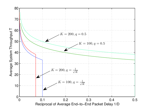
Figure 7: Throughput-delay tradeoff in the mobile relay scenario.

According to Theorem 2, we plot the throughput-delay tradeoff of the ODWF scheme for mobile relays in Fig. 7. To normalize the x-axis, the reciprocal of the average end-to-end delay $\frac{1}{D}$ is plotted instead. As it’s shown in this figure, larger $K$ would lead to larger average system throughput since the system can enjoy more multi-relay diversity. Furthermore, smaller relays’ velocity $q$ would lead to larger average end-to-end packet delay for a given throughput level, having the curve shrink towards the y-axis.

IV-C Comparison with Regular Decode-and-Forward Scheme (Baseline 2)

Before the comparison is made, the performance of the baseline is summarized in the following lemma:

Lemma 2 (Performance of Regular Decode-and-Forward Scheme with Mobile Relays)

For non-zero region-transition-probability $q$ and sufficiently large number of relays $K$, the following statements on the Baseline 2 are true:

• If $\lim\limits_{K\rightarrow+\infty}qK^{\frac{1}{M-1}}<+\infty$, the maximum achievable average system throughput is given by

  $$T_{max}\doteq\mathbf{\Theta}\left(qK^{\frac{1}{M-1}}\right),$$ (13)

  and the corresponding average end-to-end packet delay is $D\doteq\mathbf{\Theta}(\frac{1}{Kq^{M-1}})$.

• If $\lim\limits_{K\rightarrow+\infty}qK^{\frac{1}{M-1}}=\infty$, the maximum achievable average system throughput is given by

  $$T_{max}\doteq\mathbf{\Theta}\left(\log_{2}K\right),$$ (14)

  and the corresponding average end-to-end packet delay is $D\doteq\mathbf{\Theta}(1)$.

Proof:

Please refer to the Appendix D. ∎

Therefore, we have the following corollary on the performance gain of the ODWF scheme:

Corollary 2

Let $T_{o}$ and $T_{r}$ be the optimal average system throughput of the Scheme 2 and Baseline 2, then when $\lim\limits_{K\rightarrow+\infty}qK^{\frac{1}{M-1}}=\infty$,

$$\frac{T_{o}}{T_{r}}=\mathbf{\Theta}(1);$$

and when $\lim\limits_{K\rightarrow+\infty}qK^{\frac{1}{M-1}}<\infty$,

$$\frac{T_{o}}{T_{r}}=\mathbf{\Theta}\left(\frac{\log_{2}K}{qK^{\frac{1}{M-1}}}\right).$$

Although when the relays’ movement is fast ($\lim\limits_{K\rightarrow+\infty}qK^{\frac{1}{M-1}}=\infty$) the average system throughput of the ODWF scheme and the baseline is at the same order, the ODWF could still obtain a gain of constant scaling. This is because the proposed ODWF scheme can exploit the ”idle frame” intelligently before the relays with packets moving into the destination’s coverage. The slower the relays’ movement, the more such ”idle frames” and hence, the larger the throughput gain of the ODWF scheme. Therefore, a orderwise gain can be obtained by ODWF scheme when the relays’ movement is slow, (e.g. $q=\frac{1}{K}$).

V Conclusions

In this paper, we propose an opportunistic decode-wait-and-forward (ODWF) scheme for a point-to-point communication system with $K$ relays. The throughput-delay tradeoff of this ODWF scheme is studied in two scenarios: fixed relays and mobile relays, and the performance gain over the existing relay schemes in the same scenarios is also examined. In the scenario of fixed relays, the ODWF scheme could exploit the spatial and temporal dynamics of multipath fading channels so that it can achieve the same optimal average throughput as the existing schemes with $K^{2}$ relays. In the scenario of mobile relays, the ODWF scheme could exploit the dynamic locations of relays so that the average system throughput can scale as $\Theta(\ln K)$, which can not be achieved by the existing schemes when the relay’s mobility is slow. Moreover, compared with the well-known throughput scaling law of the amplify-and-forward relay networks, where the $\Theta(\log K)$ throughput is achieved with $\Theta(K)$ total transmission power, we show that by exploiting the relays’ mobility the same order of throughput can be achieved even with constant transmission power.

Appendix A: Proof of Theorem 1

We first introduce and prove the following lemma:

Lemma 3

When $\lim\limits_{K\rightarrow+\infty}\frac{\beta}{\sqrt{K}}=+\infty$ and the system has been runing for sufficiently long time, on each subcarrier there are $\alpha\times 100\%$ percentage of relays containing packets in their buffer with high probability, where

$$\alpha=\frac{\ln\left[1-\frac{\delta}{(1+\delta^{N})^{\frac{1}{N}}}\right]}{\ln(1-\delta)}$$

and $\delta=1-(1-\frac{1}{\beta})^{K}$. Moreover, the average system throughput is given by

$$T\doteq\frac{N\delta^{N}}{1+\delta^{N}}\log_{2}[1+p\ln\beta].$$

Proof:

When the source transmits packets to the relay cluster, on each subcarrier there are approximately $e^{-\beta}K$ relays can decode the packet. Hence, the probability that the next frame is used for relay-destination transmission is $\left[1-(1-\frac{1}{\beta})^{\frac{K}{\beta}}\right]^{N}$. Since $\lim\limits_{K\rightarrow+\infty}\frac{\sqrt{K}}{\beta}=0$, we have

$$\lim_{K\rightarrow+\infty}\left[1-(1-\frac{1}{\beta})^{\frac{K}{\beta}}\right]^{N}=0.$$

Thus, those received packets could hardly be forwarded to the destination immediately in the next frame. Instead, they will be stored in the relays’ buffers temporarily. As new packets transmitted from the source become more and more, on every subcarrier the ratio of relays who have packets stored in their buffers become larger and larger. The increase of the ratio will continue until the following flow balance equation is satisfied

$$P_{RD}=P_{SR},$$ (15)

where $P_{SR}$ is the probability one frame is used for source-relay transmission and $P_{RD}$ is the probability one frame is used for relay-destination transmission. Assume the corresponding ratio is $\alpha*100\%$ whp. Since

$$P_{RD}=\left[1-(1-\frac{1}{\beta})^{\alpha K}\right]^{N}$$

and

$$P_{SR} = (1-P_{RD})[1-(1-\frac{1}{\beta})^{K}]^{N},$$

according to(15), we can obtain that

$$\alpha=\frac{\ln\left[1-\frac{\delta}{(1+\delta^{N})^{\frac{1}{N}}}\right]}{\ln(1-\delta)}$$

and

$$P_{SR}=P_{RD}=\frac{\delta^{N}}{1+\delta^{N}},$$ (16)

where $\delta=1-(1-\frac{1}{\beta})^{K}$. As a result, the average throughput is given by

$$T \doteq Nr\times P_{RD}$$

$$\doteq \frac{N\delta^{N}}{1+\delta^{N}}\log_{2}[1+p\ln\beta].$$

where the notation $\doteq$ is necessary due to the randomness of the channel fading.

∎

V-A The proof of statement I:

According to Lemma 3, the achievability is verified below:

$$T \doteq \frac{N\delta^{N}}{1+\delta^{N}}\log_{2}[1+p\ln\beta]$$ (17)

$$\rightarrow \frac{N}{2}\log_{2}[1+p\ln\beta]$$

$$= \frac{N}{2}\log_{2}[1+p\ln K],$$ (18)

where (17) is due to the condition $\lim\limits_{K\rightarrow+\infty}(1-\frac{1}{\beta})^{K}=0$, and (18) is due to $\lim\limits_{K\rightarrow+\infty}\frac{\ln\beta}{\ln K}=1$. In the following, we shall prove that there is no threshold which could lead to a larger average throughput.

It’s easy to see that when $\lim\limits_{K\rightarrow+\infty}\frac{\ln\beta}{\ln K}<1$, the average system throughput $T$ is less than $\frac{N}{2}\log_{2}[1+p\ln K]$. When $\lim\limits_{K\rightarrow+\infty}\frac{\ln\beta}{\ln K}>1$

$$T \doteq \frac{N\delta^{N}}{1+\delta^{N}}\log_{2}[1+p\ln\beta]$$

$$= N\delta^{N}\log_{2}[1+p\ln\beta]$$

$$= N\left[1-(1-\frac{1}{\beta})^{K}\right]^{N}\log_{2}[1+p\ln\beta]$$

$$\rightarrow 0\quad(as\ K\rightarrow+\infty).$$

V-B The proof of the statement II

The proof the this statement is divided into two parts. We shall prove the case when $\lim_{K\rightarrow+\infty}\frac{\beta}{\sqrt{K}}=0$. If the source transmits packets to the relay cluster, on each subcarrier there are approximately $\frac{K}{\beta}$ relays can decode the packet. Hence, the probability that the next frame is used for relay-destination transmission is $\left[1-(1-\frac{K}{\beta})^{\frac{K}{\beta}}\right]^{N}$. Notice that when $\lim_{K\rightarrow+\infty}\frac{\beta}{\sqrt{K}}=0$,

$$\lim_{K\rightarrow+\infty}\left[1-(1-\frac{K}{\beta})^{\frac{K}{\beta}}\right]^{N}=1.$$

The relay-destination transmission will follow the source-relay transmission with probability $1$, thus, the phase I and phase II will occur alternately. Therefore, the average end-to-end packet delay $D$ is $1$ whp and the average system throughput $T$ is $\frac{r}{2}=\frac{N}{2}\log_{2}[1+p\ln\beta]$ whp .

Now we turn to the case when $\lim_{K\rightarrow+\infty}\frac{\beta}{\sqrt{K}}>0$ and $\lim_{K\rightarrow+\infty}\frac{\beta}{K}\leq 1$. The derivation of the average system throughput $T$ can follow the same approach as we did in the proof of statement I. Hence, we only show how to derive the average end-to-end packet delay $D$ in the following.

Suppose the system has been running for sufficiently long time, according to Lemma 3, there are $\alpha\times 100\%$ percent of relays on each subcarrier having packets in the buffers. Notice that $\lim\limits_{K\rightarrow\infty}\alpha=0$, when the source delivers one new packet on each subcarrier, there are $\frac{K}{\beta}$ relays who can decode the packet on each subcarrier, and almost all of them have empty buffer for this subcarrier. Hence, the new arrival packets are on the head of relays’ queues. Notice that $\frac{K}{\beta}<<\alpha K$ and the relay selection if phase II is uniformly random, the probability that one new arrival packet is forward by the relay cluster is given by $P_{RD}\frac{1}{\alpha\beta}$, where $P_{RD}$ is the probability one frame is used for relay-destination transmission which is given by (16). As a result, the average end-to-end packet delay can be written as

$$D \doteq \frac{\alpha\beta}{P_{RD}}$$

$$= 2\alpha\beta$$

$$= 2\beta\frac{\beta}{K}\ln\left(\frac{2^{1/N}}{2^{1/N}-1}\right)$$

$$= \frac{2c\beta^{2}}{K}\quad where\quad c=\ln\left(\frac{2^{1/N}}{2^{1/N}-1}\right),$$

where the second equality is because $P_{RD}\approx\frac{1}{2}$; the third equality is because $\alpha\rightarrow\frac{\beta}{K}\ln\left(\frac{2^{1/N}}{2^{1/N}-1}\right)$ for $K\rightarrow+\infty$ according to Lemma 3. Combine the results in the case of $\lim_{K\rightarrow+\infty}\frac{\beta}{\sqrt{K}}=0$, (8) is proved.

Appendix B: The Proof of Lemma 1

The achievability is verified below. Let $\beta=\sqrt{K}/\ln K$. When the source transmits packets to the relay cluster, there are $\frac{K}{\beta}=\sqrt{K}\ln K$ relays on each subcarrier who can decode the packets. Hence, on every subcarrier, the chance the received packets can be forwarded to the destination in the next frame is $1-\left(1-\frac{1}{\beta}\right)^{\sqrt{K}\ln K}\rightarrow 1$. In other words, packets in the relay cluster can be forward to the destination in the next frame whp , and the average throughput is given by:

$$T \doteq \frac{N}{2}\log_{2}\left[1+p(\ln\sqrt{K}-\ln\ln K)\right]$$ (19)

$$\approx \frac{N}{2}\log_{2}(1+p\ln\sqrt{K}).$$

In the following, we shall continue to show that there is no $\beta$ which can lead to an average throughput larger than $\frac{N}{2}\log_{2}(1+p\ln\sqrt{K})$. Thus, three cases are discussed:

• $\lim\limits_{K\rightarrow+\infty}\frac{\ln\beta}{\ln K}\leq\frac{1}{2}$: It’s obvious that the average throughput in this case can not be larger than $\frac{N}{2}\log_{2}(1+p\ln\sqrt{K})$.

• $\frac{1}{2}<\lim\limits_{K\rightarrow+\infty}\frac{\ln\beta}{\ln K}\leq 1$: After the source’s transmission, there are $\frac{K}{\beta}$ relays on each subcarrier who can decode the packets. Hence, for any packet in the relays’ buffers, it can choose one connected link out of $NK/\beta$ links. Therefore, the probability this packet can be delivered to the destination is upper bounded by $1-\left(1-\frac{1}{\beta}\right)^{NK/\beta}$, and the average throughput is upper bounded by $\left[1-\left(1-\frac{1}{\beta}\right)^{NK/\beta}\right]\frac{r}{2}\rightarrow 0$ (when $K\rightarrow+\infty$).

• $\lim\limits_{K\rightarrow+\infty}\frac{\ln\beta}{\ln K}>1$: It’s with high probability that no relay can decode the packets from the source in this case. Hence, the throughput of this case tends to zero.

In conclusion, the average throughput in (19) is maximum for Scheme 1.

Appendix C: The Proof of Theorem 2

We first prove the second statement, from which the first statement can be deduced.

The Proof of The Statement II - Average System Throughput

Lemma 4

For the threshold $\beta$ satisfying $\lim\limits_{K\rightarrow+\infty}\frac{\beta^{\frac{2}{\alpha}}}{K}=0$ and sufficiently large $K$, the probability that there are $\mathbf{\Theta}(\frac{K}{\beta^{\frac{2}{\alpha}}})$ relays having connected links with the source (or the destination) tends to $1$.

Proof:

Without loss of generality, we only study the number of connected links with the source. The connection with the destination can follow the same approach. It’s equivalent to examine the another relay distribution where the relays’ location on the disk is uniform and i.i.d. between frames.

Since we are interested in the analysis with the sufficiently large $K$ and the monotonically increasing data rate $r$ ($\lim\limits_{K\rightarrow+\infty}r=+\infty$), the coverage radii of the source and the destination in our analysis are sufficiently small given the fixed transmit power $p$. Therefore, for relays with connected links to the source/destination, the link capacity defined in (2) and (3) can be approximated as

$$C^{s,j}\approx N\log_{2}\frac{p}{d_{s,j}^{\alpha}}\quad\mbox{and}\quad C^{j,d}\approx N\log_{2}\frac{p}{d_{j,d}^{\alpha}},$$

and the coverage radius of the source within which the relays have connected links to the source is given by

$$d=\frac{p^{\frac{1}{\alpha}}}{\beta^{\frac{1}{\alpha}}}.$$

Therefore, the area of the source’s coverage can be approximated as $\frac{\pi d^{2}}{2}$, and the probability one relay falls into the source’s coverage is $\frac{d^{2}}{2R^{2}}$.

Suppose there are $X$ relays having connected links with the source, therefore,

$$\Pr(X=x) = \binom{K}{x}\left(\frac{d^{2}}{R^{2}}\right)^{x}\left(1-\frac{d^{2}}{R^{2}}\right)^{K-x}.$$ (20)

From the above equation, the probability that $X=\mathbf{\Theta}(\frac{d^{2}}{R^{2}}K)$ tends to 1 when $K\rightarrow+\infty$. ∎

Notice that there are (with probability $1$) some relays in region $1$ can decode the source’s packets, the relay buffer is infinite, relays are moving among the divided regions, and there are (with probability $1$) some relays in region $M$ can forward packets to the destination, the average system throughput is

$$T\doteq\frac{r}{2}=\frac{N}{2}\log_{2}\beta.$$

The Proof of The Statement II - Average Packet Delay

We study the system in the following two cases: (1) $\lim\limits_{K\rightarrow+\infty}\frac{\beta^{\frac{4}{\alpha}}}{K}=0$, and (2)$\lim\limits_{K\rightarrow+\infty}\frac{\beta^{\frac{4}{\alpha}}}{K}>0$ and $\lim\limits_{K\rightarrow+\infty}\frac{\beta^{\frac{2}{\alpha}}}{K}=0$. The average end-to-end packet delay for the these two cases is given by the following two lemmas.

Lemma 5

For the threshold $\beta$ satisfying $\lim\limits_{K\rightarrow+\infty}\frac{\beta^{\frac{4}{\alpha}}}{K}=0$, the average end-to-end packet delay is given by $D=\mathcal{O}(\frac{1}{q})$

Proof:

When the source broadcasts a packet, there are $\mathbf{\Theta}\left(\frac{K}{\beta^{\frac{2}{\alpha}}}\right)$ relays can decode this packet. Since the region transition probability is $q$, after $\mathbf{\Theta}(1/q)$ frames, there are $\mathbf{\Theta}\left(\frac{K}{\beta^{\frac{2}{\alpha}}}\right)$ relays with this packet moves into the region $M$. Then, this packet can be forwarded to the destination with probability $1$, because

$$\frac{K}{\beta^{\frac{2}{\alpha}}}\frac{1}{\beta^{\frac{2}{\alpha}}}\rightarrow+\infty\mbox{ when }K\rightarrow+\infty.$$ (21)

∎

Lemma 6

For the threshold $\beta$ satisfying $\lim\limits_{K\rightarrow+\infty}\frac{\beta^{\frac{4}{\alpha}}}{K}>0$ and $\lim\limits_{K\rightarrow+\infty}\frac{\beta^{\frac{2}{\alpha}}}{K}=0$, the average end-to-end packet delay is given by $D=\mathcal{O}(\frac{\beta^{\frac{4}{\alpha}}}{Kq})$

Proof:

To prove the average packet delay for the second case is $\mathcal{O}(\frac{\beta^{\frac{4}{\alpha}}}{Kq})$, we first suppose

$$\lim_{K\rightarrow+\infty}\frac{D}{\frac{\beta^{\frac{4}{\alpha}}}{Kq}}=\infty,$$

and then show the contradiction in the following.

Let $D=\frac{\beta^{\frac{4}{\alpha}}}{Kq}\delta$, where $\lim\limits_{K\rightarrow+\infty}\delta=+\infty$. The average packet delay is $D$ implies that the average number of packets stored in the relay network is $\mathbf{\Theta}(D)$. Hence, there are $\mathbf{\Theta}(\frac{\beta^{\frac{4}{\alpha}}}{Kq}\delta)$ packets stored in the relay networks for at least $\mathbf{\Theta}(1/q)$ frames. Therefore, it can be easily seen that there are $\mathbf{\Theta}(\beta^{\frac{2}{\alpha}}\delta)$ relays with packets in region $M$, which implies that the relays will deliver packets to the destination in every frame. Hence, this assumption is impossible. ∎

The Proof of The Statement I

The achievability can be verified by letting $\beta=\left(\frac{K}{\ln^{2}K}\right)^{\frac{\tau}{2}}$. In order to prove the throughput (10) is maximum,two cases are discussed in the following:

• Case I: $\lim\limits_{K\rightarrow+\infty}\frac{\beta}{K^{\frac{\tau}{2}}}=C$ where $C$ is a constant. It’s easy to verify that in this case the average system throughput can not be larger than (10).

• Case II: $\lim\limits_{K\rightarrow+\infty}\frac{\beta}{K^{\frac{\tau}{2}}}=+\infty$. The probability that there is no relay in the source’s coverage is $\left[1-(\frac{p}{\beta})^{\frac{2}{\tau}}\frac{M}{2R^{2}}\right]^{\frac{K}{M}}$, hence the average system throughput is given by

  $$T = \left\{1-\left[1-(\frac{p}{\beta})^{\frac{2}{\tau}}\frac{M}{2R^{2}}\right]^{\frac{K}{M}}\right\}\frac{N}{2}\log_{2}\beta$$

  $$\approx (\frac{p}{\beta})^{\frac{2}{\tau}}\frac{K}{2R^{2}}\frac{N}{2}\log_{2}\beta$$

  $$\rightarrow 0\ \ (as\ \ K\rightarrow+\infty).$$

This completes the proof of Theorem 2.

Appendix D: The Proof of Lemma 2

When the source transmit one packet to the relay network, the probability that there are $\mathbf{\Theta}\left(\frac{K}{\beta^{\frac{2}{\alpha}}}\right)$ relays can decode the packet tends to $1$ (following the same approach as in Appendix C). Then, after $t$ frames, the number of relays who moves into the region 2 from the region 1 is $\mathbf{\Theta}\left(\frac{K}{\beta^{\frac{2}{\alpha}}}qt\right)$; the number of relays who moves into the region 3 from the region 2 from is $\mathbf{\Theta}\left(\frac{K}{\beta^{\frac{2}{\alpha}}}(qt)^{2}\right)$,…, the number of relays who moves into the region M-1 from the region M from is $\mathbf{\Theta}\left(\frac{K}{\beta^{\frac{2}{\alpha}}}(qt)^{M-1}\right)$. In order to deliver the packet to the destination, the average end-to-end packet delay $D$ should satisfy

$$\frac{K}{\beta^{\frac{2}{\alpha}}}(qD)^{M-1}\doteq\mathbf{\Theta}(\beta^{\frac{2}{\alpha}}).$$

Therefore, it can be derived from the above equation that

$$D\doteq\mathbf{\Theta}\left[\max\left\{\frac{1}{q}\left(\frac{\beta^{\frac{4}{\alpha}}}{K}\right)^{\frac{1}{M-1}},1\right\}\right],$$

and the average system throughput is given by

$$T \doteq \frac{N}{2D}\log_{2}\beta$$

$$= \mathbf{\Theta}\left[\min\left\{\frac{Nq}{2}\left(\frac{K}{\beta^{\frac{4}{\alpha}}}\right)^{\frac{1}{M-1}}\log_{2}\beta,\frac{N}{2}\log_{2}\beta\right\}\right].$$

The Proof of The Statement I

When $\lim\limits_{K\rightarrow+\infty}qK^{\frac{1}{M-1}}<+\infty$, the average system throughput becomes

$$T\doteq\mathbf{\Theta}\left(\frac{Nq}{2}\left(\frac{K}{\beta^{\frac{4}{\alpha}}}\right)^{\frac{1}{M-1}}\log_{2}\beta\right).$$

After maximizing with respect to $\beta$ ($\beta=\mathbf{\Theta}(1)$, we have

$$T_{max}\doteq\mathbf{\Theta}\left(\frac{Nq}{2}K^{\frac{1}{M-1}}\right)=\mathbf{\Theta}\left(qK^{\frac{1}{M-1}}\right).$$

The Proof of The Statement II

When $\lim\limits_{K\rightarrow+\infty}qK^{\frac{1}{M-1}}=+\infty$, the optimal $\beta$ which maximizes the average system throughput is

$$\beta^{\frac{4}{\alpha}}=\mathbf{\Theta}(qK^{\frac{1}{M-1}}).$$

Therefore,

$$T\doteq\mathbf{\Theta}\left(\frac{N}{2}\log_{2}q^{\frac{\alpha}{4}}K^{\frac{\alpha}{4(M-1)}}\right)=\mathbf{\Theta}\left(\log_{2}K\right).$$

This finishes the proof of Lemma 2.

Figure 1: Frame sequences for regular decode-and-forward design and opportunistic decode-wait-and-forward design.

Figure 2: System model of the microscopic fading scenario

Figure 3: The illustration of frame structure, where the length of transmission slot is much larger than that of the estimation slot and control slot.

References

- [1] E. van der Meulen, “Transmission of information in a t-terminal discrete memoryless channel,” Ph.D. dissertation, Dep. of Statistics, University of California, Berkeley, 1968.
- [2] ——, “Three-terminal communication channels,” Adv. Appl. Prob., vol. 3, pp. 120–154, 1971.
- [3] ——, “A survey of multi-way channels in information theory: 1961-1976,” Information Theory, IEEE Transactions on, vol. 23, no. 1, pp. 1–37, Jan 1977.
- [4] T. Cover and A. Gamal, “Capacity theorems for the relay channel,” Information Theory, IEEE Transactions on, vol. 25, no. 5, pp. 572–584, Sep 1979.
- [5] A. Gamal and M. Aref, “The capacity of the semideterministic relay channel (corresp.),” Information Theory, IEEE Transactions on, vol. 28, no. 3, pp. 536–536, May 1982.
- [6] Z. Zhang, “Partial converse for a relay channel,” Information Theory, IEEE Transactions on, vol. 34, no. 5, pp. 1106–1110, Sep 1988.
- [7] L.-L. Xie and P. Kumar, “An achievable rate for the multiple-level relay channel,” Information Theory, IEEE Transactions on, vol. 51, no. 4, pp. 1348–1358, April 2005.
- [8] A. Reznik, S. Kulkarni, and S. Verdu, “Broadcast-relay channel: capacity region bounds,” Information Theory, 2005. ISIT 2005. Proceedings. International Symposium on, pp. 820–824, 4-9 Sept. 2005.
- [9] G. Kramer, M. Gastpar, and P. Gupta, “Cooperative strategies and capacity theorems for relay networks,” Information Theory, IEEE Transactions on, vol. 51, no. 9, pp. 3037–3063, Sept. 2005.
- [10] Y. Liang and G. Kramer, “Rate regions for relay broadcast channels,” Information Theory, IEEE Transactions on, vol. 53, no. 10, pp. 3517–3535, Oct. 2007.
- [11] A. Host-Madsen, “A new achievable rate for cooperative diversity based on generalized writing on dirty paper,” Information Theory, 2003. Proceedings. IEEE International Symposium on, pp. 317–317, June-4 July 2003.
- [12] ——, “Capacity bounds for cooperative diversity,” Information Theory, IEEE Transactions on, vol. 52, no. 4, pp. 1522–1544, April 2006.
- [13] P. Gupta and P. Kumar, “The capacity of wireless networks,” Information Theory, IEEE Transactions on, vol. 46, no. 2, pp. 388–404, Mar 2000.
- [14] A. Gamal, J. Mammen, B. Prabhakar, and D. Shah, “Throughput-delay trade-off in wireless networks,” INFOCOM 2004. Twenty-third AnnualJoint Conference of the IEEE Computer and Communications Societies, vol. 1, pp. –475, March 2004.
- [15] S. Toumpis and A. Goldsmith, “Large wireless networks under fading, mobility, and delay constraints,” INFOCOM 2004. Twenty-third AnnualJoint Conference of the IEEE Computer and Communications Societies, vol. 1, pp. –619, March 2004.
- [16] S. Kulkarni and P. Viswanath, “A deterministic approach to throughput scaling in wireless networks,” Information Theory, IEEE Transactions on, vol. 50, no. 6, pp. 1041–1049, June 2004.
- [17] M. Franceschetti, O. Dousse, D. N. C. Tse, and P. Thiran, “Closing the gap in the capacity of wireless networks via percolation theory,” Information Theory, IEEE Transactions on, vol. 53, no. 3, pp. 1009–1018, March 2007.
- [18] S. Aeron and V. Saligrama, “Wireless ad hoc networks: Strategies and scaling laws for the fixed snr regime,” Information Theory, IEEE Transactions on, vol. 53, no. 6, pp. 2044–2059, June 2007.
- [19] A. Ozgur, O. Leveque, and D. Tse, “Hierarchical cooperation achieves optimal capacity scaling in ad hoc networks,” Information Theory, IEEE Transactions on, vol. 53, no. 10, pp. 3549–3572, Oct. 2007.
- [20] M. Grossglauser and D. Tse, “Mobility increases the capacity of ad hoc wireless networks,” Networking, IEEE/ACM Transactions on, vol. 10, no. 4, pp. 477–486, Aug 2002.
- [21] M. Gastpar and M. Vetterli, “On the capacity of wireless networks: the relay case,” INFOCOM 2002. Twenty-First Annual Joint Conference of the IEEE Computer and Communications Societies. Proceedings. IEEE, vol. 3, pp. 1577–1586 vol.3, 2002.
- [22] ——, “On the capacity of large gaussian relay networks,” Information Theory, IEEE Transactions on, vol. 51, no. 3, pp. 765–779, March 2005.
- [23] H. Bolcskei, R. Nabar, O. Oyman, and A. Paulraj, “Capacity scaling laws in mimo relay networks,” Wireless Communications, IEEE Transactions on, vol. 5, no. 6, pp. 1433–1444, June 2006.