Does Unruh radiation accelerate the universe? A novel approach to the cosmic acceleration

Abstract

We present a novel mechanism for the present acceleration of the universe. We find that the temperature of the Unruh radiation perceived by the brane is not equal to the inherent temperature (Hawking temperature at the apparent horizon) of the brane universe in the frame of Dvali-Gabadadze-Porrati (DGP) braneworld model. The Unruh radiation perceived by a dust dominated brane is always warmer than the brane measured by the geometric temperature, which naturally induces an energy flow between bulk and brane based on the most sound thermodynamics principles. Through a thorough investigation to the microscopic mechanism of interaction between bulk Unruh radiation and brane matter, we put forward that an energy influx from bulk Unruh radiation to the dust matter on the brane accelerates the universe.

I Introduction

An unexpected discovery appeared in 1998, that is, our universe is accelerating rather than decelerating acce . This discovery has significant and far-reaching influence on both fundamental physics and astronomy. The invisible sector of the universe (or the modified terms to Einstein gravity) dominates the present evolution and determines the final destiny of the universe. To understand its physical nature, we have to go beyond the standard model. Various explanations of this acceleration have been proposed; see review for recent reviews with fairly complete lists of references of different models. However, the physical nature of the cosmic acceleration remains as a most profound problem in sciences.

In different approaches to the cosmic acceleration problem, braneworld models draw much attention in recent years. Inspired by string/M theory the braneworld gravity is introduced for several problems in standard model, firstly for the hierarchy problem. The braneworld gravity has been extensively studied, for a review, seerev . In the braneworld scenario the standard model particles are confined to a brane, while gravity can propagate in the whole space time. At the low energy region general relativity recovers, while at the high energy region the behavior of gravity is strongly modified. This may yield remarkable changes in gravity dynamics with several different implications for cosmology, black holes and high energy physics. Among various braneworld models, the model proposed by Dvali, Gabadadze and Porrati (DGP) dgpmodel is impressive and a leading one in cosmology. In the DGP model, the bulk is a flat Minkowski spacetime, but a reduced gravity term appears on a tensionless brane. In this model, gravity appears 4-dimensional at short distances but is altered at distance large compared to some freely adjustable crossover scale $r_{0}$ through the slow evaporation of the graviton off our 4-dimensional brane world universe into an unseen, yet large, 5th dimension. At short distances the 4-dimensional curvature scalar $R$ dominates and ensures that gravity looks 4-dimensional. At large distances the 5-dimensional curvature scalar ${}^{(5)}R$ takes over and gravity spreads into extra dimension. The late-time acceleration is driven by the manifestation of the excruciatingly slow leakage of gravity off our four-dimensional world into an extra dimension. This offers an alternative explanation for the current acceleration of the universe dgpcosmology . However, just as LCDM model, it is also suffered from fine-tune problem. In LCDM model, $\Lambda$ is an unimaginatively tiny constant compared to the expectation of the vacuum if our quantum field theory (QFT) is valid till to Planck scale. We know QFT is at least valid at eletro-weak scale, whose expectation of zero-point energy is still $10^{60}$ higher than the scale of the cosmological constant. To solve the dark energy problem in frame of DGP model, people require $r_{c}\sim H_{0}^{-1}$, where $r_{c}$ is a constant, and $H_{0}$ is the present Hubble parameter. Similarly, we can ask why $r_{c}$ is so large that it is approximately equals the Hubble radius.

Interaction is a universal phenomenon in the physics world. An interaction term between bulk and brane has been invoked as a possible mechanism for the cosmic acceleration in frame of braneworld model interbrane . However, in previous works little attention has been devoted to the physical mechanism of such a term. There is a natural physical origin for this interaction which has not been adverted before, that is, Unruh effect. In the braneworld scenario a brane is moving in the bulk, and generally speaking, its proper acceleration does not vanish. Thus, a brane, qua an observer in the bulk space, should perceive the Unruh radiation. The Unruh effect of RS II braneworld is investigated in jenn .

Even for a Minkowski bulk, the brane will sense a thermal bath filled with radiations. If the temperature is different from the inherent temperature of the brane, energy flow will appear based on the most sound principles of thermodynamics. There are several different particles are confined to the brane, which are not in thermal equilibrium. Then, what is the inherent temperature of the brane in the frame of gravity theory? It will be useful to give a brief account of the previous approaches, especially on black hole thermodynamics.

The relation between gravity theory and thermodynamics is an interesting and profound issue. The key quantities bridging the gravity and thermodynamics are temperature and entropy. Temperature of an ordinary system denotes the the average kinetic energy of microscopic motions of a single particle. To gravity the temperature becomes subtle. Since we do not have a complete quantum theory of gravity, for general case we can not use the usual way to get the temperature of the gravity field. Under this situation people set up some thermodynamics and statistical quantities of gravity by using semi-quantum (matter field is quantized, but gravity remains classical) theory, though the concept of gravitational particle is not clear. The black hole thermodynamics (in fact, spacetime thermodynamics, because the physical quantities in black hole thermodynamics should be treated as the quantities of the globally asymptomatic flat manifold) is set up in 4law and confirmed by Hawking radiation hawk .

In the initial work 4law , the temperature of the spacetime is suspected by an analogy to the ordinary thermodynamics. Shortly, it is recognized that the temperature is just the temperature of the radiation emitted from the black hole by a semi-quantum treatment. The method in hawk depends on the global structure of the spacetime. The vacuum state is treated as nonvacuum state by observers at spacelike infinity, which roots in the fact that vacuum state around the black hole is different from the vacuum at spacelike infinity. Along this clue Unruh found that a uniformly accelerating particle detector with proper acceleration $A$ in Minkowski vacuum perceives different excited modes exactly in Bose-Einstein distribution with a temperature $T=A/2\pi$ unruh . Unruh effect helps us to derive the local temperature of a gravitational system. Unruh effect has inherent relations to Hawking effect. After a conformal transformation, the thermal particles detected by an accelerated detector becomes thermal particles seen by an inertial observer in curved spacetime, which is just the Hawking effect in the case of black hole bril .

The laws of black hole mechanics are results of classical Einstein gravity, for qualification of laws of thermal dynamics the quantum theory is required. The mathematical form keeps invariant. This implies that the classical gravity theory may hide information from quantum theory. This possibility is investigated in jaco . The Einstein equation is reproduced from the proportionality of entropy and horizon area together with the first law of thermal dynamics, $\delta Q=TdS$, jointing to heat, entropy, and temperature, where the temperature is the Unruh temperature to an observer just behind a causal Rindler horizon. The entropy is supposed to be proportional to the area of this horizon and the heat flow is measured by this observer. The significance of this derivation is that the Unruh effect is a result of quantum field theory but the derivation of classical Einstein theory depends on it.

More directly, for a dynamical spacetime, a similar procedure reproduces the Friedmann equation. In this case one should apply the first law of thermodynamics to the trapped surface (apparent horizon) of an FRW universe and assume the geometric entropy given by a quarter of the apparent horizon area and the temperature given by the inverse of the apparent horizon cai . There are several arguments that the apparent horizon should be a causal horizon and is associated with the gravitational entropy and Hawking temperature bak . So, for an expanding universe, the Hawking temperature at the apparent horizon should be treated as the inherent temperature of the universe. For a brane universe its inherent temperature may be higher or lower than the temperature of the Unruh radiation in the bulk, which thus triggers an energy flow between brane and bulk. We will study this possibility in frame of DGP braneworld model.

This paper is organized as follows: In the next section we give the basic construction of DGP model and present the Unruh temperature perceived by an inertial observer (inertial respective to the brane, which we will explain in detail) on the brane. In section III, we investigate the condition for the temperature to be valid. In section IV, we study geometric temperature of a DGP brane in detail and find the thermal equilibrium condition for the Unruh radiation and the brane (evaluated by its geometric temperature). In section V, we present a detailed study of the energy exchange between bulk Unruh radiation and the brane matter by statistical mechanics. Our conclusion and discussion appear in section VI.

II Unruh effect for a DGP brane

In this section we discuss the Unruh effect for a DGP brane. Before studying the Unruh effect of a brane, we shall first give a brief review of the gravitational thermodynamics and Unruh effect in 4 dimensional theory, especially the reality of this significant effect.

Unruh effect states that the concept of particle depends on observer. This amazing effect generates some puzzles, sometimes even treated as paradoxes.

First, Unruh’s original construction is not consistent because his quantization is not unitarily equivalent to the standard construction associated with Minkowski vacuum. Hence some authors used mathematically more rigorous methods to solve this problem math .

Second, the temperature of an Unruh particle detector, which is in thermal equilibrium with Unruh radiation it experiences in Minkowski vacuum, is higher than the temperature of the vacuum to an inertial observer. Hence, does it $really$ emit radiation for an inertial observer, just like an accelerated charged particle? It was argued that there was no radiation flux from an Unruh observer no . Unruh made an almost the same calculation as in no , but he found extra terms in the two point correlation function of the field which would contribute to the excitation of a detector 1992 . It was pointed out that the extra terms were missing in no , which shape a polarization cloud about an Unruh detector cloud . The above analysis and detailed analysis (including non-uniformly accelerated observers) in non showed that in a 2-dimensional toy model, there is no radiation flux from the detector. Recently it was found that there exists a positive radiated power of quantum nature emitted by the detector in 4 dimensional space lin .

It should be noted that the response of an Unruh observer to the Minkowski vacuum is independent of its inner structure: The distribution of the different excited modes perceived by the observer depends only on the acceleration of the observer. This implies that the Unruh temperature is an inherent property of the quantum field. The detector only plays the role of test particles. This effect still exists even without a detector, which can be seen clearly from the derivation by Bogolubov transformation. The Unruh effect can be also derived in terms of the spontaneous excitation of accelerating atoms Audretsch94 ; ZYL06 ; ZY07 .

Several contemporary research themes, for example, the black hole thermodynamics wald , the quantum entanglement state yuhan , the Lorentz symmetry breaking kkrs . For extensive references of the Unruh effect, see a recent review article ureview .

Before studying the Unruh effect for a DGP brane we warm up by a short review the DGP brane. The basic construction of DGP model can be written as follows dgpmodel ,

$$S=S_{\rm bulk}+S_{\rm brane},$$ (1)

where

$$S_{\rm bulk}=\int d^{5}x\sqrt{-{}^{(5)}g}\left[{1\over 2\kappa^{2}}{}^{(5)}R\right],$$ (2)

and

$$S_{\rm brane}=\int d^{4}x\sqrt{-g}\left[{1\over\kappa^{2}}K^{\pm}+L_{\rm brane}(g_{\alpha\beta},\psi)\right].$$ (3)

Here $\kappa^{2}$ is the 5-dimensional gravitational constant, ${}^{(5)}R$ is the 5-dimensional scalar curvature. The induced metric $g_{\mu\nu}$ is defined as

$$g_{\mu\nu}={}^{(5)}g_{\mu\nu}+n_{\mu}n_{\nu},$$ (4)

where the lower case of Greeks run from $0\sim 3$, and $n_{\mu}$ is the normal to the brane. $x^{\mu}~{}(\mu=0,1,2,3)$ are the induced 4-dimensional coordinates on the brane, $K^{\pm}$ is the trace of extrinsic curvature on either side of the brane and $L_{\rm brane}(g_{\alpha\beta},\psi)$ is the effective 4-dimensional Lagrangian, which is given by a generic functional of the brane metric $g_{\alpha\beta}$ and matter fields $\psi$ on the brane. In this article we adopt a mostly negative signature. For DGP model, an induced 4 dimensional Ricci scalar term appears in the brane Lagrangian $L_{\rm brane}$,

$$L_{\rm brane}={\mu^{2}\over 2}R+L_{\rm m},$$ (5)

where $\mu$ is the reduced 4 -dimensional Planck mass, $R$ denotes the scalar curvature on the brane, and $L_{\rm m}$ stands for the Lagrangian of matters on the brane.

Assuming a Friedmann-Robertson-Walker (FRW) metric on the brane, we can derive the Friedmann equation on the brane dgpcosmology (for a more extensive study of the DGP cosmology in which a Gauss-Bonnet term a Weyl term appear in the bulk, see gbzhang ),

$$H^{2}+\frac{k}{a^{2}}=\frac{\rho}{3\mu^{2}}+\frac{2}{r_{c}^{2}}+\frac{2\epsilon}{r_{c}}\left(\frac{\rho}{3\mu^{2}}+\frac{1}{r_{c}^{2}}\right)^{1/2},$$ (6)

where $\rho$ denotes matter energy density on the brane, $r_{c}=\kappa^{2}\mu^{2}$, denotes the cross radius of DGP brane, $\epsilon=\pm 1$, represents the two branches of DGP model, $H$ is Hubble parameter, $k$ is spatial curvature, and $a$ is the scale factor of the brane. The branch $\epsilon=1$ was treated as an unstable branch based on the linear order perturbations. However, a recent study shows that ghosts do not appear under small fluctuations of an empty background, and conformal sources do not yield instabilities either stable .

Now we begin to investigate the Unruh effect for a DGP brane in a Minkowski bulk. We work in a bulk-based coordinate system,

$$dS^{2}=d\hat{T}^{2}-dR^{2}-R^{2}d\Omega_{3}^{2},$$ (7)

where $dS^{2}$ is the 5 dimensional line-element, $d\Omega_{3}^{2}$ denotes a 3 dimensional sphere. A free falling observer on the brane, which is just the comoving observer in the FRW universe, can be described in the FRW coordinates,

$$x^{\mu}=(t,x^{1}_{0},x^{2}_{0},x^{3}_{0}),$$ (8)

where $t=x_{0}$ is the standard world time function, and $x^{1}_{0},x^{2}_{0},x^{3}_{0}$ are three coordinates of the unit 3-sphere $\Omega_{3}$. For a comoving observer, they are constants. Hence, clearly its acceleration is zero in the brane-viewpoint. However, it accelerates in the cross direction of the brane, or the direction of extradimension. The observer moves along a non-geodesic orbit measured by the full 5-dimensional metric. This is the exact meaning of “A brane accelerates in the bulk”, and the acceleration of the brane indicates the acceleration of such comoving observers.

We assume a free-falling particle on the brane, as a particle detector, moves along the worldline

$$x^{B}(t)=(\hat{T},R,x^{1}_{0},x^{2}_{0},x^{3}_{0}),$$ (9)

where the capital Latin letters run from $0\sim 4$. For a moving brane in the $R$ direction, the velocity of a free falling observer on the brane reads

$$U^{A}=(\dot{\hat{T}},\dot{R},0,0,0),$$ (10)

which satisfies the normalization condition,

$$U_{A}U^{A}=1.$$ (11)

The induced metric on the brane reads,

$${ds}^{2}=dS^{2}-U\otimes U=dt^{2}-a(t)^{2}d\Omega_{3}^{2},$$ (12)

where we have labeled the radius coordinate $R$ by a new symbol $a$, which is more frequently used in cosmology.

The unit normal of the brane is vertical to the velocity and spacelike,

$$n_{A}U^{A}=0,~{}n_{A}n^{A}=-1.$$ (13)

The acceleration of the brane is defined as,

$$A^{C}=U^{B}\nabla_{B}U^{C}.$$ (14)

We consider the component of the extrinsic curvature along the velocity,

$$K_{tt}=K_{AB}U^{A}U^{B}=-n_{C}A^{C}.$$ (15)

By using the junction condition across the brane

$$[K_{\mu\nu}]=-\kappa^{2}(s_{\mu\nu}-\frac{1}{3}g_{\mu\nu}s),$$ (16)

where $[K_{\mu\nu}]$ denotes the difference of the extrinsic curvatures of the two sides of the brane, $s_{\mu\nu}$ represents the energy-momentum confined to the brane, we derive the amplitude of the acceleration of brane lang ,

$$A=\left|{}^{(5)}g_{CD}A^{C}A^{D}\right|^{1/2}=\frac{\kappa^{2}}{6}\left|2\rho_{e}+3p_{e}\right|.$$ (17)

Here $\rho_{e}$ and $p_{e}$ are the effective energy density and pressure of the brane, which are defined as

$$\rho_{e}=s_{0}^{0},$$ (18)

$$p_{e}=-s_{i}^{i},$$ (19)

where $i$ is an arbitrary spatial index and we need not sum over the index $i$. And $s$ is the effective energy momentum confined to the brane,

$$s_{\mu\nu}\triangleq\frac{2}{\sqrt{-g}}\frac{\delta({\sqrt{-g}L_{\rm brane}})}{\delta g_{\mu\nu}},$$ (20)

where $L_{\rm brane}$ is given by (5). Due to the above equation, the energy momentum $s_{\mu\nu}$ includes the contribution of the matter term $L_{m}$, as well as the induced curvature term $R$ on the brane. That is the reason why we call the density and pressure in (18) and (19) effective density and pressure. We stress that the effective density $\rho_{e}$ is different from the local density $\rho$ of the matter confined to the brane in (6), which does not include the geometric effect of the induced Ricci term $R$.

We see that, generally speaking, $A$ does not vanish. So the brane may perceive Unruh-type radiation in the bulk. To discuss Unruh radiations seen by the observer on the brane, we introduce a 5-dimensional scalar field in the bulk, which is in its Minkowski vacuum state,

$${\cal L}_{\phi}=\frac{1}{2}\partial_{A}\phi\partial^{A}\phi-\frac{1}{2}m^{2}\phi^{2},$$ (21)

where $m$ denotes $\phi$’s mass parameter. Since the scalar is in its vacuum state, classically it does no work on the brane and bulk dynamics.

Several different methods have been proposed to derive Unruh effect since Unruh’s original work bril . Here we use the Green function method. We consider a detector minimally coupled to a 5-dimensional scalar field $\phi$ in the bulk .

The Lagrangian $cm(t)\phi[x(t)]$ describes the interaction between detector and field, where $c$ is the coupling constant and $m$ denotes the moment operator of the detector. It is shown in bril that, for a small number $c$, the probability amplitude of the transition from the ground state $|E_{0}>$ of a particle detector coupled to a scalar field in its vacuum state $|0_{M}>$ to an excited state $|E>$, where $M$ stands for Minkowski, reads

$$c^{2}\sum_{E}|<E|m|0_{M},E_{0}>|^{2}{\cal F}(E-E_{0}),$$ (22)

where the detector response function ${\cal F}(E)$ is defined as

$${\cal F}(E-E_{0})=\int^{\infty}_{-\infty}dt\int^{\infty}_{-\infty}dt^{\prime}G^{+}(x(t),x(t^{\prime}))e^{-i(E-E_{0})(t-t^{\prime})},$$ (23)

and the Wightman Green function $G^{+}(x,x^{\prime})$ is defined as

$$G^{+}=<0_{M}|\phi(x)\phi(x^{\prime})|0_{M}>.$$ (24)

We note that the term $|<E|m|0_{M},E_{0}>|^{2}$ depends on the structure of the particle detector, but ${\cal F}(E-E_{0})$ does not, which reflects the inherent properties of quantum fields. It is clear that for a general trajectory the response function is not zero.

For a uniformly accelerated trajectory the Wightman Green function becomes a function of $\Delta t=t-t^{\prime}$. Since the detector will detect infinite particles in its whole history, the response function (23) is not well-defined. Under this situation it will make sense to consider the unit response function, which describes in unit time interval,

$${\cal U}(E-E_{0})=\int^{\infty}_{-\infty}d\Delta te^{-i(E-E_{0})\Delta t}G^{+}(\Delta t).$$ (25)

Since $x_{0}^{1},x_{0}^{2},x_{0}^{3}$ are constant, we just set $x_{0}^{1}=x_{0}^{2}=x_{0}^{3}=0$ after a coordinates transformation. For a uniformly accelerated observer in the cross-brane direction, the coordinates in (9) read,

$$x_{0}^{1}=x_{0}^{2}=x_{0}^{3}=0,~{}\hat{T}=\frac{\sinh(tA)}{A},R=\frac{\cosh(tA)}{A},$$ (26)

where $A$ is a constant, denoting the magnitude of acceleration of the detector. Then, integrating (24) directly with proper boundary condition (corresponding to proper contour bril ), we obtain its concrete form in McDonald function (Bessel function with imaginary arguments),

$$G^{+}(\Delta t)=\frac{e^{i5\pi/4}(mA)^{3/2}}{16\pi^{5/2}(\sinh(A\Delta t/2-i\varepsilon))^{3/2}}K_{3/2}\left(\frac{i2m}{A}\sinh(A\Delta t/2-i\varepsilon)\right),$$ (27)

where, as usual, $\varepsilon$ is a small positive number. The Wightman Green function for massless mode reads,

$$D^{+}({\Delta t})=\lim_{m\to 0}G^{+}(\Delta t)=-\frac{i}{64\pi^{2}}\frac{A^{3}}{(\sinh(A\Delta t/2-i\varepsilon))^{3}}.$$ (28)

Generally speaking, Unruh effect is a very weak effect. For example, in 4 dimensional Minkowski space, it needs about an acceleration $10^{21}$ meter per second² to increase temperature 1 K, hence various massive modes are difficult to be excited. The mode with zero mass is the easiest mode to be excited. Therefore, we consider excitations of massless modes. Substituting $D^{+}({\Delta t})$ into (25), one obtains the unit response function with a contour closed at lower half plane of complex $\Delta t$ by using the Jordan’s lemma,

$${\cal U}(E-E_{0})=\frac{1}{32\sqrt{\pi}}\frac{A^{2}+4(E-E_{0})^{2}}{e^{2\pi(E-E_{0})/A}+1}.$$ (29)

This is the response function for a particle detector confined to the FRW brane, and comoving to the FRW brane, which describes photon gas system at temperature $A/2\pi$. We see that a Fermi-Dirac factor appears, which implies that the particles of Rindler radiation behaves as Fermions, though all the excited modes we integrated to derive the response function are Bosonic. It is not a phenomenon completely new. In 1986, Unruh pointed out that the Fermi-Dirac factor would appear in the response function for an accelerated monopole of a massless field in an odd number of space dimension, arising from integration over all modes for a scalar field unruh .

In the above text of this section, only a brane with positive spatial curvature is discussed. A spatially flat brane can be treated as a limit when $R$ is large enough. To the case of a negative spatial curvature, we need to replace the 3-sphere by a 3-hyperbola $H_{3}$ in (7). A 5-dimensional Minkowski space sliced with space-like 3-hyperbola can be written as,

$$dS^{2}=-d\hat{T}^{2}+dR^{2}-R^{2}dH_{3}^{2}.$$ (30)

Then the following discussions exactly follow the case of positive spatial curvature. The resulting distribution function (29) is still valid.

III Quasi-stationary acceleration stage

Up to now our analysis is limited to uniformly accelerated detectors. But from (17) we see that the acceleration of the brane is not a constant. Physically, the formula (29) remains valid when the acceleration varies slowly. Mathematically we can estimate the time over which the constant acceleration approximation is valid by imposing that the variations in the acceleration are small, e.g., expanding the acceleration around some time $t_{0}$ to the first order $t-t_{0}$:

$$A(t)=A(t_{0})+(t-t_{0})\frac{dA}{dt}\left|{}_{t=t_{0}}\right.$$ (31)

Here, we adopt the cosmic time (proper time) $t$ rather than the proper time coordinate time $\hat{T}$ of the detector since the cosmic time is directly related to our measurement of cosmological parameters. For evaluating the variation of the acceleration, define characteristic time

$$t_{c}\triangleq\left|\frac{A(t_{0})}{dA/dt|_{t=t_{0}}}\right|,$$ (32)

which is a function of $t_{0}$, i.e., it varies with the evolution of the universe. Our condition for “acceleration varies slowly” requires that the time scale of a physical process we concerned is much less than the characteristic time,

$$t_{i}\ll t_{c}.$$ (33)

The time scale of a physical process $t_{i}$ must be shorter than the age of the universe. So if the characteristic time $t_{c}$ is much larger than the time scale of the universe, we can safely treat the acceleration as a constant for any physical processes.

Here we present some examples to explain this condition. We work in a frame of “$r_{c}$CDM” model, that is, a DGP brane universe filled with dust, whose density function $\rho$ in Friedmann equation (6) only includes pressureless matter, with about $30\%$ of the critical density.

First, we consider the inflationary phase at the early universe. At such a high energy scale, the infrared correction of DGP model to the standard general relativity, which becomes important at late time universe, can be omitted safely. So the effective energy density and pressure in (17) are just the ordinary density and pressure of the universe. At the whole inflationary phase, the density of the universe is approximately constant, and the pressure $p=-\rho$. Hence,

$$\frac{dA}{dt}=-\frac{\kappa^{2}}{6}\frac{d\rho}{dt}\sim 0,$$ (34)

that is, from (32), the characteristic time is very long. In this case, the Unruh temperature is well defined.

Second, the universe enters a radiation dominated phase after the inflation. At this stage, the DGP-correction to the standard model is still tiny. Thus, we adopt the the same approximation as above, $\rho_{e}=\rho,~{}p_{e}=p$. For a radiation dominated universe, we have

$$p=\frac{1}{3}\rho.$$ (35)

The continuity equation reads,

$$\frac{d\rho}{dt}+3H(\rho+p)=0.$$ (36)

Substitute (35) and (36) into (32), we reach,

$$t_{c}=\frac{\sqrt{3}}{4}\frac{\mu}{\sqrt{\rho}},$$ (37)

from which we see that the characteristic time becomes longer when the energy density becomes lower. For instance, when $\rho=(0.1$Mev)⁴, we get $t_{c}\sim 1$s, which is much shorter than the age of the universe at that time.

And then the universe is diluted to be thinner and thinner. The DGP correction becomes more and more important. Under this situation we have to introduce the correction terms. By using (20) (see also eff ), we derive

$$\rho_{e}=\rho-\mu^{2}(3X),$$ (38)

$$p_{e}=p+\mu^{2}(\frac{2\ddot{a}}{a}+X),$$ (39)

where $X$ is defined as

$$X\triangleq H^{2}+k/a^{2}.$$ (40)

Substituting to the Friedmann equation (6), we obtain

$$X=\frac{\rho}{3\mu^{2}}+\frac{2}{r_{c}^{2}}+\frac{2\epsilon}{r_{c}}\left(\frac{\rho}{3\mu^{2}}+\frac{1}{r_{c}^{2}}\right)^{1/2}.$$ (41)

As for standard cosmology, $\frac{2\ddot{a}}{a}$ can be obtained from the Friedmann equation and the continuity equation . Here, similarly, from Friedmann equation (6) and the continuity equation (75), we derive

$$\frac{\ddot{a}}{a}=X-\frac{1}{2\mu^{2}}\frac{\rho+p}{1+\frac{\epsilon}{\sqrt{X}}\frac{1}{r_{c}}}.$$ (42)

Then substituting (38) , (39) and (17) into (32) , we arrive at the following rather complicated from,

$$t_{c}=\frac{1}{3}\left[2+\frac{3\mu^{2}X}{\rho}-{3}{(1+\frac{\epsilon}{r_{c}\sqrt{X}})^{-1}}\right](X-\frac{k}{a^{2}})^{-1/2}V^{-1},$$ (43)

where

$$V=3-\frac{1}{3}(1+\frac{\epsilon}{r_{c}\sqrt{X}})^{-1}+\frac{\epsilon}{r_{c}}\left(\frac{\rho}{3\mu^{2}}+\frac{1}{r_{c}^{2}}\right)^{-1/2}-\frac{1}{2}\frac{\rho}{r_{c}^{2}\mu^{2}X^{3/2}}\left[1+\frac{\epsilon}{r_{c}}\left(\frac{\rho}{3\mu^{2}}+\frac{1}{r_{c}^{2}}\right)^{-1/2}\right].$$ (44)

Substituting the current parameter of the universe $\rho=(1.8\times 10^{-3}$ev$)^{4}$ and we suppose that the universe is spatially flat, then we obtain, either for the negative or the positive branch, $t_{c}\sim 10^{17}$s, which is at the same scale of the age of the universe. So the constant acceleration is a perfect approximation under this condition.

Then, at least of late time universe, we can safely use (29), which is a thermal distribution at a temperature of

$$T=\frac{A}{2\pi}.$$ (45)

Associating with (17), we get

$$T=\frac{\kappa^{2}}{12\pi}|2\rho_{e}+3p_{e}|.$$ (46)

IV compared to geometric temperature of the brane

We see that the temperature of Unruh radiation the brane perceives, as displayed in (46), only relates to the energy density and pressure of the brane for a given DGP model. Then, a natural question emerges: Is the Unruh radiation hotter, colder or at the same temperature to the brane? If there is energy exchange between bulk and brane, we also need the temperature of the brane to decide the direction of the energy flux. But there are several different particles on the brane. They had gone out of thermal equilibrium long before. Hence we’d better to find the characteristic temperature of the braneworld independent of its detailed microscopic construction. As we have pointed out Unruh radiation is a geometric feature of the space, which is unrelated to the construction of the detector. Just as well we need the characteristic temperature of the brane.

We know that the formulae of black hole entropy and temperature have a certain universality in the sense that the horizon area and surface gravity are purely geometric quantities determined by the space geometry, once Einstein equation determines the space geometry. As we have mentioned above, Einstein equation can be reproduced by thermal dynamics considerations. As for the case of cosmology, applying the first law of thermodynamics to the apparent horizon of an FRW universe and assuming the geometric entropy given by a quarter of the apparent horizon area and the temperature given by the inverse of the apparent horizon, the Friedmann equation can be derived. This celebrated result implies that the inverse number of the apparent horizon is the geometric temperature of the universe, which is independent of the microscopic structures of the particles confined to the brane. The apparent horizon in the dynamical universe is a marginally trapped surface with vanishing expansion. Straightforward calculation yields the radius of the apparent horizon

$$R_{A}=X^{-1/2},$$ (47)

where $X$ is defined in (40). And then the geometric temperature of the brane reads

$$T^{\prime}=\frac{R_{A}^{-1}}{2\pi}=\frac{X^{1/2}}{2\pi}=\frac{1}{2\pi}\sqrt{\frac{\rho}{3\mu^{2}}+\frac{2}{r_{c}^{2}}+\frac{2\epsilon}{r_{c}}\left(\frac{\rho}{3\mu^{2}}+\frac{1}{r_{c}^{2}}\right)^{1/2}}~{}~{}.$$ (48)

Substituting (42) into (39) and (39) and (38) into (46), we arrive at

$$T=\left|\frac{r_{c}}{12\pi\mu^{2}}\left(2\rho+3p\right)+\frac{r_{c}}{4\pi}\left(X-\frac{1}{\mu^{2}}\frac{\rho+p}{1+\frac{\epsilon}{\sqrt{X}}\frac{1}{r_{c}}}\right)\right|,$$ (49)

where $X$ is given by (41). Therefore we obtain the explicit form temperature of the brane, which is determined by its energy density and pressure. By contrast the geometric temperature only depends on the energy density, which has no relation to the pressure. We see that both Unruh temperature (49) and geometric temperature (48) are unrelated to the spatial curvature of the brane.

To investigate further the evolution of the Unruh temperature and the geometric temperature during the history of the universe, we write them in dimensionless form,

$$\frac{T^{\prime}}{H_{0}}=\frac{X^{1/2}}{2\pi H_{0}}=\frac{1}{2\pi}\left[x\Omega_{m}+2\Omega_{r_{c}}+2\epsilon\sqrt{\Omega_{r_{c}}}(x\Omega_{m}+\Omega_{r_{c}})^{1/2}\right]^{1/2},$$ (50)

$$\frac{T}{H_{0}}=\frac{A}{2\pi H_{0}} = \left|\frac{x\Omega_{m}}{2\pi\sqrt{\Omega_{r_{c}}}}(1+3w/2)+\frac{1}{4\pi\sqrt{\Omega_{r_{c}}}}\left[\frac{X}{H_{0}^{2}}-3\Omega_{m}x(1+w)\frac{1}{1+\frac{\epsilon}{\sqrt{X/H_{0}^{2}}}\sqrt{\Omega_{r_{c}}}}\right]\right|,$$ (51)

$$= \left|\frac{x\Omega_{m}}{2\pi\sqrt{\Omega_{r_{c}}}}(1+3w/2)+\frac{1}{4\pi\sqrt{\Omega_{r_{c}}}}\left[\frac{4\pi^{2}T^{\prime 2}}{H_{0}^{2}}-3\Omega_{m}x(1+w)\frac{1}{1+\frac{\epsilon}{\sqrt{T^{\prime}/H_{0}}}\sqrt{\Omega_{r_{c}}}}\right]\right|$$

where $H_{0}$ is the present value of the Hubble parameter, $w$ is the parameter of state equation of the matter confined to the brane, $x\triangleq\rho/\rho_{0}$, and $\Omega_{m},~{}\Omega_{r_{c}}$ are defined as

$$\Omega_{m}=\frac{\rho_{0}}{3\mu^{2}H_{0}^{2}},$$ (52)

$$\Omega_{r_{c}}=\frac{1}{r_{c}^{2}H_{0}^{2}}.~{}~{}$$ (53)

Here $\rho_{0}$ denotes the present density. First, we study various limits of the two types of the temperatures. When $r_{c}\to\infty,~{}\Omega_{r_{c}}\rightarrow 0$, we expect that DGP brane theory reduces to standard 4-dimensional cosmology. It is right in the case for geometric temperature of the brane,

$$\lim_{r_{c}\to\infty}T^{\prime}=\frac{\sqrt{\rho}}{2\pi\sqrt{3}\mu}.$$ (54)

But for Unruh temperature, it is a different situation. Though all dynamical effect of the 5th dimension vanishes when $r_{c}\to\infty$, the Unruh temperature does not vanish. One can check

$$\lim_{r_{c}\to\infty}T=\frac{1}{2}\left|5+3w\right|\frac{\sqrt{\rho}}{2\pi\sqrt{3}\mu}.$$ (55)

This result implies that even when the gravitational effect of the extra dimension vanishes, the quantum effect is saved. The other important limit is the limit when the matter on the brane is infinitely diluted, i.e., $\rho\to 0$,

$$\lim_{\rho\to 0}T^{\prime}=\frac{\sqrt{2}}{2\pi}\frac{\sqrt{1+\epsilon}}{r_{c}},$$ (56)

$$\lim_{\rho\to 0}T=\frac{1}{2\pi}\frac{1+\epsilon}{r_{c}}.~{}~{}~{}~{}$$ (57)

One may conclude

$$\lim_{\rho\to 0}T^{\prime}=\lim_{\rho\to 0}T,$$ (58)

for either $\epsilon=1$ or $\epsilon=-1$. However

$$\lim_{\rho\to 0}\frac{T^{\prime}}{T}=1,$$ (59)

for $\epsilon=1$, and

$$\lim_{\rho\to 0}\frac{T^{\prime}}{T}=\frac{1}{|2+3w|},$$ (60)

for $\epsilon=-1$, since the “speeds” are different when $T$ and $T^{\prime}$ go to zero.

An important case for cosmology is a universe filled with dust matter, i.e., $w=0$. In this case, (48) and (49) become,

$$T^{\prime}=Z+\epsilon Y,$$ (61)

and

$$T=\left|Y+\epsilon Z+\frac{3}{2}\frac{Z^{2}-Y^{2}}{2Y+\epsilon Z}\right|,$$ (62)

where we set

$$Y=\frac{1}{2\pi}H_{0}\sqrt{\Omega_{r_{c}}}~{},$$ (63)

and

$$Z=\frac{1}{2\pi}H_{0}\sqrt{\Omega_{r_{c}}+x\Omega_{m}}~{}.$$ (64)

For a reasonable cosmological model, we have $Y>0,~{}Z>0$ and $Z>Y$. The calculation to take absolute value is difficult to deal with. Hence we consider different cases in which we can determine the sign in the absolute calculation.

First, in the branch $\epsilon=1$, $T$ becomes

$$T=Y+Z+\frac{3}{2}\frac{Z^{2}-Y^{2}}{2Y+Z},$$ (65)

because every term is larger than zero. Then

$$T-T^{\prime}=\frac{3}{2}\frac{Z^{2}-Y^{2}}{2Y+Z}>0.$$ (66)

Therefore, the Unruh radiation perceived by a brane is warmer than the brane measured by the geometric temperature.

Second, we consider the branch $\epsilon=-1$. The Unruh temperature in this case is much more complicated. First, at the point $2Y=Z$, or equally $3\Omega_{r_{c}}=x\Omega_{m}$, there is a singularity $T\to\infty$ in (62), which means the particle numbers are equal at every energy level. This is valid only for a system endowed with finite energy levels, which indicates our theory must be cut off at some energy level. On the right hand of this singularity $2Y-Z>0$, $T$ can be decomposed in the form

$$T=\left|\frac{(Y-Z)(Y-5Z)}{2(2Y-Z)}\right|,$$ (67)

where $Y-Z<0$, $Y-5Z<0$ and $2Y-Z>0$, hence $\frac{(Y-Z)(Y-5Z)}{2(2Y-Z)}>0$. So we remove the absolute sign directly and compare $T$ and $T^{\prime}$ by

$$T-T^{\prime}=\frac{(Y-Z)(5Y-7Z)}{2(2Y-Z)}>0,$$ (68)

since $Y-Z<0$, $5Y-7Z<0$ and $2Y-Z>0$. On the left hand of this singularity $2Y-Z<0$, similar to the case $2Y-Z>0$, we can prove $\frac{(Y-Z)(Y-5Z)}{2(2Y-Z)}<0$. Hence we remove the absolute sign by inserting a minus sign and, $T-T^{\prime}$ becomes

$$T-T^{\prime}=-\frac{3}{2}\frac{Z^{2}-Y^{2}}{2Y-Z}>0.$$ (69)

Thus we prove that the Unruh radiation perceived by a dust dominated brane is warmer than the brane measured by the geometric temperature all the time.

The other point deserving to be noted is that $T^{\prime}$ will be always equal to $T$ if the parameter of state equation of the matter is confined to brane $w=-1$. In this case,

$$T=T^{\prime}=\frac{1}{2\pi}\left(\epsilon\frac{1}{r_{c}}+\sqrt{\frac{1}{r_{c}^{2}}+\frac{\rho}{3\mu^{2}}}\right).$$ (70)

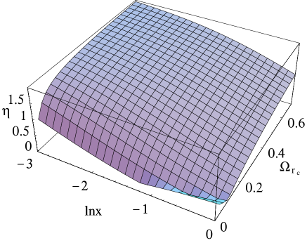
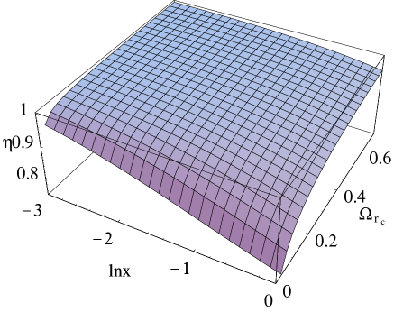
Figure 1: $\eta\triangleq T^{\prime}/T$ as a function of $x$ and $\Omega_{r_{c}}$. In this figure we consider quintessence-like matter dominated universe, in which $w=-1/2$ and we set $\Omega_{m}=0.3$. (a) The branch $\epsilon=-1$. (b) The branch $\epsilon=+1$.

Figure 2: $u\triangleq 2\pi T/H_{0}$ as a function of $v\triangleq 2\pi T^{\prime}/H_{0}$. In this figure we also consider quintessence-like, in which $w=-1/2$ and we set $\Omega_{m}=0.3$. (a) The branch $\epsilon=1$. (b) The branch $\epsilon=-1$.

For general case the expressions of $T$ and $T^{\prime}$ are rather complicated. Hence we plot two figures to give their visual profiles. Fig. 1 illustrates $T^{\prime}/T$ as a function of $x$ and $\Omega_{r_{c}}$. As we have pointed out, when $\rho\to 0$, $T^{\prime}/T\to 1$ for the branch $\epsilon=1$; while when $\rho\to 0$, $T^{\prime}/T\to 1/|2+3w|=1/2$ for the branch $\epsilon=1$. Fig. 2 directly displays $T$ as a function of $T^{\prime}$, in which the interval of the argument $x$ is $x\in(0,3)$. Recalling $x=\rho/\rho_{0}$, we see that we consider the temperatures in some low redshift region and in the future in figure 2. It is clear that $T\to 0$ when $T^{\prime}\to 0$, as shown by (56) and (57) for the branch $\epsilon=1$. Our numerical result also shows an interesting property of the branch $\epsilon=-1$: $T$ is almost a linear function of $T^{\prime}$.

V Unruh radiation accelerates the universe

With the detailed studies in the last sections, we see that the Unruh temperature does not vanish even at the limit $r_{c}\to\infty$, which is the condition for the vanishing of the gravitational effect of the 5th dimension. Furthermore, the Unruh temperature is always higher than geometric temperature for a dust dominated brane in the whole history of the universe for both of the two branches and for all three types of spatial curvature. So an influx from bulk to brane will appear if brane interacts with bulk based on the most sound principle of thermodynamics.

Although this difference in temperature indicates an energy flux, it offers no hint of the form of the interaction term. Under this situation, we explore the microscopic mechanism based on statistical mechanics and particle physics to derive the interaction term between Unruh radiation and dark matter confined to the brane.

In section II, we have considered a detector coupling to a scalar field $L_{\phi}=\frac{1}{2}\partial_{A}\phi\partial^{A}\phi-\frac{1}{2}m^{2}\phi^{2}$, which satisfies 5 dimensional Klein-Gordon equation. At the massless limit, it obeys

$$\square^{(5)}\phi=0.$$ (71)

By using Green function method, we derive the temperature of the Unruh radiation,

$$T=\frac{A}{2\pi},$$ (72)

where $A$ is given by (17).

To investigate the microscopic mechanism of interaction between brane and bulk, one should decompose the 5-dimensional modes, which satisfies (71), into modes along the brane and modes transverse to the brane. Following yling , we call them type I modes and type II modes, respectively. In a pseudo-Euclidean coordinates system, type I mode reads, $\phi^{(I)}=e^{-ik_{\mu}x^{\mu}}$, where $k_{\mu}$ denotes the momentum of the mode in different directions, and $\mu=0,1,2,3$. Type II modes reads, $\phi^{(II)}=e^{-ik_{\mu}x^{\mu}-ik_{y}y}$, where $y$ is the coordinate of the extra dimension, and we require $k_{y}\neq 0$. An arbitrary 5 dimensional mode must be either type I or type II. It was shown in yling that Type II modes of the bulk fluctuations do not interact with the brane, for which the brane is effectively a mirror. Hence only type I mode can exchange energy with matter confined to the brane. We show a schematic plan of type I and type II modes in Fig. 3.

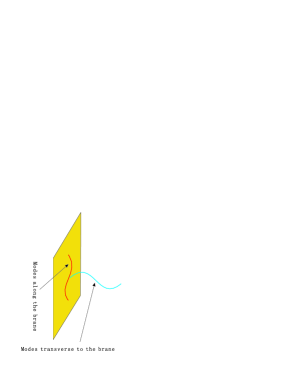
Figure 3: A sketch of type I and type II modes. Only type I mode can exchange energy with particles confined to the brane, while the brane behaves as a perfect mirror for type II mode (for a color version on line).

By a standard process of canonical quantization, type I modes become photons on the brane. Here photons mean quanta without mass, which do not necessarily satisfy Maxwell equations. In fact we do not even need to study its commutativity in detail. Whether they obey Fermi-Dirac statistics or Bose-Einstein statistics the number density of the photon gas $n_{\gamma}$ is proportional to the cubic of its temperature,

$$n_{\gamma}\propto T_{\gamma}^{3},$$ (73)

where $T_{\gamma}$ is just the temperature of the Unruh radiation (45). The particles confined to the brane are immerged in the thermal bath of these photons. Therefore, based on statistical mechanics the reaction rate $\Gamma$ between dark matter particles and the type I photons is proportional to the number densities of photons and dark matter particles, the relative velocity of the photons and matter particles, and the scattering cross section $\Gamma\propto n_{\rm dm}n_{\gamma}\sigma v_{\rm pm}$. Here, $n_{\rm dm}$ denotes the number density of dark matter particle, $v_{\rm pm}$ stands for the relative velocity, which is a constant, and $\sigma$ represents the scattering cross section. In a low energy region, the internal freedoms can not be excited. This paper concentrates on the late time universe, hence the cross section is effectively constant. Therefore, the reaction rate can be written as an equation by inserting a constant $b$,

$$\Gamma=b\rho A^{3},$$ (74)

where we have used (73), (45) and $n_{dm}\propto\rho$. Here, we assume there is only pressureless dark matter on the brane, which interacts with the Unruh photons. Therefore, the continuity equation of the brane becomes,

$$\dot{\rho}+3H\rho=\Gamma.$$ (75)

As we explained before, the DGP braneworld model also suffers from fine-tune problem, which says why the three RHS terms of (6) are at the same scale. To overcome this hurdle, we consider a limiting DGP model, that is, $r_{c}\gg H_{0}^{-1}$. In such a model, the fine-tuned problem is evaded, and at the same time the gravitational effect of the 5th dimension is no longer responsible for the present acceleration. We have seen that the Unruh effect does not vanish even when $r_{c}\to\infty$. We will prove that under the situation $r_{c}\gg H_{0}^{-1}$ the interaction between dark matter on the brane and Unruh radiation can drive the observed acceleration of the universe.

In a limiting DGP model , substituting the Friedmann equation (6) into (75), we derive

$$\frac{\ddot{a}}{{a}}=-\frac{\rho}{6\mu^{2}}\left[1-bA^{3}\left(\frac{\rho}{3\mu^{2}}-\frac{k}{a^{2}}\right)^{-1/2}\right].$$ (76)

The acceleration $A$ of the brane in the bulk does not directly depend on energy density of the matter on the brane $\rho$, but through the effective density $\rho_{e}$ and and effective pressure $p_{e}$ in (17), which are presented in (38) and (39), respectively.

Associating (17), (38), (39), and (76) we derive

$$A^{-2}=\frac{\kappa^{2}}{6}b\rho\left(\frac{\rho}{3\mu^{2}}-\frac{k}{a^{2}}\right)^{-1/2}.$$ (77)

The formula (77) is general for all the three cases of curvatures. In the case of a spatially flat brane, it takes a simple form,

$$A^{-2}=C\sqrt{\rho},$$ (78)

where $C=\kappa^{2}\mu b$. Interestingly, we see that the acceleration of the brane $A$ inversely correlates to the energy density of the brane, which is completely different from the first sight at equation (17). Therefore, we expect the effect of the bulk Unruh radiation is negligible in the early time for a dust dominated limiting DGP braneworld. Only in some low energy region the bulk Unruh radiation becomes important.

Before presenting the exact cosmic solution, we study some qualitative side of the Firedmann equation (6) and continuity equation (75) to see whether our model is stable. We consider a spatially flat universe, in which the stagnation point dwells at $\delta H=0$, or equivalently $\delta\rho=0$. From the continuity equation (75), we derive the energy density $\rho_{s}$ at the stagnation point,

$$\rho_{s}^{5/4}={b\mu C^{-3/2}}/{\sqrt{3}}.$$ (79)

To investigate the stability of the cosmic fluid in the neighbourhood of the stagnation point, we impose a perturbation to the continuity equation,

$$(\delta\rho)^{.}=\delta\rho\left(\frac{1}{4}b\rho^{-3/4}C^{-3/2}-\frac{3\sqrt{3}}{2\mu}\rho^{1/2}\right).$$ (80)

At the stagnation point, $\rho=\rho_{s}$, hence

$$(\delta\rho)^{.}|_{\rho=\rho_{s}}=-\frac{5\sqrt{3}}{4\mu}\rho_{s}^{1/2}\delta\rho,$$ (81)

which means it is a stable point. Now we consider the deceleration parameter, which is one the most significant parameters from the viewpoint of observations. Here the deceleration parameter reads,

$$q=\frac{1}{2}\left(1-\frac{bA^{3}}{\sqrt{\frac{\rho}{3\mu^{2}}-\frac{k}{a^{2}}}}\right)\left(1-\frac{3\mu^{2}}{\rho}\frac{k}{a^{2}}\right)^{-1},$$ (82)

where $A$ is given by (77). In the case of a spatially flat universe, it degenerates to

$$q=\frac{1}{2}\left(1-\sqrt{3}\mu bC^{-3/2}\rho^{-5/4}\right).$$ (83)

This equation clearly shows that in the early universe $q\to 1/2$, hence the universe behaves as dust dominated one, and with the decreasing of energy density the deceleration parameter becomes smaller. Finally at the stagnation point the deceleration parameter ceases at $q=\frac{1}{2}\left(1-\sqrt{3}\mu bC^{-3/2}\rho_{s}^{-5/4}\right)=-1$, which implies that the universe enters a de Sitter phase.

Though, for an arbitrary spatial curvature the analytical solution does not exist, we find an exact solution for a spatially flat universe driven by bulk Unruh radiation. For a spatially flat universe, associating Friedmann equation (6) with the continuity equation (75) we obtain,

$$\rho=\left(c_{1}a^{-15/4}+\frac{L}{3}\right)^{4/{5}},$$ (84)

where $c_{1}$ is an integration constant, and $L$ is defined by $L=\sqrt{3}\mu bC^{-3/2}$. When $c_{1}>0$, from this exact solution, the universe behaves as dust dominated one in a high energy region ($a$ small enough), and becomes de Sitter universe in a low energy region ($a$ large enough), which is exactly the same as we concluded before from behaviors of the deceleration parameter in the history of the universe. When $c_{1}<0$, there is a bounce in the early universe, and the universe also enters a de Sitter phase in a low energy region. Since our investigations for the acceleration driven by Unruh radiation concentrate on the low energy region, it is only a toy model in the early universe.

With the exact solution (84) and (6), we obtain an analytical expression of cosmic time $t$ as function of the scale factor $a$ by using a hypergeometric function,

$$\frac{t}{\sqrt{3}\mu}+c_{2}=\frac{2}{3}\frac{a^{3/2}}{c_{1}^{2/{5}}}F(\frac{2}{5},\frac{2}{5},\frac{7}{5},-a^{15/4}\frac{L}{3c_{1}}),$$ (85)

where $c_{2}$ is an integration constant, and $F$ denotes Gauss hypergeometric function. The requirement

$$\lim_{a\to 0}t=0,$$ (86)

yields $c_{2}=0$.

To visualize the physical meaning of this solution, we demand the various limits of it. In the high energy limit (small $a$), expanding (85) in series around $a=0$,

$$\frac{t}{\sqrt{3}\mu}=\frac{2}{3c_{1}^{2/5}}a^{3/2}-\frac{8L}{315c_{1}^{7/5}}a^{21/4}+{\cal{O}}(a^{17/2}),$$ (87)

where if we only keep the dominated term we just obtain $a\sim t^{2/3}$, as we expected. In a low energy region when $a$ is large enough, the series becomes,

$$\frac{t}{\sqrt{3}\mu}=\frac{4}{5}\frac{1}{3^{3/5}L^{2/5}}\left[-\gamma+\ln(\frac{L}{3c_{1}})+\frac{15}{4}\ln a-\psi(\frac{2}{5})\right]$$

$$+\frac{3^{2/5}}{25}\frac{8c_{1}a^{-15/4}}{L^{7/5}}+{\cal O}(a^{-29/4}),~{}~{}~{}~{}~{}~{}~{}~{}~{}~{}~{}~{}~{}~{}~{}~{}~{}~{}~{}~{}~{}~{}$$ (88)

where $\gamma$ is the Euler constant, and $\psi$ is the digamma function. If we only take the leading term, we obtain $a=Me^{Nt}$, where $M=\exp\{\frac{4}{15}[\gamma-\ln(L/3c)+\psi(2/5)]\}$, $N=L^{2/5}3^{3/5}(3\sqrt{3}\mu)^{-1}$, which is just a de Sitter space.

Thus, we complete a cosmic solution of the limiting DGP braneworld model, where the universe is self-accelerated through the bulk Unruh radiation perceived by the brane. From the viewpoint of observations our model belongs to the class of unified dark energy model, that is, there is only one component (usually dust) in the universe, but due to different reasons it evolves in a non-standard way. Therefore, it can drive the present acceleration of the universe. Such models also have been phenomenologically investigated in, for example, chap .

Finally, we would like present some preliminary discussions to confront the observations. First, the parameter $b$ is critical to our model, which encloses all the undetermined information of interaction between dark matter and Unruh radiation. Here we present a preliminary estimation of its value from the deceleration parameter (83) in a spatially flat universe. From various observations the present value of deceleration parameter $q\sim-0.5$, therefore,

$$\frac{\sqrt{2}}{\sqrt{bH_{0}^{2}}}(r_{c}H_{0})^{-3/2}\left(\frac{\rho}{3\mu^{2}H_{0}^{2}}\right)^{-5/4}\sim 1,$$ (89)

where $\frac{\rho}{3\mu^{2}H_{0}^{2}}=1$ in our model. We see that a larger cross radius $r_{c}$ needs a smaller coupling constant $b$. And we have set $r_{c}H_{0}\gg 1$ in previous constructions. Hence the dimensionless coupling constant $bH_{0}^{2}$ is a tiny number, which eludes our laboratory experiments even if the dark matter particles were found. Alternatively, in future work we expect astronomical observations to fit our model and hence to determine the value of $b$, which is also helpful to constrain the cross radius $r_{c}$ in DGP model.

An exotic matter with negative pressure, call dark energy, is frequently introduced to explain the cosmic acceleration in frame of general relativity. To explain observed accelerated expansion, we calculate the equation of state $w$ of the effective “dark energy” caused by the induced Ricci term and energy influx from the bulk Unruh radiation by comparing the modified Friedmann equation in the brane world scenario and the standard Friedmann equation in general relativity, since almost all observed properties of dark energy are “derived” in general relativity. The Friedmann equation in the four dimensional general relativity can be written as

$$H^{2}+\frac{k}{a^{2}}=\frac{1}{3\mu^{2}}(\rho+\rho_{de}),$$ (90)

where the first term of RHS of the above equation represents the dust matter and the second term stands for the dark energy. Generally speaking the Bianchi identity requires,

$$\frac{d\rho_{de}}{dt}+3H(\rho_{de}+p_{de})=0,$$ (91)

we can then express the equation of state for the dark energy as

$$w_{de}=\frac{p_{de}}{\rho_{de}}=-1-\frac{1}{3}\frac{d\ln\rho_{de}}{dlna}.$$ (92)

Comparing (90) and (6), we derive

$$\rho_{de}=\frac{2}{r_{c}^{2}}+\frac{2\epsilon}{r_{c}}\left(\frac{\rho}{3\mu^{2}}+\frac{1}{r_{c}^{2}}\right)^{1/2}.$$ (93)

Note that in our model there is no exotic matter confined to the brane. $\rho_{de}$ is in fact geometric and interaction effect. We call $\rho_{de}$ equivalent or virtual density of dark energy. Various evidences, which are independent to cosmological models, implies the existence of dark matter with present density about $\Omega_{m}=0.2\sim 0.4$ darkmatter . Maybe more or less, but the density of dark matter does reach the density to flat the space. In our model, the geometric contribution of $r_{c}$ can be very small. So generally speaking, we need a curvature term. Substituting (93) into (92), and recalling that the matter confined to the brane is pressureless, we obtain,

$$w_{de}=-1+\frac{\epsilon}{3}\frac{\dot{\rho}}{3\mu^{2}H}\left(\frac{\rho}{3\mu^{2}}+\frac{1}{r_{c}^{2}}\right)^{-1/2}\left[\frac{2\epsilon}{r_{c}}\left(\frac{\rho}{3\mu^{2}}+\frac{1}{r_{c}^{2}}\right)+\frac{2}{r_{c}^{2}}\right]^{-1},$$ (94)

where $\dot{\rho}$ is given by (75), and $\Gamma$ can be calculated by (74). Far a large $r_{c}$, after complicated but straightforward algebraic calculating, we deduce,

$$w_{de}=-\frac{3}{2}+Q\Omega_{m}^{-3/2}(1+z)^{-9/2}\left(\Omega_{m}(1+z)^{3}+\Omega_{k}(1+z)^{2}\right)^{1/4},$$ (95)

where $Q$ is defined as,

$$Q=\frac{18^{3/2}}{6}(r_{c}H_{0})^{-3/2}(bH_{0}^{2})^{-1/2},$$ (96)

$$\Omega_{k}=\frac{-k}{H_{0}^{2}a^{2}},$$ (97)

and $z$ is the redshift. It is clear that when $Q\Omega_{m}^{-3/2}(\Omega_{m}+\Omega_{k})^{1/4}>0.5$, the virtual dark energy behaves as quintessence; while when $Q\Omega_{m}^{-3/2}(\Omega_{m}+\Omega_{k})^{1/4}<0.5$, it behaves as phantom. We stress for the second time that the dark energy in this model is only some virtual, not actual stuff. The most sensible quantity in observation is the deceleration parameter $q$, which is given in (82). Substituting (77) into (82), we reach,

$$q=\frac{1}{2}-3^{-1/2}Q\Omega_{m}^{-3/2}(1+z)^{-9/2}\left(\Omega_{m}(1+z)^{3}+\Omega_{k}(1+z)^{2}\right)^{1/4},$$ (98)

where we also supposed a large $r_{c}$. Note that for both $q$ and $w_{de}$, $\epsilon$ vanishes at the large $r_{c}$ limit. This reasonable, since the two branches have no difference at such a limi.t

As numerical examples, we plot a figure for $q$ for two sets of parameters in fig 4. This figure illuminates that the universe is accelerating and $q$ goes to $0.5$ quickly at high redshift region, ie, the universe becomes a dust one.

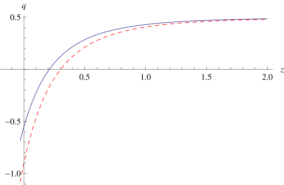
Figure 4: The evolution of deceleration parameter with respect to $z$. For both of the two curves, $\Omega_{m}=0.3$, $\Omega_{k}=0.7$. $Q=0.4$ on the solid curve, and $Q=0.3$ on the dashed curve.

VI conclusion

Our scenario is that the brane is accelerating in the bulk, such that it is bathed in the Unruh radiation in the bulk. The temperature of the Unruh radiation is higher than the brane, which yields energy flux from the Unruh radiation to the brane matter, which accelerates the brane universe.

In this article we study the cosmology case of a DGP braneworld model, that is, an FRW brane imbedded in the bulk spacetime. We first investigate the Unruh temperature that the brane perceives and its “own” temperature. Generally speaking the brane accelerates in the bulk. Hence the particles confined to the brane and inertial on the brane should also perceive Unruh radiation in the bulk. In this paper we show that for a DGP brane in a Minkowski bulk it is just the case. We investigate the case of the brane, as a particle detector, coupled to a massless scalar field in the bulk. As for a point detector, the temperature of the radiation perceived is proportional to the acceleration of the brane.

As for the brane’s own temperature, we should seek a characteristic temperature of the brane. The temperature can reveal the inherent property of gravity. The Friedmann equation can be reproduced by applying the first law of thermal dynamics to the apparent horizon. Thus we take the temperature of the apparent horizon as the characteristic temperature of the brane, which we called geometric temperature.

We find that generally speaking the Unruh temperature the brane perceived and geometric temperature of the brane are not equal. We compare these two temperatures in various cases. We find that for a dust dominated brane, the temperature of the Unruh radiation perceived by a brane is always higher than the geometric temperature of the brane, either in the branch $\epsilon=1$ or $\epsilon=-1$, no matter what the value of the cross radius $r_{c}$ and the spatial curvature of the brane. So, generally speaking the brane and the Unruh radiation it perceived can not reach to thermal equilibrium.

As we pointed out before, the validity of Unruh radiation has been confirmed in detail review ,lin . Therefore if energy exchange is allowed between bulk and matter brane, an energy flux between the bulk radiation and the matter confined to the brane will come forth, which may accelerate our universe. In all cases $\rho>0$, the Unruh temperature of the bulk radiation $T$ is higher than than the geometric temperature $T^{\prime}$ for a dust dominated brane, which means an energy influx to the brane can appear. So we study this possibility in section V.

The DGP braneworld model seems to be a hopeful candidate to explain the cosmological acceleration. But, as we pointed out before, it also suffers from fine-tune problem. To evade this problem, we consider the limiting DGP model, that is, $r_{c}>H_{0}^{-1}$, which means the gravitational effect of the 5th dimension is negligible. Under this condition, the cosmological acceleration does not happen in original DGP model under this situation if there is only dust on the brane. By considering the possible energy influx from the bulk Unruh radiation to the brane induced by the temperature grads, we find the universe can accelerate through interacting the bulk Unruh radiation in a limiting DGP model, even the brane is dust dominated. Differently from previous works on the brane-bulk interaction, we find the interaction form through careful studies on the microscopic mechanism of interaction between brane and bulk. It is shown that the interaction term can be settled up to a constant factor $b$. Based on these constructions we find the acceleration of the brane $A$ is inversely correlated with the energy density of the brane for a dust dominated limiting DGP brane. Finally we derive an exact solution for a spatially flat model. This solution shows clearly that the universe behaves as a dust dominated one at early time and enters a de Sitter phase at late time, which is consistent with observations. We also show the de Sitter phase is stable.

In this paper only massless Unruh mode is considered. Although it is the most important mode in low energy region, the massive mode also deserves to study further for a full Unruh effect in a high energy region. Also, in the enough high energy region, the universe is radiation dominated, and at the same time the scattering cross section between dark matter particles and Unruh photons becomes temperature-dependent, since the internal freedoms can be excited. Under this situation the Unruh effect may be important again, which deserves to investigate further.

At the observation side, we should not only take a special set of parameters to show the property of this model, but constrain the parameters, especially $b$ by various observations in the future.

Acknowledgments. HS Zhang thanks Prof. W. Unruh and Prof. D. Jennings for helpful discussions . H. Noh was supported by grant No. C00022 from the Korea Research Foundation. ZH Zhu was supported by the National Science Foundation of China under the Distinguished Young Scholar Grant 10825313, the Key Project Grant 10533010, and by the Ministry of Science and Technology national basic science Program (Project 973) under grant No. 2007CB815401. HW Yu was supported by the National Natural Science Foundation of China under Grants No. 10575035 and No. 10775050, the SRFDP under Grant No. 20070542002, and the Program for the key discipline in Hunan Province.

References

- (1) A. G. Riess et al., Astron. J. 116, 1009 (1998); S. Perlmutter et al., Astrophys. J. 517, 565 (1999).
- (2) E. J. Copeland, M. Sami and S. Tsujikawa, Int. J. Mod. Phys. D 15, 1753 (2006) [arXiv:hep-th/0603057].
- (3) R. Maartens, Living Rev. Rel. 7, 7 (2004) [arXiv:gr-qc/0312059].
- (4) G. Dvali, G. Gabadadze, M. Porrati, Phys. Lett. B485 (2000) 208 ,hep-th/0005016; G. Dvali and G. Gabadadze, Phys. Rev. D63, 065007 (2001); A. Lue, astro-ph/0510068.
- (5) C. Deffayet, Phys. Lett. B 502, 199 (2001); C. Deffayet, G.Dvali, and G. Gabadadze, Phys. Rev. D 65, 044023 (2002); C.Deffayet, S. J. Landau, J. Raux, M. Zaldarriaga, and P. Astier, Phys. Rev. D 66, 024019 (2002);
- (6) E. Kiritsis, G. Kofinas, N. Tetradis, T.N. Tomaras and V. Zarikas, JHEP 0302 (2003) 035; C. van de Bruck, M. Dorca, 10 C. J. Martins and M. Parry, Phys. Lett. B 495 (2000) 183 ; N. Tetradis, Phys.Lett. B569 (2003) 1; F. K. Diakonos, E. N. Saridakis and N. Tetradis, Phys. Lett. B 605, 1 (2005); E. Kiritsis, JCAP 0510, 014 (2005) ; K. I. Umezu, K. Ichiki, T. Kajino, G. J. Mathews, R. Nakamura and M. Yahiro, Phys. Rev. D73, 063527 (2006); G. Kofinas, G. Panotopoulos and T.N. Tomaras; R. G. Cai, Y. g. Gong and B. Wang, JCAP 0603, 006 (2006).
- (7) D. Jennings, hep-th/0508215.
- (8) J. M. Bardeen, B. Carter and S. W. Hawking, Commun. Math. Phys. 31, 161 (1973).
- (9) S. W. Hawking, Commun. Math. Phys. 43, 199 (1975) [Erratum-ibid. 46, 206 (1976)].
- (10) W.G. Unruh, Phys. Rev. D14, 870 (1976); W.G. Unruh, Phys. Rev. D34, 1222 (1986); W. G. Unruh, Phys. Rev. D 46, 3271 (1992).
- (11) N.D. Birrell, P.C.W. Davies, Quantum fields in curved space (1982), Cambrige university press, Cambrige, UK .
- (12) T. Jacobson, Phys. Rev. Lett. 75, 1260 (1995), gr-qc/9504004.
- (13) R. G. Cai and S. P. Kim, JHEP 0502, 050 (2005) ,hep-th/0501055.
- (14) D. Bak and S. J. Rey, Class. Quant. Grav. 17, L83 (2000) [arXiv:hep-th/9902173]; S. A. Hayward, S. Mukohyama and M. C. Ashworth, Phys. Lett. A 256, 347 (1999) [arXiv:gr-qc/9810006]; S. A. Hayward, Class. Quant. Grav. 15, 3147 (1998) [arXiv:gr-qc/9710089].
- (15) B. S. Kay, Commun. Math. Phys. 100, 57 (1985); R.M. Wald and B. Kay, Phys. Rep. 207, 51 1991; S. De Bievre, M. Merkli, math-ph/0604023.
- (16) P. G. Grove, Classical Quantum Gravity 3, 801 (1986); D. J. Raine, D.W. Sciama, and P. G. Grove, Proc. R. Soc. A 435, 205 (1991).
- (17) W. G. Unruh, Phys. Rev. D 46, 3271 (1992).
- (18) S. Massar, R. Parentani, and R. Brout, Classical Quantum Gravity 10, 385 (1993).
- (19) A. Raval, B. L. Hu, and D. Koks, Phys. Rev. D 55, 4795 (1997).
- (20) S.-Y. Lin, Phys. Rev. D 68, 104019 (2003); S.-Y. Lin and B. L. Hu Phys. Rev. D73, 124018 (2006)
- (21) J. Audretsch and R. Müller, Phys. Rev. A 50, 1755 (1994).
- (22) Z. Zhu, H. Yu and S. Lu, Phys. Rev. D 73, 107501 (2006).
- (23) Z. Zhu and H. Yu, Phys. Lett. B 645, 459 (2007).
- (24) R. Wald, Quantum Field Theory in Curved Space- time and Black Hole Thermodynamics (1994), University of Chicago Press, Chicago, US.
- (25) H. Yu and W. Zhou, Phys. Rev. D 76, 044023 (2007) [arXiv:0707.2613 [gr-qc]]; M. Han, S. J. Olson and J. P. Dowling, arXiv:0705.1350 [quant-ph].
- (26) N. Khosravi, E. Khajeh, R. Rashidi and H. Salehi, Astrophys. Space Sci. 310, 333 (2007) [arXiv:0706.2767 [hep-th]].
- (27) L. C. B. Crispino, A. Higuchi and G. E. A. Matsas, arXiv:0710.5373 [gr-qc].
- (28) Rong-Gen Cai, Hongsheng Zhang, and Anzhong Wang, Commun.Theor.Phys. 44 (2005) 948.
- (29) C. Deffayet, G. Gabadadze and A. Iglesias, JCAP 0608, 012 (2006) [arXiv:hep-th/0607099].
- (30) D. Langlois, Prog.Theor.Phys.Suppl. 148 (2003) 181.
- (31) K. Maeda, S. Mizuno and T. Torii, Phys. Rev. D 68, 024033 (2003).
- (32) S. Alexander, Y. Ling, and L. Smolin Phys. Rev. D 65, 083503 (2002).
- (33) A. Kamenshchik, U. Moschella and V. Pasquier, Phys. Lett. B511 (2001) 265; B. A. Bassett, M. Kunz, D. Parkinson, C. Ungarelli,Phys.Rev. D68 (2003) 043504; S. M. Carroll, V. Duvvuri, M. Trodden and M. S. Turner, Phys. Rev. D 70 (2004) 043528;O. Mena, J. Santiago and J. Weller Phys.Rev.Lett. 96 (2006) 041103; Hongsheng Zhang and Z. H. Zhu, Phys. Rev. D 73, 043518 (2006) [arXiv:astro-ph/0509895].
- (34) K Olive, arXiv:0901.4090.