Quadratic quantum cosmology with Schutz’ perfect fluid

Abstract

We study the classical and quantum models of a Friedmann-Robertson-Walker (FRW) cosmology, coupled to a perfect fluid, in the context of the $f(R)$ gravity. Using the Schutz’ representation for the perfect fluid, we show that, under a particular gauge choice, it may lead to the identification of a time-parameter for the corresponding dynamical system. Moreover, this formalism gives rise to a Schrödinger-Wheeler-DeWitt (SWD) equation for the quantum-mechanical description of the model under consideration, the eigenfunctions of which can be used to construct the wavefunction of the Universe. In the case of $f(R)=R^{2}$ (pure quadratic model), for some particular choices of the perfect fluid source, exact solutions to the SWD equation can be obtained and the corresponding results are compared to the usual $f(R)=R$ model.
PACS numbers: 98.80.Qc, 04.50.+h, 04.60.Ds

1 Introduction

Over the past few years, extended theories of gravity, constructed by adding higher-order curvature terms to the usual Einstein-Hilbert action, have opened a new window to study the accelerated expansion of the universe. It has been shown that such correction terms could give rise to accelerating solutions of the field equations without having to invoke concepts such as dark energy [1]. In a more general setting, one can use a generic function $f(R)$, instead of the usual Ricci scalar $R$, as the action of gravitational field. In more recent times, such $f(R)$ gravity theories have been extensively studied in the literature, see [2] for a review.

In fact, quadratic and higher-order gravity theories have been used long before the accelerated expansion of the Universe is observed, immediately after Lovelock’s natural generalization of the Einstein-Hilbert action for the gravitational field [3]. Quadratic Lagrangians, in particular, have been used to yield renormalizable theories of gravity coupled to matter [4]. They can also help us to improve the semiclassical approximation, where quantized matter fields interact with the classical gravitational field [5]. In this context, renormalization of the energy-momentum tensor for a quantum field in a four-dimensional, curved space-time indicates that the presence of quadratic terms in the gravitational action is a priori expected [6]. On the other hand, Kleidis et al [7], demonstrated that, in quadratic gravity theories, an additional coupling arises between $R^{2}$ and any massive quantum scalar field, introducing a geometric source term in the wave equation for the quantum field.

In order to find the dynamical equations of motion one can vary the action with respect to the metric (metric formalism), or view the metric and connections as independent dynamical variables and vary the action with respect to both independently (Palatini formalism) [8]. One should note that, although in the usual Einstein-Hilbert action these two approaches give the same field equations, in $f(R)$ gravity the Palatini formalism leads to different dynamical equations due to nonlinear terms in the action. However, the $f(R)$ form of the action is shown to be equivalent to a scalar-tensor type theory and there is an equivalence between the metric and the Palatini $f(R)$ gravity with Brans-Dicke theories. Indeed, one can show that these versions of $f(R)$ gravity are dynamically equivalent to the Brans-Dicke theory of gravity with values of the Brans-Dicke parameter $\omega=0$ and $\omega=-3/2$, respectively [2], [9]. There is also a third version of $f(R)$ gravity in which the Lagrangian of the matter depends on the connections of the metric (metric-affine formalism) [10].

It becomes evident that, the corrections of the $f(R)$-gravity to the results of the standard general relativity have been widely investigated, but, most of these works are restricted in the classical regime [11]. The cases dealing with quantum $f(R)$ models have seldom been studied in the literature [12], and it would be of interest to employ such models in this study.

In this paper we shall investigate the problem of quantization of a FRW cosmological model in the context of $f(R)$ cosmology. For the matter field coupled to gravity we consider a perfect fluid in Schutz’ formalism [13]. The advantage of using this formalism in our quantum cosmological model is that, in a natural way, it can offer a time parameter in terms of dynamical variables of the perfect fluid [14]. Indeed, as we shall show, after a canonical transformation the conjugate momentum associated to one of the variables of the fluid appears linearly in the Hamiltonian of the model. Therefore, canonical quantization results in a Schrödinger-Wheeler-DeWitt (SWD) equation, in which this matter variable plays the role of time. However, it should be emphasized that we do not deal with the problem of time in the quantum cosmology of the model at hand in a fundamental way. As are well known, quantum cosmology suffers from a number of problems which one of the most important of them is the problem of time, i.e., the wave function in the Wheeler-DeWitt equation is independent of time and thus the Universe has a static picture in this scenario. This problem was first addressed in [15] by DeWitt himself. He argued that the problem of time should not be considered as a hindrance in the sense that the theory itself must include a suitable well-defined time in terms of its geometry or matter fields. Therefore, since by the Wheeler-DeWitt approach one can find different time parameters directly from the the super-metric, the sole purpose of the use of a perfect fluid instead of a field with its own degrees of freedom seems to be the emergence of a Schrödinger-type equation with a time parameter $t$, which is not the case for the general Wheeler-DeWitt equation. The Schutz model is thus of limited value in view of the problem of time in quantum cosmology.

Here, we first consider a generic form of $f(R)$ function in the FRW background with a generic equation of state for the perfect fluid to construct the phase space of the model. As we find out, even for the simplest forms of the $f(R)$-function, the corresponding SWD equation is too complicated to be solved in terms of analytic functions. Therefore, we restrict ourselves to a pure fourth order model, in which $f(R)=R^{2}$. Accordingly, we show that, for some special forms of the equation of state of the perfect fluid, the SWD equation can be solved exactly in terms of known special functions. We then construct the resulting wavefunction of the universe in this quadratic framework and compare its similarities and differences with usual $f(R)=R$ model. It is to be noted that our presentation does not claim to deal with $f(R)$ quantum cosmology in a fundamental way since we study the problem in a simple toy model. However, this study may reflect realistic scenarios in other similar investigations, dealing with such problems in a more fundamental way.

2 The phase space of the model

In this section we consider a FRW cosmology within the framework of $f(R)$ gravity. In the context of the ADM formalism, the action for gravity coupled to a perfect fluid in Schutz’ representation is written as (in what follows we work in units where $c=\hbar=16\pi G=1$)

$${\cal S}=\int_{M}d^{4}x\sqrt{-g}f(R)+2\int_{\partial M}d^{3}x\sqrt{h}h_{ab}K^{ab}+\int_{M}d^{4}x\sqrt{-g}p,$$ (1)

where $R$ is the scalar curvature and $f(R)$ is an arbitrary function of $R$. Also, $K^{ab}$ is the extrinsic curvature and $h_{ab}$ is the induced metric over the three dimensional spatial hypersurface, which is the boundary $\partial M$ of the four dimensional manifold $M$. The last term of (1) denotes the matter contribution to the total action where $p$ is the pressure of perfect fluid which is linked to its energy density by the equation of state

$$p=\alpha\rho.$$ (2)

In Schutz’ formalism [13], the fluid’s four-velocity is expressed in terms of five potentials $\epsilon$, $\zeta$, $\beta$, $\theta$ and $S$ as

$$U_{\nu}=\frac{1}{\mu}(\epsilon_{,\nu}+\zeta\beta_{,\nu}+\theta S_{,\nu}),$$ (3)

where $\mu$ is the specific enthalpy, the variable $S$ is the specific entropy while the potentials $\zeta$ and $\beta$ are related to torsion and are absent in the FRW models. The variables $\epsilon$ and $\theta$ have no clear physical interpretation in this formalism. The four-velocity satisfies the condition

$$U^{\nu}U_{\nu}=-1.$$ (4)

We assume that the geometry of space time is described by the FRW metric

$$ds^{2}=-N^{2}(t)dt^{2}+a^{2}(t)\left[\frac{dr^{2}}{1-kr^{2}}+r^{2}(d\vartheta^{2}+\sin^{2}\vartheta d\varphi^{2})\right],$$ (5)

where $N(t)$ is the lapse function, $a(t)$ the scale factor and $k$=$1$, $0$ and $-1$ correspond to the closed, flat and open universe respectively. To proceed further, we need an effective Lagrangian for the model whose variation with respect to its dynamical variables yields the appropriate equations of motion. Therefore, by considering the above action as representing a dynamical system in which the scale factor $a$, scalar curvature $R$ and fluid’s potentials play the role of independent dynamical variables, we can rewrite the gravitational part of action (1) as

$${\cal S}_{grav}=\int dt{\cal L}_{grav}(a,\dot{a},R,\dot{R})=\int dt\left\{Na^{3}f(R)-\lambda\left[R-\frac{6}{N^{2}}\left(\frac{\ddot{a}}{a}+\frac{\dot{a}^{2}}{a^{2}}+\frac{k}{a^{2}}-\frac{\dot{N}\dot{a}}{Na}\right)\right]\right\},$$ (6)

where we have introduced the definition of $R$ in terms of $a$ and its derivatives as a constraint. This procedure allows us to remove the second order derivatives from action (6). The Lagrange multiplier $\lambda$ can be obtained by variation with respect to $R$, that is, $\lambda=Na^{3}f^{\prime}(R)$, in which a prime denotes the derivative with respect to $R$ . Thus, we obtain the following point-like Lagrangian for the gravitational part of the model

$${\cal L}_{grav}=-\frac{6}{N}a\dot{a}^{2}f^{\prime}-\frac{6}{N}a^{2}\dot{a}\dot{R}f^{\prime\prime}+6kNaf^{\prime}+Na^{3}(f-Rf^{\prime}).$$ (7)

To simplify this Lagrangian, we define the variable $\phi$ as $f^{\prime}(R)=\phi$, in terms of which the Lagrangian (7) reads

$${\cal L}_{grav}=-\frac{6}{N}a\dot{a}^{2}\phi-\frac{6}{N}a^{2}\dot{a}\dot{\phi}+6kNa\phi-Na^{3}V(\phi),$$ (8)

where $V(\phi)=Rf^{\prime}-f=R\phi-f$.

Also, the matter part of the action (1) becomes ${\cal S}_{matt}=\int d^{3}xdtNa^{3}p$, so the Lagrangian density of the fluid is ${\cal L}_{matt}=Na^{3}p$. Following the thermodynamic description of [13], the basic thermodynamic relations take the form

$$\rho=\rho_{0}(1+\Pi),\hskip 14.22636pt\mu=1+\Pi+\frac{p}{\rho_{0}},$$ (9)

where $\rho_{0}$ and $\Pi$ are the rest-mass density and the specific internal energy of the fluid respectively. These quantities together with the temperature of the system $\tau$, obey the first law of the thermodynamics $\tau dS=d\Pi+pd(1/\rho_{0})$, where can be rewritten as

$$\tau dS=d\Pi+pd\left(\frac{1}{\rho_{0}}\right)=(1+\Pi)d\left[\ln\rho_{0}^{-\alpha}(1+\Pi)\right],$$ (10)

in which we have used the equation of state (2). Therefore, we obtain the following expressions for the temperature and the entropy of the fluid

$$\tau=1+\Pi,\hskip 14.22636ptS=\ln\rho_{0}^{-\alpha}(1+\Pi)=\ln\frac{\mu}{\alpha+1}\rho_{0}^{-\alpha}.$$ (11)

Now, we can express $\rho_{0}$ and $\Pi$ as functions of $\mu$ and $S$ as

$$1+\Pi=\frac{\mu}{\alpha+1},\hskip 14.22636pt\rho_{0}=\left(\frac{\mu}{\alpha+1}\right)^{1/\alpha}e^{-S/\alpha},$$ (12)

so that with the help of (9), one can put the equation of state in the form

$$p=\frac{\alpha}{(\alpha+1)^{1+1/\alpha}}\mu^{1+1/\alpha}e^{-S/\alpha}.$$ (13)

On the other hand, normalization of the fluid’s four-velocity (3), according to the relation (4) implies $\mu=(\dot{\epsilon}+\theta\dot{S})/N$. Therefore, using the above constraints and thermodynamical considerations for the fluid we find

$${\cal L}_{matt}=N^{-1/\alpha}a^{3}\frac{\alpha}{(\alpha+1)^{1+1/\alpha}}\left(\dot{\epsilon}+\theta\dot{S}\right)^{1+1/\alpha}e^{-S/\alpha}.$$ (14)

Let us now construct the Hamiltonian for our model. The momenta conjugate to each of the above variables can be obtained from the definition $P_{q}=\frac{\partial{\cal L}}{\partial\dot{q}}$. In terms of the conjugate momenta the Hamiltonian is given by

$$H=H_{grav}+H_{matt}=\dot{a}P_{a}+\dot{\phi}P_{\phi}+\dot{\epsilon}P_{\epsilon}+\dot{S}P_{S}-{\cal L},$$ (15)

where ${\cal L}={\cal L}_{grav}+{\cal L}_{matt}$. Noting that

$$P_{\epsilon}=\frac{\partial{\cal L}}{\partial\dot{\epsilon}}=N^{-1/\alpha}a^{3}\frac{(\dot{\epsilon}+\theta\dot{S})^{1/\alpha}}{(\alpha+1)^{1/\alpha}}e^{-S/\alpha},$$

and

$$P_{S}=\frac{\partial{\cal L}}{\partial\dot{S}}=N^{-1/\alpha}a^{3}\frac{(\dot{\epsilon}+\theta\dot{S})^{1/\alpha}}{(\alpha+1)^{1/\alpha}}\theta e^{-S/\alpha},$$

expression (15) leads

$$H=N{\cal H}=N\left[-\frac{P_{a}P_{\phi}}{6a^{2}}+\frac{\phi}{6a^{3}}P_{\phi}^{2}-6ka\phi+a^{3}V(\phi)+a^{-3\alpha}e^{S}P_{\epsilon}^{\alpha+1}\right].$$ (16)

Now, consider the following canonical transformation which is a generalization of the ones used in [16]

$$\begin{array}[]{cc}T=-P_{S}e^{-S}P_{\epsilon}^{-(\alpha+1)},&P_{T}=P_{\epsilon}^{\alpha+1}e^{S},\\ \\ \bar{\epsilon}=\epsilon-(\alpha+1)\frac{P_{S}}{P_{\epsilon}},&\bar{P_{\epsilon}}=P_{\epsilon}.\end{array}$$ (17)

Under this transformation Hamiltonian (16) takes the form

$$H=N{\cal H}=N\left[-\frac{P_{a}P_{\phi}}{6a^{2}}+\frac{\phi}{6a^{3}}P_{\phi}^{2}-6ka\phi+a^{3}V(\phi)+\frac{P_{T}}{a^{3\alpha}}\right].$$ (18)

We see that the momentum $P_{T}$ is the only remaining canonical variable associated with matter and appears linearly in the Hamiltonian. The setup for constructing the phase space and writing the Lagrangian and Hamiltonian of the model is now complete.

The classical dynamics is governed by the Hamiltonian equations, that is

$$\left\{\begin{array}[]{ll}\dot{a}=\{a,H\}=-\frac{N}{6}\frac{P_{\phi}}{a^{2}},\\ \\ \dot{P_{a}}=\{P_{a},H\}=N\left[-\frac{1}{3}a^{-3}P_{a}P_{\phi}+\frac{1}{2}\phi a^{-4}P_{\phi}^{2}+6k\phi-3a^{2}V(\phi)+3\alpha a^{-3\alpha-1}P_{T}\right],\\ \\ \dot{\phi}=\{\phi,H\}=N\left[-\frac{1}{6}\frac{P_{a}}{a^{2}}+\frac{1}{3}\frac{\phi}{a^{3}}P_{\phi}\right],\\ \\ \dot{P_{\phi}}=\{P_{\phi},H\}=N\left[-\frac{1}{6}\frac{P_{\phi}^{2}}{a^{3}}+6ka-a^{3}V^{\prime}(\phi)\right],\\ \\ \dot{T}=\{T,H\}=\frac{N}{a^{3\alpha}},\\ \\ \dot{P_{T}}=\{P_{T},H\}=0.\end{array}\right.$$ (30)

We also have the constraint equation ${\cal H}=0$. Up to this point the cosmological model, in view of the concerning issue of time, has been of course under-determined. Before trying to solve these equations we must decide on a choice of time in the theory. The under-determinacy problem at the classical level may be removed by using the gauge freedom via fixing the gauge. A glance at the above equations shows that choosing the gauge $N=a^{3\alpha}$, we have

$$N=a^{3\alpha}\Rightarrow T=t,$$ (31)

which means that variable $T$ may play the role of time in the model. Therefore, the classical equations of motion can be rewritten in the gauge $N=a^{3\alpha}$ as follows

$$\left\{\begin{array}[]{ll}\dot{a}=-\frac{1}{6}a^{3\alpha-2}P_{\phi},\\ \\ \dot{P_{a}}=-\frac{1}{3}a^{3\alpha-3}P_{a}P_{\phi}+\frac{1}{2}\phi a^{3\alpha-4}P_{\phi}^{2}+6ka^{3\alpha}\phi-3a^{3\alpha+2}V(\phi)+3\alpha a^{-1}P_{0},\\ \\ \dot{\phi}=-\frac{1}{6}a^{3\alpha-2}P_{a}+\frac{1}{3}a^{3\alpha-3}\phi P_{\phi},\\ \\ \dot{P_{\phi}}=-\frac{1}{6}a^{3\alpha-3}P_{\phi}^{2}+6ka^{3\alpha+1}-a^{3\alpha+3}V^{\prime}(\phi),\end{array}\right.$$ (39)

where we take $P_{T}=P_{0}=\mbox{const.}$ from the last equation of (30). Since integrability of this system directly depends on the choice of a form for $f(R)$ (which determines potential $V(\phi)$), it is appropriate to concentrate on this point first. However, before choosing such a function, let us deal with the quantum cosmology of the model described above.

3 Quantization of the model

We now focus attention on the study of the quantum cosmology of the model described above. We start by writing the Wheeler-DeWitt equation from Hamiltonian (18). Since the lapse function $N$ appears as a Lagrange multiplier in this Hamiltonian, we have the Hamiltonian constraint ${\cal H}=0$. Thus, application of the Dirac quantization procedure demands that the quantum states of the Universe should be annihilated by the operator version of ${\cal H}$, that is

$${\cal H}\Psi(a,\phi,T)=\left[-\frac{P_{a}P_{\phi}}{6a^{2}}+\frac{\phi}{6a^{3}}P_{\phi}^{2}-6ka\phi+a^{3}V(\phi)+\frac{P_{T}}{a^{3\alpha}}\right]\Psi(a,\phi,T)=0,$$ (40)

where $\Psi(a,\phi,T)$ is the wavefunction of the universe. A remark about the reduced Hamiltonian in the above procedure is the factor-ordering problem when one embarks on constructing a quantum mechanical operator equation. In dealing with such Hamiltonians at the quantum level extra care should be taken when one tries to replace the dynamical variables with their quantum operator counterparts, that is , in replacing a variable $q$ and its momentum $p_{q}$ with their corresponding operators, the ordering considerations should be taken into account. Therefore, to guarantee Hermiticity, the operator form corresponding to equation (40) may be written as

$$\left[-\frac{1}{12}\left(a^{r}P_{a}a^{s}+a^{s}P_{a}a^{r}\right)P_{\phi}+\frac{1}{12a^{3}}\left(\phi^{u}P_{\phi}\phi^{v}P_{\phi}\phi^{w}+\phi^{w}P_{\phi}\phi^{v}P_{\phi}\phi^{u}\right)\right.$$

$$\left.-6ka\phi+a^{3}V(\phi)+\frac{P_{T}}{a^{3\alpha}}\right]\Psi(a,\phi,T)=0,$$ (41)

where the parameters $r$, $s$, $u$, $v$ and $w$ satisfy $r+s=-2$, $u+v+w=1$ and denote the ambiguity in the ordering of factors $a$ and $P_{a}$ in the first and $\phi$ and $P_{\phi}$ in the second term of (40). With the replacement $P_{a}\rightarrow-i\frac{\partial}{\partial a}$ and similarly for $P_{\phi}$ and $P_{T}$ the above equation reads

$$\left[\frac{1}{6}a^{-2}\frac{\partial^{2}}{\partial a\partial\phi}-\frac{1}{3}a^{-3}\frac{\partial}{\partial\phi}-\frac{1}{6}a^{-3}\phi\frac{\partial^{2}}{\partial\phi^{2}}+\frac{1}{6}A\phi^{-1}a^{-3}-6ka\phi\right.$$

$$\left.+a^{3}V(\phi)-a^{-3\alpha}i\frac{\partial}{\partial T}\right]\Psi(a,\phi,T)=0,$$ (42)

where $A=uw$. This equation takes the form of a Schrödinger equation $i\partial\Psi/\partial T=H\Psi$, in which the new Hamiltonian operator is Hermitian for any choice of the ordering parameters with the standard inner product

$$<\Phi\mid\Psi>=\int_{(a,\phi)}a^{-3\alpha}\Phi^{\ast}\Psi dad\phi.$$ (43)

We separate the variables in the SWD equation (3) as

$$\Psi(a,\phi,T)=e^{-iET}\psi(a,\phi),$$ (44)

leading to

$$\left\{a\phi\frac{\partial^{2}}{\partial a\partial\phi}-\phi^{2}\frac{\partial^{2}}{\partial\phi^{2}}-2\phi\frac{\partial}{\partial\phi}+\left[A-36ka^{4}\phi^{2}+6a^{6}\phi V(\phi)-6Ea^{3-3\alpha}\phi\right]\right\}\psi(a,\phi)=0,$$ (45)

where $E$ is a separation constant. It is seen that this equation has a mixed derivative with respect to the variables $a$ and $\phi$ and also, these variables appear in a mixed form in the last term of the equation. Under these conditions equation (45) cannot be solved by the method of separation of variables. Therefore, it is useful to introduce the following change of variables

$$x=a\phi^{1/2},\hskip 14.22636pty=\phi.$$ (46)

In terms of these variables equation (45) takes the form

$$\left\{\frac{1}{4}x^{2}\frac{\partial^{2}}{\partial x^{2}}-\frac{1}{4}x\frac{\partial}{\partial x}-y^{2}\frac{\partial^{2}}{\partial y^{2}}-2y\frac{\partial}{\partial y}+\left[A-36kx^{4}+6x^{6}y^{-2}V(y)-6Ex^{3-3\alpha}y^{\frac{1}{2}(3\alpha-1)}\right]\right\}\psi(x,y)=0.$$ (47)

Unfortunately, this equation cannot be solved analytically for an arbitrary potential function $V(y)$ and parameter $\alpha$, which represent the form of $f(R)$ and the nature of the perfect fluid respectively. In the next section we shall present a class of exact solutions for this equation in pure $R^{2}$ cosmology for two special cases of perfect fluid.

4 Quantum solutions for $f(R)=R^{2}$ cosmology

For the pure fourth order ($f(R)=R^{2}$), model we have $\phi=f^{\prime}(R)=2R$ and $V(\phi)=Rf^{\prime}-f=R^{2}$. Hence, from (46) we obtain $V(\phi)=\frac{1}{4}\phi^{2}=\frac{1}{4}y^{2}$. Therefore, equation (47) reduces to

$$\left\{\frac{1}{4}x^{2}\frac{\partial^{2}}{\partial x^{2}}-\frac{1}{4}x\frac{\partial}{\partial x}-y^{2}\frac{\partial^{2}}{\partial y^{2}}-2y\frac{\partial}{\partial y}+\left[A-36kx^{4}+\frac{3}{2}x^{6}-6Ex^{3-3\alpha}y^{\frac{1}{2}(3\alpha-1)}\right]\right\}\psi(x,y)=0.$$ (48)

It is seen that in the cases of $\alpha=1,1/3$, the variables $x$ and $y$ can be separated from each other and equation (48) may be solved analytically for these two cases. Thus, in what follows we restrict ourselves to these two special cases.

4.1 Stiff matter: $\alpha=1$

Stiff matter is a fluid with pressure equal to energy density and speed of sound equal to speed of light. In this case we separate the solutions of equation (48) into the form $\psi(x,y)=X(x)Y(y)$ leading to

$$\left\{\begin{array}[]{ll}\left[x^{2}\frac{d^{2}}{dx^{2}}-x\frac{d}{dx}+\left(1-\nu^{2}-144kx^{4}+6x^{6}\right)\right]X(x)=0,\\ \\ \left[y^{2}\frac{d^{2}}{dy^{2}}+2y\frac{d}{dy}+\left(6Ey-\frac{\nu^{2}-1}{4}\right)\right]Y(y)=0,\end{array}\right.$$ (52)

where we take $\frac{\nu^{2}-1}{4}$ as a separation constant and also $A=0$ without losing general character of the wavefunction. One should note that there exists an infinite number of possibilities of ordering. As Hawking and Page have shown [18], the factor ordering parameter will not affect semiclassical calculations in quantum cosmology and so for convenience one usually choose a special value for it in the special models. On the other hand, in general, the behavior of the wavefunction depends on the chosen factor ordering [19]. But in the model at hand, as is clear from equation (48), the factor $A$ will appear in the solutions of (52) only together with the separation constant $\nu$ (for example $\nu\rightarrow\sqrt{\nu^{2}-4A}$ in the first equation of (52)). Therefore, since we finally take a superposition over all values of this separation constant, we expect that the essential features of the wavefunction will remain the same for different choices of the factor ordering parameter $A$. Also, with an eye to equation (3), it is to be noted that the choice $A=0$ yields a zero value for $u$ or $w$ or both of them. In all of these cases the Hermiticity of the second term in equation (3) will remain unchanged. From this point of view the particular choice $A=0$ does not reflect major effects to equation (3).

For the flat FRW metric ($k=0$), the above equations have the following solutions in terms of Bessel functions

$$\left\{\begin{array}[]{ll}X(x)=x\left[c_{1}J_{\frac{\nu}{3}}\left(\sqrt{\frac{2}{3}}x^{3}\right)+c_{2}Y_{\frac{\nu}{3}}\left(\sqrt{\frac{2}{3}}x^{3}\right)\right],\\ \\ Y(y)=\frac{1}{\sqrt{y}}\left[d_{1}J_{\nu}\left(\sqrt{24Ey}\right)+d_{2}Y_{\nu}\left(\sqrt{24Ey}\right)\right],\end{array}\right.$$ (56)

where $c_{i}$ and $d_{i}$ ($i=1,2$) are integration constants. Thus, the eigenfunctions of the SWD equation for stiff matter, can be written as

$$\Psi_{\nu E}(x,y,T)=e^{-iET}\frac{x}{\sqrt{y}}J_{\frac{\nu}{3}}\left(\sqrt{\frac{2}{3}}x^{3}\right)J_{\nu}\left(\sqrt{24Ey}\right),$$ (57)

where we choose $c_{2}=d_{2}=0$ for having well-defined functions in all ranges of variables $x$ and $y$. We may now write the general solutions to the SWD equations as a superposition of the eigenfunctions, that is

$$\Psi(x,y,T)=\int_{E=0}^{\infty}\int_{\nu=0}^{\infty}A(E)C(\nu)\Psi_{\nu E}(x,y,T)dEd\nu,$$ (58)

in which $A(E)$ and $C(\nu)$ are suitable weight functions to construct the wave packets. By using the equality [20]

$$\int_{0}^{\infty}e^{-ar^{2}}r^{\nu+1}J_{\nu}(br)dr=\frac{b^{\nu}}{(2a)^{\nu+1}}e^{-\frac{b^{2}}{4a}},$$ (59)

we can evaluate the integral over $E$ in (58) and simple analytical expression for this integral is found if we choose the function $A(E)$ to be a quasi-Gaussian weight factor $A(E)=12(24E)^{\nu/2}e^{-24\gamma E}$, which results in

$$\int_{0}^{\infty}A(E)e^{-iET}J_{\nu}\left(\sqrt{24Ey}\right)dE=\frac{y^{\nu/2}}{\left(2\gamma+\frac{iT}{12}\right)^{\nu+1}}\mbox{exp}\left(-\frac{y}{4\gamma+\frac{iT}{6}}\right),$$ (60)

where $\gamma$ is an arbitrary positive constant. Substitution of the above relation into equation (58) leads to the following expression for the wavefunction

$$\Psi(x,y,T)=\frac{x}{\sqrt{y}}\mbox{exp}\left(-\frac{y}{4\gamma+\frac{iT}{6}}\right)\int_{0}^{\infty}C(\nu)\frac{y^{\nu/2}}{\left(2\gamma+\frac{iT}{12}\right)^{\nu+1}}J_{\frac{\nu}{3}}\left(\sqrt{\frac{2}{3}}x^{3}\right)d\nu,$$ (61)

where $C(\nu)$ can now be chosen as a shifted Gaussian weight function $e^{-a(\nu-b)^{2}}$. It is seen that this expression is too complicated for extracting an analytical closed form for the wavefunction and the choice of a function $C(\nu)$ that leads to an analytical solution for the wavefunction is not an easy task. In this respect, our choices for $A(E)$ and $C(\nu)$ as quasi-Gaussian and shifted Gaussian weight functions respectively, appear to have physical grounds. Such Gaussian weight functions are widely used in quantum mechanics as a way to think about the localized states. This is because that these types of weight factors are centered about a special value of their argument and they fall off rapidly away from that center. Due to this behavior the corresponding wave packet resulting from (61) after integration, has also a Gaussian-like behavior, i.e., is localized about some special values of its arguments. Therefore, it is seen that there is a reciprocal relation between the width of the Gaussian weight function that determines the shape of the wave packet, and the width of the wave packet. In this sense the motion of the peaks of the wave packets with a group velocity and also its spreading behavior (see below), can be best seen in terms of the Gaussian packets.

In figure 1 we have plotted the square of the wavefunction for typical numerical values of the parameters.

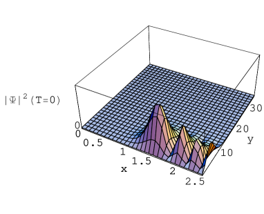
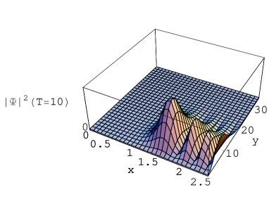
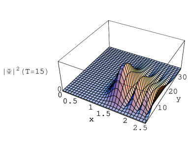
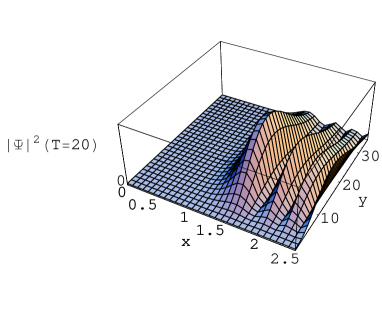
Figure 1: The figures show $|\Psi(x,y,T)|^{2}$, the square of the wavefunction in four different time parameter $T=0,10,15,20$. The figures are plotted for the numerical values $a=2$, $b=5$ and $\gamma=0.5$, and we have taken the integral in (61) from $0$ to $10$.

As this figure shows, at $T=0$, the wavefunction has a dominant peak in the vicinity of some nonzero values of $x$ and $y$ followed by smaller peaks, which as $x$ grows, their amplitudes are suppressed. This means that the wavefunction predicts the emergence of the universe from a state corresponding to its dominant peak. However, the emergence of several peaks in the wave packet may be interpreted as a representation of different quantum states that may communicate with each other through tunneling. This means that there are different possible universes (states) from which our present universe could have evolved and tunneled in the past, from one universe (state) to another. As time progresses, the wave packet begins to propagate in the $y$-direction, its width becoming wider and its peaks moving with a group velocity towards the greater values of $y$. Bearing in mind that $y=\phi=f^{\prime}(R)$, this wavefunction predicts that the universe will assume states with larger $R$ in its late time evolution.

Before going any further, let us take a look at the classical cosmology corresponding to the above quantum solutions. For the quadratic model, we insert $V(\phi)=\frac{1}{4}\phi^{2}$ in the system (39), take $\alpha=1$ for the matter character and also $k=0$ representing the flat FRW space time. We see that the classical cosmology forms a system of nonlinear coupled differential equations which unfortunately cannot be solved analytically. In figure 2, employing numerical methods, we have shown the approximate behavior of $a(t)$, $x(t)$ and $\phi(t)\sim R(t)$ for typical values of the parameters and initial conditions respectively.

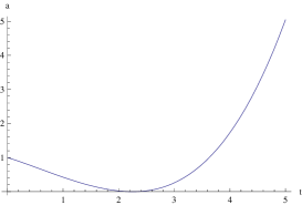
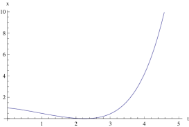
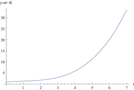
Figure 2: Approximate behavior of $a(t)$, the scale factor, $x(t)=a\phi^{1/2}$ and $R(t)$, the Ricci scalar, in the classical cosmology framework. The figures are plotted for numerical values $\alpha=1$, $k=0$ and $P_{0}=1$. We take the initial conditions $a(t=0)=\phi(t=0)=1$ and $P_{a}(t=0)=P_{\phi}(t=0)=3$. After examining other sets of initial conditions, we verify that this behavior repeats itself.

As is clear from the figures, while the Ricci scalar has a monotonically growing behavior with time, the scale factor first decreases and then increases forever. On the other hand, take a look at the figure 1 shows that the quantum states with larger (smaller) peaks, i.e., the states of high (low) probability, are located at the smaller (larger) values for the scale factor. Therefore, when the scale factor decreases (increases) with time in the classical point of view, in the quantum domain tunneling occurs from a state with a smaller (larger) peak to another with a larger (smaller) one. Also, in view of the behavior of the Ricci scalar, the classical and quantum solutions are in complete agreement with each other and both predict a monotonically increasing evolution for this variable. Therefore, it is seen that there is an almost good correlation between the quantum patterns shown in figure 1 and classical trajectories. However, in order to show this correlation in a more clear sense, one may calculate the time dependence of the expectation values. As we have seen in the second section, the variable $T$ can be regarded as an internal clock for the dynamics. The effective (reduced) Hamiltonian for this system can be found by solving the constraint ${\cal H}=0$ for $\pm P_{T}$ [21]. Hence

$$H_{eff}=-\frac{1}{6}a^{3\alpha-2}P_{a}P_{\phi}+\frac{1}{6}a^{3\alpha-3}\phi P_{\phi}^{2}-6ka^{3\alpha+1}\phi+a^{3\alpha+3}V(\phi).$$ (62)

With respect to this Hamiltonian the time evolution of the expectation value of an observable ${\cal O}$ reads as $\frac{d<{\cal O}>}{dT}=-i<\left[{\cal O},H_{eff}\right]>$. Therefore, we get

$$\left\{\begin{array}[]{ll}\frac{d<a>}{dT}=-\frac{1}{6}<a^{3\alpha-2}P_{\phi}>,\\ \\ \frac{d<P_{a}>}{dT}=-\frac{1}{3}<a^{3\alpha-3}P_{a}P_{\phi}>+\frac{1}{2}<\phi a^{3\alpha-4}P_{\phi}^{2}>+6k<a^{3\alpha}\phi>\\ -3<a^{3\alpha+2}V(\phi)>+3\alpha P_{0}<a^{-1}>,\\ \\ \frac{d<\phi>}{dT}=-\frac{1}{6}<a^{3\alpha-2}P_{a}>+\frac{1}{3}<a^{3\alpha-3}\phi P_{\phi}>,\\ \\ \frac{d<P_{\phi}>}{dT}=-\frac{1}{6}<a^{3\alpha-3}P_{\phi}^{2}>+6k<a^{3\alpha+1}>-<a^{3\alpha+3}V^{\prime}(\phi)>.\end{array}\right.$$ (71)

In the case of a very localized wave packet as we have constructed in figure 1 (see also figure 3 in the next subsection) a function $\Omega({\cal O},P)$ varies very little over the size of the wave packet and thus the approximation $<\Omega({\cal O},P)>\sim\Omega(<{\cal O}>,<P>)$ holds. Under this condition the trajectories for the expectation values obtained from the system (71) are in agreement with the classical ones obtained from the system (39) and shown in figures 2, 4. To summarize, in the present case where we have localized wave packets the expectation value of the scale factor is very close to the classical one and thus $<a>$ follows the pattern of $a(t)$ shown in figure 2 with a good approximation.

4.2 Radiation: $\alpha=1/3$

In the standard Big-Bang model, it is believed that the early universe is dominated either by radiation or radiation and high energy particles. Since in this era the temperature is above electron-positron pair threshold, these particles are relativistic and the whole mixture behaves more like radiation rather than matter. When the cosmological fluid is dominated by radiation, as it was presumably the case in the early universe, the equation of state can be taken as $p=\rho/3$. In this case, the solutions of equation (48) may be again separated into the form $\psi(x,y)=X(x)Y(y)$ leading to

$$\left\{\begin{array}[]{ll}\left[x^{2}\frac{d^{2}}{dx^{2}}-x\frac{d}{dx}+\left(1-4\nu^{2}-144kx^{4}+6x^{6}-24Ex^{2}\right)\right]X(x)=0,\\ \\ \left[y^{2}\frac{d^{2}}{dy^{2}}+2y\frac{d}{dy}+\nu^{2}-\frac{1}{4}\right]Y(y)=0,\end{array}\right.$$ (75)

where we take $1-4\nu^{2}$ as a separation constant. Similar to the previous subsection, we deal again with the solutions of the above system in the case when $k=0$. In general, although the second equation of the system (75) has exact solutions, its first equation cannot be solved analytically. However, as we mentioned above, the radiation is not the dominant fluid at the present epoch but was dominant in early universe, i.e., in the regime where the scale factor is expected to have a small value. On the other hand, our classical analysis in this case (see below and figure 4) will show that the Ricci scalar follows a vanishing value. Therefore, we may write $x^{2}=a^{2}(2R)\sim\xi\ll 1$ and hence $x^{6}=a^{6}(2R)^{3}\sim\xi a^{4}(2R)^{2}=\xi x^{4}$. Thus, we use the approximation $x^{6}\sim\xi x^{4}$ in this era and rewrite the SWD equation as

$$\left\{\begin{array}[]{ll}\left[x^{2}\frac{d^{2}}{dx^{2}}-x\frac{d}{dx}+\left(1-4\nu^{2}+6\xi x^{4}-24Ex^{2}\right)\right]X(x)=0,\\ \\ \left[y^{2}\frac{d^{2}}{dy^{2}}+2y\frac{d}{dy}+\frac{1}{4}-\nu^{2}\right]Y(y)=0.\end{array}\right.$$ (79)

Now, the first equation of the system has well known solutions in terms of confluent hypergeometric functions $M(a,b;x)$ and $U(a,b;x)$. Therefore, we get

$$X(x) = (i\sqrt{6\xi}x^{2})^{\nu+1/2}e^{-i\frac{\sqrt{6\xi}}{2}x^{2}}$$ (80)

$$\times\left[C_{1}U\left(\nu+\frac{1}{2}-i\sqrt{6}E,2\nu+1;i\sqrt{6\xi}x^{2}\right)+C_{2}M\left(\nu+\frac{1}{2}-i\sqrt{6}E,2\nu+1;i\sqrt{6\xi}x^{2}\right)\right],$$

$$Y(y)=D_{1}y^{\nu-1/2}+D_{2}y^{-\nu-1/2},$$ (81)

where $C_{i}$ and $D_{i}$ ($i=1,2$) are integration constants. Thus, the SWD equation for radiation fluid has the following eigenfunctions

$$\Psi_{\nu E}(x,y,T)=e^{-iET}x^{2\nu+1}e^{-i\frac{\sqrt{6\xi}}{2}x^{2}}M\left(\nu+\frac{1}{2}-i\sqrt{6}E,2\nu+1;i\sqrt{6\xi}x^{2}\right)y^{-\nu-1/2},$$ (82)

where we take $C_{1}=D_{1}=0$ to have well-defined eigenfunctions for constructing the wave packets. To construct such wave packets since the weight functions can be chosen as a shifted Gaussian function, the general solutions to the SWD equation read as

$$\Psi(x,y,T)=\int_{\nu=0}^{\infty}\int_{E=0}^{\infty}e^{-\sigma(\nu-\nu_{0})^{2}}e^{-\varsigma(E-E_{0})^{2}}\Psi_{\nu E}(x,y,T)d\nu dE.$$ (83)

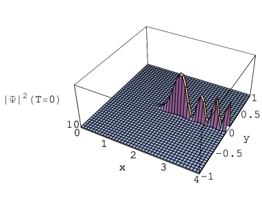
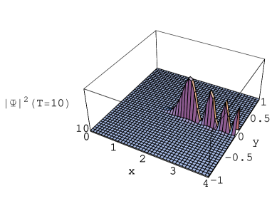
Figure 3: The figures show $|\Psi(x,y,T)|^{2}$, the square of the wavefunction in two different time parameter $T=0,10$. For larger $T$’s the same pattern is repeated. The figures are plotted for the numerical values $\xi=0.1$, $\sigma=\varsigma=10$ and $\nu_{0}=E_{0}=1$, and we have taken the integrals in (83) from $0$ to $15$ for $E$ and from $0$ t0 $4$ for $\nu$.

In figure 3 we have plotted the square of the above wavefunction for some numerical values of the parameters. The figures show that the wavefunction has several peaks which are sharply distributed around $y=0$. Also, it is seen that as time grows, the pattern of the wave packets do not show a major change. This means that in the context of our quadratic model the universe in its radiation era has almost a constant scale factor and thus its scalar curvature vanishes.

Now, let us pursue the corresponding classical cosmology given by the system (39) with $\alpha=1/3$, $V(\phi)=\frac{1}{4}\phi^{2}$ and $k=0$. In figure 4 we have prepared the approximate behavior of $a(t)$, and $\phi(t)\sim R(t)$ for typical values of the parameters and initial conditions respectively. As the figure shows, in complete agreement with the quantum model, the universe follows a zero Ricci scalar while its scale factor has a constant value in the epoch of the radiation dominated era of cosmic evolution.

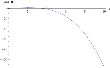
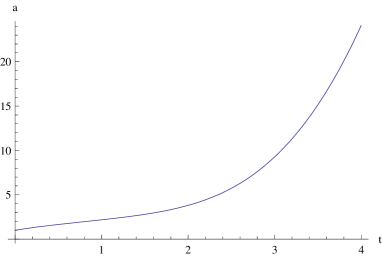
Figure 4: Approximate behavior of $a(t)$, the scale factor and $R(t)$, the Ricci scalar, in the classical cosmology framework. The figures are plotted for numerical values $\alpha=1/3$, $k=0$ and $P_{0}=1$. We take the initial conditions $a(t=0)=1$, $\phi(t=0)=0$, $P_{a}(t=0)=-10$ and $P_{\phi}(t=0)=-1$. After examining some other acceptable sets of initial conditions, we verify that this behavior is almost repeated.

5 Comparison with $f(R)=R$ model

In this section we briefly review the problem in the usual $f(R)=R$ framework which originally appeared in [14]. The Einstein-Hilbert Hamiltonian of the model used in the present work can be written as

$$H=N{\cal H}=N\left(-\frac{P_{a}^{2}}{24a}-6ka+\frac{P_{T}}{a^{3\alpha}}\right).$$ (84)

Therefore, the equations of motion become

$$\left\{\begin{array}[]{ll}\dot{a}=\{a,H\}=-\frac{NP_{a}}{12a},\\ \\ \dot{P_{a}}=\{P_{a},H\}=-N\left(\frac{P_{a}^{2}}{24a^{2}}-6k-3\alpha\frac{P_{T}}{a^{3\alpha+1}}\right),\\ \\ \dot{T}=\{T,H\}=\frac{N}{a^{3\alpha}},\\ \\ \dot{P_{T}}=\{P_{T},H\}=0.\end{array}\right.$$ (92)

Choosing the gauge $N=a^{3\alpha}$, we have $T=t$ and the following constraint equation ${\cal H}=0$

$$-6\frac{\dot{a}^{2}}{a^{3\alpha-1}}-6ka^{3\alpha+1}+P_{0}=0,$$ (93)

where $P_{T}=P_{0}=\mbox{const.}$ as before. For flat space-time ($k=0$), the above equation has the solution

$$a(t)=a_{0}e^{\sqrt{\frac{P_{0}}{6}}t},$$ (94)

for stiff matter ($\alpha=1$), and

$$a(t)=\sqrt{\frac{P_{0}}{6}}t+a_{0},$$ (95)

for radiation ($\alpha=1/3$). It is clear that for both of these solutions the Ricci scalar $R=\frac{6}{N^{2}}\left(\frac{\ddot{a}}{a}+\frac{\dot{a}^{2}}{a^{2}}-\frac{\dot{N}\dot{a}}{Na}\right)$ has a behavior $R\rightarrow 0$ as $t\rightarrow+\infty$. In the case when the universe is filled with stiff matter, comparison of the solution (94) with those of the quadratic model which appear in figure 2, shows that while the scale factors have the same behavior at late times, their early-time evolution does not coincide with each other. This means that although the quadratic model can predict the late time expansion of the universe, but in spite of the usual $f(R)=R$ model its Ricci scalar grows monotonically with time. Also, for radiation the results of two models show some differences. In $f(R)=R$ cosmology the scale factor has a linearly expanding behavior according to (95), with a decreasing Ricci scalar while the quadratic cosmology shows a static universe with zero Ricci scalar. To give an estimate why the result of the quadratic $R^{2}$ -cosmology decline from those of the linear Einstein-Hilbert theory, we should note that although this form of $f(R)$ gravity yields a late time expansion cosmology, but in view of having the correct weak-field limit at Newtonian and post-Newtonian levels has not a desired form. The conditions under which a modified gravity model passes the local and astrophysical tests such as Newton law and solar system tests are investigated in [22]. In these works such $f(R)$ theories are studied which satisfy the conditions

$$\lim_{R\rightarrow\infty}f(R)=\mbox{cons.},\hskip 14.22636pt\lim_{R\rightarrow 0}f(R)=0,$$ (96)

and shown that they pass Newton law, stability of Earth-like gravitational solution, heavy mass for additional scalar degree of freedom, etc. Therefore, since our quadratic model does not satisfy the above conditions, it is not a viable theory with correct Newtonian and post-Newtonian limits. This is not surprising since it is well known that a large class of $f(R)$ theories suffer from this issue [9]. In summary, in the framework of quadratic model, although we have a compatible classical and quantum cosmology discussed in previous sections, the predictions of this model do not coincide with the usual $f(R)=R$ case.

6 Conclusions

In this paper we have studied a quantum cosmological model in the framework of quadratic $f(R)$ gravity coupled to the Schutz’ perfect fluid. The use of Schutz’ formalism for perfect fluid allowed us to obtain a SWD equation in which the only remaining matter degree of freedom plays the role of time parameter in the model. For stiff fluid ($\alpha=1$) and radiation ($\alpha=1/3$), we saw that the SWD equation can be separated and its eigenfunctions can be obtained in terms of known special functions. In the case of stiff matter as the cosmic fluid, we found the eigenstates in terms of Bessel functions and then constructed the corresponding wave packets by appropriate superposition of the eigenstates. The wavefunction in this case shows a pattern in which there are different possible quantum states (with different probability) from which our present universe could have evolved and tunneled in the past from one state to another. The time evolution of this wave packet represents its motion along the larger $R$ direction. We have also solved the corresponding classical cosmology in this case by numerical methods and showed that the Ricci scalar has a monotonically growing behavior with time while the scale factor first decreases and then increases forever. Therefore, we have a model with compatible classical and quantum cosmology which although can predict the late time expansion of the universe, but contrary to the usual standard model of cosmology the universe will admit states with larger $R$ in its late time evolution. On the other hand, in the case of radiation, we obtained wavefunctions which preserve their configuration during time evolution. These wavefunctions peak sharply around the zero Ricci scalar. The classical cosmology in this case is again in agreement with the quantum model and shows an almost static universe with zero scalar curvature. Since in the standard model the universe has an expansion behavior as $a(\eta)\sim\eta^{1/2}$ ($\eta$ is the cosmic time) in its radiation dominated era, our quadratic model does not coincide with real cosmological observations also in this epoch.
Acknowledgements
The author is grateful to the anonymous referees for enlightening suggestions, to H. R. Sepangi for a careful reading of the manuscript and helpful comments and to the research council of Azad University of Chalous for financial support.

References

-
[1]
C. Deffayet, Phys. Lett. B 502 (2001) 199
(arXiv: hep-th/0010186)
J.S. Alcaniz, Phys. Rev. D 65 (2002) 123514 (arXiv: astro-ph/0202492)
S.M. Carroll, V. Duvvuri, M. Trodden and M. Turner, Phys. Rev. D 70 (2004) 043528 (arXiv: astro-ph/0306438)
S. Nojiri and S.D. Odintsov, Phys. Lett. B 576 (2003) 5 (arXiv: hep-th/0307071)
K. Atazadeh and H.R. Sepangi, Int. J. Mod. Phys. D 16 (2007) 687 (arXiv: gr-qc/0602028)
S. Nojiri, S.D. Odintsov and M. Sami, Phys. Rev. D 74 (2006) 046004 (arXiv: hep-th/0605039)
S. Capozziello and M. Francaviglia, Gen. Rel. Grav. 40 (2008) 357 (arXiv: 0706.1146 [gr-qc])
S. Capozziello, Int. J. Mod. Phys. D 11 (2002) 483 (arXiv: gr-qc/0201033)
S. Nojiri and S. D. Odintsov, Phys.Rev. D 68 (2003) 123512 (arXiv:hep-th/0307288)
S.K. Chakrabarti, E.N. Saridakis and A.A. Sen, A new approach to modified-gravity models (arXiv: 0908.0293 [astro-ph.CO]) -
[2]
S. Nojiri and S.D. Odintsov, Dark energy, inflation and dark matter from modified
gravity (arXiv: 0807.0685 [hep-th])
S. Nojiri and S.D. Odintsov, Int. J. Geom. Methods Mod. Phys. 4 (2007) 115 (arXiv: hep-th/ 0601213)
T.P. Sotiriou and V. Faraoni, theories of gravity (arXiv: 0805.1726 [gr-qc]) - [3] D. Lovelock, J. Math. Phys. 12 (1971) 498
- [4] K.S. Stelle, Phys. Rev. D 16 (1977) 953
- [5] R. Utiyama and B. DeWitt, J. Math. Phys. 3 (1962) 608
-
[6]
K.S. Stelle, Gen. Rel. Grav. 9 (1978) 353
G.T. Horowitz and R.M. Wald, Phys. Rev. D 17 (1978) 414 - [7] K. Kleidis, A. Kuiroukidis and D.B. Papadopoulos, Phys. Lett. B 546 (2002) 112
-
[8]
D.N. Vollick, Phys. Rev. D 68 (2003)
063510 (arXiv: astro-ph/0306630)
X. Meng and P. Wang, Class. Quantum Grav. 20 (2003) 4949 (arXiv: astro-ph/0307354)
X. Meng and P. Wang, Palatini formulation of modified gravity with squared scalar curvature (arXiv: astro-ph/0308284)
X. Meng and P. Wang, Phys. Lett. B 584 (2004) 1 (arXiv: hep-th/0309062) -
[9]
T. Chiba, Phy. Lett. B 575 (2003) 1 (arXiv: astro-ph/0307338)
E.E. Flanagan, Class. Quantum Grav. 21 (2004) 3817 (arXiv: gr-qc/0403063)
T.P. Sotiriou, Class. Quantum Grav. 23 (2006) 5117 (arXiv: gr-qc/0604028) -
[10]
T.P. Sotiriou and S. Liberati, Ann. Phys. 322 (2007) 935 (arXiv: gr-qc/0604006)
N.J. Poplawski, Class. Quantum Grav. 23 (2006) 2011 (arXiv: gr-qc/0510007) -
[11]
M.C.B. Abdalla, A. Nojiri and S.D. Odintsov, Class. Quantum Grav. 22 (2005) L35 (arXiv: hep-th/0409177)
X. Meng and P. Wang,Class. Quantum Grav. 22 (2005) 23 ( arXiv: gr-qc/0411007)
X. Meng and P. Wang, Class. Quantum Grav. 21 (2004) 951 (arXiv: astro-ph/0308031)
T. Clifton and J.D. Barrow, Phys. Rev. D 72 (2005) 103005 (arXiv: gr-qc/0509059)
T. Clifton, Class. Quantum Grav. 23 (2006) 7445 ( arXiv: gr-qc/0607096)
K. Atazadeh and H.R. Sepangi, Phys. Lett. B 643 (2006) 76 (arXiv: gr-qc/0610107)
J.D. Barrow and T. Clifton, Class.Quantum Grav. 23 (2006) L1 ( arXiv: gr-qc/0509085)
B. Vakili, Phys. Lett. B 664 (2008) 16 (arXiv: 0804.3449 [gr-qc])
K. Atazadeh, M. Farhoudi and H.R. Sepangi, Phys. Lett. B 660 (2008) 275 (arXiv: 0801.1398 [gr-qc]) -
[12]
A. Shojai and F. Shojai, Gen. Rel. Grav. 40 (2008) 1967 (arXiv: 0801.3496 [gr-qc])
B. Vakili, Phys. Lett. B 669 (2008) 206 (arXiv: 0809.4591 [gr-qc])
G. Cognola, E. Elizalde, S. Nojiri, S.D. Odintsov and S. Zerbini, J. Cosmol. Astropart. Phys. 0502 (2005) 010 (arXiv: hep-th/0501096)
A.K. Sanyal and B. Modak, Phys. Rev. D 63 (2001) 064021 (arXiv: gr-qc/0107001)
A.K. Sanyal and B. Modak, Class.Quantum Grav. 19 (2002) 515 (arXiv: gr-qc/0107070)
M. Kenmoku, K. Otsuki, K. Shigemoto and K. Uehara, Class. Quantum Grav. 13 (1996) 1751 (arXiv: gr-qc/9510027)
U. Kasper, Class. Quantum Grav. 10 (1993) 869
L.O. Pimentel, O. Obregon and J.J. Rosales, Class. Quantum Grav. 14 (1997) 379
L.O. Pimentel and O. Obregon, Class. Quantum Grav. 11 (1994) 2219 -
[13]
B.F. Schutz, Phys. Rev. D 2 (1970) 2762
B.F. Schutz, Phys. Rev. D 4 (1971) 3559 -
[14]
A.B. Batista, J.C. Fabris, S.V.B. Goncalves and J. Tossa, Phys. Lett. A 283 (2001) 62
(arXiv: gr-qc/0011102)
F.G. Alvarenga, J.C. Fabris, N.A. Lemos and G.A. Monerat, Gen. Rel. Grav. 34 (2002) 651 (arXiv: gr-qc/0106051)
A.B. Batista, J.C. Fabris, S.V.B. Goncalves and J. Tossa, Phys. Rev. D 65 (2002) 063519 (arXiv: gr-qc/0108053)
N.A. Lemos, J. Math. Phys. 37 (1996) 1449 (arXiv: gr-qc/9511082)
P. Pedram, S. Jalalzadeh and S.S. Gousheh, Class. Quantum Grav. 24 (2007) 5515 (arXiv: 0709.1620 [gr-qc])
P. Pedram and S. Jalalzadeh, Phys. Rev. D 77 (2008) 123529 (arXiv: 0805.4099 [gr-qc]) - [15] B.S. DeWitt, Phys. Rev. 160 (1967) 1113
- [16] V.G. Lapchinskii and V.A. Rubakov, Theor. Math. Phys. 33 (1977) 1076
- [17] A. Anderson, Ann. Phys. 232 (1994) 292 (arXiv: hep-th/9305054)
- [18] S.W. Hawking and D.N. Page, Nucl. Phys. B 264 (1986) 185
- [19] R. Steigl and F. Hinterleitner, Class. Quantum Grav. 23 (2006) 3879
- [20] M. Abramowitz and I.A. Stegun, Handbook of Mathematical Functions (1972) (New York: Dover)
-
[21]
C.J. Isham, Canonical quantum gravity and the problem of time (arXiv: gr-qc/9210011)
B. Vakili and H.R. Sepangi, Ann. Phys. 323 (2008) 548 (arXiv: 0709.2988 [gr-qc]) -
[22]
W. Hu and I. Sawicki, Phys. Rev. D 76 (2007) 064004
(arXiv: 0705.1158 [astro-ph])
S. Nojiri and S.D. Odintsov, Newton law corrections and instabilities in gravity with the effective cosmological constant epoch (arXiv: 0706.1378 [hep-th])
S. Nojiri and S.D. Odintsov, Phys. Rev. D 77 (2008) 026007 (arXiv: 0710.1738 [hep-th])