Effect of Thermoelectric Cooling in Nanoscale Junctions

Abstract

We propose a thermoelectric cooling device based on an atomic-sized junction. Using first-principles approaches, we investigate the working conditions and the coefficient of performance (COP) of an atomic-scale electronic refrigerator where the effects of phonon’s thermal current and local heating are included. It is observed that the functioning of the thermoelectric nano-refrigerator is restricted to a narrow range of driving voltages. Compared with the bulk thermoelectric system with the overwhelmingly irreversible Joule heating, the 4-Al atomic refrigerator has a higher efficiency than a bulk thermoelectric refrigerator with the same $ZT$ due to suppressed local heating via the quasi-ballistic electron transport and small driving voltages. Quantum nature due to the size minimization offered by atomic-level control of properties facilitates electron cooling beyond the expectation of the conventional thermoelectric device theory.

I Introduction

The miniaturization of devices has been eliciting a tremendous wave of multidisciplinary scientific interest Aviram ; book . This interest is motivated by the aspiration to develop new forms of electronic devices based on nano-structures. To develop the nano-devices at the atomic/molecular level, understanding of non-equilibrium quantum transport theory is of critical importance. In the past decade, a growing number of studies have been conducted to diversify the scopes of molecular electronics including the current-voltage characteristics Kaun ; DiVentra2 ; Nitzan1 ; Venkataraman ; Gemma , inelastic electron tunneling spectroscopy (IETS) Wang2 ; Ratner3 ; Yluo ; Kushmerick ; Brandbyge ; Dicarlo ; cheniets ; chenh2 ; thygesen , shot noise Ruitenbeek1 ; Kiguchi ; Natelson ; chenshot , counting statistics liushot , local heating chenheating ; Huang2 , and gate-controlled effect DiVentragate ; Ma ; Solomon1 ; Solomon2 ; Reed . Substantial progress has been achieved in experiments and theories Ahn ; Lindsay ; Tao1 .

Recently, atomic/molecular thermoelectric junctions are gaining increased attention due to the recent measurements of the Seebeck coefficient, defined as $S=dV/dT$, $dV$ is the voltage difference caused by the temperature difference $dT$ by the Seebeck effect Ruitenbeek ; Majumdar1 ; Majumdar2 ; Majumdar3 . Measurements of Seebeck coefficient provide a useful experimental approach to exploring the electronic structure of the molecule bridging the electrodes Malen . Methodologically, the scope of the research needs to extend through the utilization of unprecedented experiments. These experiments inspire rapid development in the theory of thermoelectricity at the atomic and molecular scale including the Seebeck coefficients, thermoelectric figure of merit ($ZT$), thermospin effect, and effect of electron-phonon interactions Paulsson ; Zheng ; Wang ; Pauly ; Galperin ; Dubi ; Markussen ; Ke ; Finch ; Troels ; Segal ; Bergfield ; Liu ; Liu2 ; Hsu .

Effect of thermoelectricity hybridizes the interactions between electron and energy transport under non-equilibrium conditions. In the bulk and mesoscopic systems, the efficiency of a thermoelectric (TE) refrigerator is usually suppressed by a large work function. For example, the operation of a thermoelectric cooling device such as a vacuum diode is limited to very high temperatures ($T_{op}>1000$ K) due to its large potential barrier Mahan1 . Another pronounced drawback in the bulk system is the overwhelmingly irreversible Joule heating due to diffused electrons which significantly suppresses the efficiency of thermoelectric refrigerators. Recently, researchers have looked into creating thermoelectric refrigerators that operate at room temperatures. For this purpose, semiconductor hetero-structures have been proposed to reduce the work function Mahan2 ; Chao ; Dwyer ; Westover . A new solution to the low temperature-operated thermoelectric refrigerators may be the atomic-sized junctions, the extreme limit of device miniaturization.

The atomic-sized energy-conversion devices have gained growing interest in material science and nanoscience. The electron transport mechanism in theses systems is characterized by quasi-ballistic electron transport due to the small size. Previous reports thus far have mainly focused on the Seebeck coefficient ($S$) and the thermoelectric figure of merit ($ZT$) of nanojunctions. Several attempts have been made to understand the cooling mechanism in nanojunctions DiventraS ; Galperin2 ; Segalreg1 ; Segalreg2 . This study proposes a thermoelectric cooling device based on an atomic junctions. This project develops a theory of the atomic-scale cooling mechanism for quasi-ballistic electrons under non-equilibrium conditions from first-principles approaches. We investigate the nano-refrigerator’s working conditions, the electron’s thermal current which removes heat from the cold temperature reservoir, and the coefficient of performance (COP) in the presence of the phonon’s thermal current and local heating. We observe that the potential barrier is effectively suppressed by the resonant tunneling and the local heating is significantly suppressed by the reduced dimension. Nano-refrigerators with a figure of merit comparable to conventional TE refrigerators usually have better coefficient of performance, taking advantage the reduced local heating due to the small size. These quantum features remarkably facilitates the electron cooling in nanoscale thermoelectric refrigerators beyond the expectation of the conventional bulk thermoelectric device theory.

As an example, we consider an ideal 4-Al monatomic junction, as depicted in Fig. 1(a). The 4-Al atomic junction is marked by a larger Seebeck coefficient induced by a sigma channel near the chemical potentials with the $P_{x}-P_{y}$ orbital characters. Due to the small size, local heating and photon radiation are sufficiently suppressed that they can be safely neglected compared with the large phonon’s thermal current considered in this study. Calculations indicate that the 4-Al junction is able to work at temperatures below 100 K. Compared with atomic-scale thermoelectric power generators liupowergen ; Justin , thermoelectric nano-refrigerators require more stringent working conditions. For example, we observe that the battery which drives thermoelectric nano-refrigerator is restricted to a range of voltages between the lower and upper threshold biases.

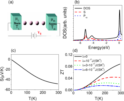
Figure 1: (color online) (a) Scheme of the 4-Al atomic junction with different temperatures $T_{L(R)}$ and chemical potentials $\mu_{L(R)}$. The Al-jellium distance is about $2.5$ a.u. and the Al-Al bond distance is about $6.3$ a.u.; (b) Density of state and projected density of states of the 4-Al junction; (c) Seebeck coefficient vs. temperature of the 4-Al junction; and (d) $ZT$ vs. T with the phonon’s thermal current for various values of $\lambda$.

The flow of the discussion in this paper is as follows. Firstly, in Sec. II. we describe the details of density functional theory, theory of thermoelectricity, and theory of thermoelectric nano-refrigerator without and with the phonon’s thermal current and local heating. In Sec. III., we discuss the thermoelectric properties of 4-Al atomic junctions, and subsequently discuss the onset bias, working conditions, and COP of thermoelectric nano-refrigerators. We then summarize our findings in Sec. IV.

II Theoretical Methods

The theory presented in the following is general to any atomic/molecular junction characterized by the quasi-ballistic transport. In Sec. II.  A., we present an introduction of the density-functional theory (DFT). In Sec. II. B., we present the theory to calculate the Seebeck coefficient, electric conductance, electron’s thermal conductance, phonon’s thermal conductance, and thermoelectric figure of merit ($ZT$). In Sec. II. C., we present the theory for electronic cooling without and with the phonon’s thermal current and local heating.

II.1 Density Functional Theory

We present a brief introduction of how to calculate the electric current and the electron’s thermal current in the DFT framework. We picture a nanoscale junction as formed by two semi-infinite electrodes held apart at a fixed distance with a nano-structured object bridging the gap between them. The full Hamiltonian of the system is $H=H_{0}+V$, wherein $H_{0}$ is the Hamiltonian due to the bare electrodes and $V$ is the scattering potential of the nano-structured object.

First, we calculate the wave functions of the bare electrodes with an applied bias $V_{B}=(\mu_{R}-\mu_{L})/e$, where $\mu_{L(R)}$ is the chemical potential deep in the left (right) electrode. The unperturbed wave functions of the bare electrodes have the form, $\Psi_{E\mathbf{K}_{\parallel}}^{0,L(R)}(\mathbf{r})=e^{i\mathbf{K}_{\parallel}\mathbf{\cdot R}}\cdot u_{E\mathbf{K}_{\parallel}}^{L(R)}(z)$, where $u_{E\mathbf{K}_{\parallel}}^{L(R)}(z)$ describes the electrons incident from the left (right) electrode before the inclusion of the nano-structured object. The wavefunction $u_{E\mathbf{K}_{\parallel}}^{L(R)}(z)$ is calculated by solving the Shrödinger equation and Poisson equations iteratively until self-consistency is obtained. Note that $u_{E\mathbf{K}_{\parallel}}^{R}(z)$ satisfies the following boundary condition:

$$u_{E\mathbf{K}_{\parallel}}^{R}(z)=(2\pi)^{-\frac{3}{2}}\times\genfrac{\{}{.}{0.0pt}{}{\frac{1}{\sqrt{k_{R}}}(e^{-ik_{R}z}+R\text{ }e^{ik_{R}z}),\text{ }z\rightarrow\infty,}{\frac{1}{\sqrt{k_{L}}}T\text{ }e^{-ik_{L}z},\text{ }z\rightarrow-\infty,}$$ (1)

where $\mathbf{K}_{\parallel}$ is the electron momentum in the plane parallel to the electrode surfaces, and $z$ is the coordinate parallel to the direction of the current. The condition of energy conservation gives $\frac{1}{2}k_{R}^{2}=E-\frac{1}{2}\left|\mathbf{K}_{\parallel}\right|^{2}-v_{eff}(\infty)$ and $\frac{1}{2}k_{L}^{2}=E-\frac{1}{2}\left|\mathbf{K}_{\parallel}\right|^{2}-v_{eff}(-\infty)$, where $v_{eff}(z)$ is the effective potential comprising the electrostatic and exchange-correlation potentials.

The nano-structured object is considered as a scattering center. The scattering wave functions of the entire system are calculated by solving the Lippmann-Schwinger equation in the scattering approaches iteratively until self-consistency is obtained,

$$\Psi_{E\mathbf{K}_{\parallel}}^{L(R)}(\mathbf{r})=\Psi_{E\mathbf{K}_{\parallel}}^{0,L(R)}(\mathbf{r})+\int d^{3}\mathbf{r}_{1}\int d^{3}\mathbf{r}_{2}G_{E}^{0}(\mathbf{r},\mathbf{r}_{1})V(\mathbf{r}_{1},\mathbf{r}_{2})\Psi_{E\mathbf{K}_{\parallel}}^{L(R)}(\mathbf{r}_{2}),$$ (2)

where $\Psi_{E\mathbf{K}_{\parallel}}^{L(R)}(\mathbf{r})$ stands for the effective single-particle wave functions of the entire system, which also represents the electrons with energy $E$ incident from the left (right) electrode. The potential $V(\mathbf{r}_{1},\mathbf{r}_{2})$ that the electrons experience when they scatter through the nanojunction is

$$V(\mathbf{r}_{1},\mathbf{r}_{2})=V_{ps}(\mathbf{r}_{1},\mathbf{r}_{2})+\left\{\left(V_{xc}\left[n\left(\mathbf{r}_{1}\right)\right]-V_{xc}\left[n_{0}\left(\mathbf{r}_{1}\right)\right]\right)+\int d\mathbf{r}_{3}\frac{\delta n\left(\mathbf{r}_{3}\right)}{\left|\mathbf{r}_{1}-\mathbf{r}_{3}\right|}\right\}\delta(\mathbf{r}_{1}-\mathbf{r}_{2}),$$ (3)

where $V_{ps}(\mathbf{r}_{1},\mathbf{r}_{2})$ is the electron-ion interaction potential represented with pseudopotential; $V_{xc}\left[n\left(\mathbf{r}\right)\right]$ is the exchange-correlation potential calculated at the level of the local-density approximation; $n_{0}\left(\mathbf{r}\right)$ is the electron density for the pair of biased bare electrodes; $n\left(\mathbf{r}\right)$ is the electron density for the total system; and $\delta n\left(\mathbf{r}\right)$ is their difference. The quantity $G_{E}^{0}$ is the Green’s function for the bare electrodes. The wavefunctions that achieve self-consistency in the DFT framework in plane wave basis are applied to calculate the electric current, and the electron’s thermal current.

These right- and left-moving wave functions weighed with the Fermi-Dirac distribution function according to their energies and temperatures are applied to calculate the electric current as

$$I(\mu_{L},T_{L};\mu_{R},T_{R})=\frac{e\hbar}{mi}\int dE\int d\mathbf{r}_{\mathbf{\perp}}\int d\mathbf{K}_{\parallel}\left[f_{E}(\mu_{R},T_{R})I_{E{E},\mathrm{\mathbf{K}}_{||}}^{RR}(\mathbf{r})-f_{E}(\mu_{L},T_{L})I_{E{E},\mathrm{\mathbf{K}}_{||}}^{LL}(\mathbf{r})\right],$$ (4)

where $I_{E{E}^{\prime},\mathrm{\mathbf{K}}_{||}}^{RR(LL)}(\mathbf{r})=\left[\Psi_{E,\mathrm{\mathbf{K}}_{||}}^{R(L)}(\mathbf{r})\right]^{\ast}\nabla\Psi_{{E}^{\prime},\mathrm{\mathbf{K}}_{||}}^{R(L)}(\mathbf{r})-\nabla\left[\Psi_{E,\mathrm{\mathbf{K}}_{||}}^{R(L)}(\mathbf{r})\right]^{\ast}\Psi_{{E}^{\prime},\mathrm{\mathbf{K}}_{||}}^{R(L)}(\mathbf{r})$ and $d\mathbf{r}_{\mathbf{\perp}}$ represents an element of the electrode surface. Here, we assume that the left and right electrodes are independent electron reservoirs, with the population of the electron described by the Fermi-Dirac distribution function, $f_{E}(\mu_{L(R)},T_{L(R)})=1/\{\exp[\left(E-\mu_{L(R)}\right)/(k_{B}T_{L(R)})]+1\}$, where $\mu_{L(R)}$ and $T_{L(R)}$ are the chemical potential and the temperature in the left (right) electrode, respectively. More detailed descriptions of theory can be found in Refs. [63; 4; 64].

The above expression can be cast in a Landauer-Büttiker formalism:

$$I(\mu_{L},T_{L};\mu_{R},T_{R})=\frac{2e}{h}\int dE\tau(E)[f_{E}(\mu_{R},T_{R})-f_{E}(\mu_{L},T_{L})],$$ (5)

where $\tau(E)=\tau^{R}(E)=\tau^{L}(E)$ is a direct consequence of the time-reversal symmetry, and $\tau^{R(L)}(E)$ is the transmission function of the electrons with energy $E$ incident from the right (left) electrode,

$$\tau^{R(L)}(E)=\frac{\pi\hbar^{2}}{mi}\int{d\mathbf{r}}_{\perp}{\int{d\mathrm{\mathbf{K}}_{||}}}I_{EE,\mathrm{\mathbf{K}}_{||}}^{RR(LL)}(\mathrm{\mathbf{r}}).$$ (6)

There is an analog between the electric current and electron’s thermal current. The flow of electrons can also transport energy. The electron’s thermal current, defined as the rate at which thermal energy flows from the right (into the left) electrode, is

$$J_{el}^{R(L)}(\mu_{L},T_{L};\mu_{R},T_{R})=\frac{2}{h}\int dE(E-\mu_{R(L)})\tau(E)[f_{E}(\mu_{R},T_{R})-f_{E}(\mu_{L},T_{L})].$$ (7)

II.2 Theory of Thermoelectricity

Here, we present the theory to calculate the zero-bias electric conductance, Seebeck coefficient, and electron’s thermal conductance for a thermoelectric nanojunction in terms of the effective single-particle wave-functions obtained self-consistently within the static density-functional theory in a truly atomic-scale junction.

We assume that the left and right electrodes serve as independent temperature reservoirs. The population of electrons in the left (right) electrode is described by the Fermi-Dirac distribution function, $f_{E}(\mu_{L(R)},T_{L(R)})=1/\{\exp[\left(E-\mu_{L(R)}\right)/(k_{B}T_{L(R)})]+1\}$, where the chemical potentials are $\mu_{R}=\mu_{L}=\mu$ (i.e., at zero external bias). Let us now consider an extra infinitesimal current induced by an additional infinitesimal temperature ($dT$) and voltage ($dV$) across the junctions in a open circuit. The current induced by $dT$ and $dV$ are $(dI)_{T}=I(\mu,T;\mu,T+dT)$ and $(dI)_{V}=I(\mu,T;\mu+edV,T)$, respectively, where $I(\mu,T;\mu,T+dT)$ and $I(\mu,T;\mu+edV,T)$ are given by Eq. (5). Suppose that the current cannot actually flow in an open circuit, thus, $(dI)_{T}$ counterbalances $(dI)_{V}$. In other words, the extra net current is zero,

$$dI=I(\mu,T;\mu+edV,T+dT)\approx(dI)_{T}+(dI)_{V}=0.\text{ }$$ (8)

The Fermi-Dirac distribution function in Eq. (8) can be expanded up to the first order in $dT$ and $dV$, and we obtain the Seebeck coefficient (defined by $S=dV/dT$),

$$S(\mu,T)=-\frac{1}{eT}\frac{K_{1}(\mu,T)}{K_{0}(\mu,T)},$$ (9)

where

$$K_{n}(\mu,T)=-\int dE\tau(E)\left(E-\mu\right)^{n}\frac{\partial f_{E}(\mu,T)}{\partial E}.$$ (10)

The Seebeck coefficient in the low-temperature regime can be obtained by expanding $K_{n}(\mu,T)$ to the lowest order in temperatures through the Sommerfeld expansion, that is, $K_{0}\approx\tau(\mu)$, $K_{1}\approx[\pi^{2}k_{B}^{2}\tau^{\prime}(\mu)/3]T^{2}$, and $K_{2}\approx[\pi^{2}k_{B}^{2}\tau(\mu)/3]T^{2}$. The Seebeck coefficient up to the lowest order in temperature is

$$S\approx\alpha T,$$ (11)

where $\alpha=-\pi^{2}k_{B}^{2}\frac{\partial\tau(\mu)}{\partial E}/\left(3e\tau(\mu)\right)$. The Seebeck coefficient is positive (negative) when the slope of transmission function is negative (positive), which is closely related to the transmission function near the chemical potentials.

The electron’s thermal current is the energy current carried by electrons traveling between electrodes driven by $dT$ and $dV$. Analogous to the extra current given by Eq. (8), the extra electron’s thermal current is

$$dJ_{el}=(dJ_{el})_{T}+(dJ_{el})_{V}.$$ (12)

where $(dJ_{el})_{T}=J_{el}(\mu,T;\mu,T+dT)$ and $(dJ_{el})_{V}=J_{el}(\mu,T;\mu+edV,T)$ are the fractions of electron’s thermal current driven by $dT$ and $dV$, respectively. Note that $dV$ is generated by the Seebeck effect according to the temperature difference $dT$. Both $J_{el}(\mu,T;\mu,T+dT)$ and $J_{el}(\mu,T;\mu+edV,T)$ can be calculated using Eq. (7).

Given that we define the electron’s thermal conductance as $k_{el}=dJ_{el}/dT$, the electron’s thermal conductance $k_{el}$ can decomposed into two components:

$$\kappa_{el}(\mu,T)=\kappa_{el}^{T}(\mu,T)+\kappa_{el}^{V}(\mu,T),$$ (13)

where $\kappa_{el}^{T}=(dJ_{el})_{T}/dT$ and $\kappa_{el}^{V}=(dJ_{el})_{V}/dT$. We note that $\kappa_{el}^{T}$ and $\kappa_{el}^{V}$ are the portions of the electron’s thermal conductance driven by $dT$ and $dV$, respectively. Analogous to Eq. (9), $\kappa_{el}^{T}$ and $\kappa_{el}^{V}$ can be can be expressed by Eq. (10):

$$\kappa_{el}^{T}(\mu,T)=\frac{2}{h}\frac{K_{2}(\mu,T)}{T},$$ (14)

and

$$\kappa_{el}^{V}(\mu,T)=\frac{2e}{h}K_{1}(\mu,T)S(\mu,T).$$ (15)

One should note that $\kappa_{el}^{V}=0$ if the Seebeck coefficient of the system is zero because $dV$ is zero.

In the low-temperature regime, $\kappa_{el}^{T}$ and $\kappa_{el}^{V}$ can be expanded to the lowest order in temperatures using the Sommerfeld expansion:

$$\kappa_{el}^{V}\approx\beta_{V}T\text{ }^{3}\text{and }\kappa_{el}^{T}\approx\beta_{T}T,$$ (16)

where $\beta_{V}=-2\pi^{4}k_{B}^{4}[\tau^{\prime}(\mu)]^{2}/(9h\tau(\mu))$ and $\beta_{T}=2\pi^{2}k_{B}^{2}\tau(\mu)/(3h)$. In the above expansions, we also applied the following approximations: $K_{1}(\mu,T)\approx[\pi^{2}k_{B}^{2}\tau^{\prime}(\mu)/3]T^{2}$, $K_{2}(\mu,T)\approx[\pi^{2}k_{B}^{2}\tau(\mu)/3]T^{2}$, and Eq. (11). In the low-temperature regime, $\kappa_{el}^{T}$ dominates the electron’s thermal current. Thus $\kappa_{el}\approx\kappa_{el}^{T}$ is linear in T, that is,

$$\kappa_{el}(\mu,T)\approx\beta_{T}T.$$ (17)

At zero bias, the electric conductance can be expressed as

$$\sigma(T)=\frac{2e^{2}}{h}\int dEf_{E}\left(\mu,T\right)[1-f_{E}\left(\mu,T\right)]\tau(E)/(k_{B}T).$$ (18)

In the low-temperature regime, the zero-bias conductance is usually insensitive to temperatures if tunneling is the major transport mechanism.

Thus far, the physical quantities ($S$, $\sigma$, and $\kappa_{el}$) previously discussed are related to the propagation of electrons. The heat current carried by phonon may occur in a real system. The phonon’s thermal current, which is driven by the temperature difference $\Delta T,$ flows from the hot reservoir into the cold reservoir. To determine the impact of the phonon’s thermal current on refrigeration, the weak link model is chosen to describe it. The weak link model assumes that the nanojunction is a weak elastic link with a given stiffness $K$ that can be evaluated from total energy calculations or from experimental measurement Patton . Two metal electrodes are regarded as the macroscopic bodies under their thermodynamic equilibrium, and are taken as ideal thermal conductors. To the leading order in the strength of the weak link, the phonon’s thermal current ($J_{ph}$) via elastic phonon scattering is Patton ,

$$J_{ph}=\frac{2\pi K^{2}}{\hbar}\int_{0}^{\infty}dEEN_{L}(E)N_{R}(E)[n_{L}(E)-n_{R}(E)],$$ (19)

where $K$ is the stiffness of the weak elastic link; $N_{L(R)}(E)$ is the spectral density of phonon states at the left (right) electrode surface which is measurable by experiments; and $n_{L(R)}\equiv 1/(e^{E/K_{B}T_{L(R)}}-1)$ is the Bose-Einstein distribution function. In the long wave length limit, the spectral density of surface phonon is given by $N_{L(R)}(E)\approx CE$. The phonon’s thermal conductance defined as $\kappa_{ph}=\Delta J_{ph}/\Delta T$ as $\Delta T\rightarrow 0$, is

$$\kappa_{ph}=[J_{ph}(T_{L}+\frac{\Delta T}{2},T_{R}-\frac{\Delta T}{2})-J_{ph}(T_{L},T_{R})]/\Delta T.$$ (20)

Expanding the Bose-Einstein distribution function in $J_{ph}(T_{L}+\frac{\Delta T}{2},T_{R}-\frac{\Delta T}{2})$ to the first order of $\Delta T$, we obtain the phonon’s thermal conductance:

$$\kappa_{ph}=\frac{\pi K^{2}C^{2}}{\hbar}\int_{0}^{\infty}dEE^{3}\sum_{i=L,R}\frac{\partial n_{i}(E)}{\partial T_{i}}.$$ (21)

When $T_{R}\approx T_{L}=T$, then Eq. (21) is reduced to,

$$\kappa_{ph}=\frac{2\pi K^{2}C^{2}}{\hbar}\int_{0}^{\infty}dEE^{3}\frac{\partial n(E)}{\partial T}.$$ (22)

where $n=1/[e^{E/(k_{B}T)}-1]$.

The efficiency of thermoelectric nano-devices is conventionally described by the thermoelectric figure of merit $ZT$, which depends on the following physical factors: Seebeck coefficient $(S)$, electric conductance $(\sigma)$, electron’s thermal conductance $(\kappa_{el})$, and phonon’s thermal conductance $(\kappa_{ph})$. $ZT$ is defined as

$$ZT=\frac{S^{2}\sigma}{\kappa_{el}+\kappa_{ph}}T,$$ (23)

where $S$, $\sigma$, $\kappa_{el}$, and $\kappa_{ph}$ can be numerically calculated using Eqs. (9), (18), (13), and (22), respectively. When $ZT$ tends to infinity, the thermoelectric efficiency of nanojunctions will reach Carnot efficiency.

II.3 Theory of Thermoelectric Refrigerator

Now, we present the theory of thermoelectric cooling device at atomic scale including effect of the phonon’s thermal current and local heating. We assume that the left (right) electrode serves as the hot (cold) temperature reservoir with temperature $T_{R}=T_{C}$ ($T_{L}=T_{H}=T_{C}+\Delta T$) and the phonon’s population is described by Bose-Einstein distribution function. We consider the nanojunction connecting to an external battery with bias $V_{B}=(\mu_{R}-\mu_{L})/e$, which drives the electrons flowing from the right- to left-electrodes. The thermal current carried by electrons traveling between two electrodes is given by Eq. (7). It should be noted that

$$J_{el}^{R}(\mu_{L},T_{L};\mu_{R},T_{R})+I(\mu_{L},T_{L};\mu_{R},T_{R})V_{B}=J_{el}^{L}(\mu_{L},T_{L};\mu_{R},T_{R}),$$ (24)

which $I(\mu_{L},T_{L};\mu_{R},T_{R})$ is the current given by Eq. (5). Equation (24) states that the energy is conserved: it consumes electric energy to take heat from the right (cold) into left (hot) reservoir. Thus, the thermoelectric junction can be regarded as an electronic cooling device when $J_{el}^{R}>0$, which states that the thermoelectric junction is capable of removing heat from the cold reservoir.

A measure of a refrigerator’s performance is the ratio of the rate of heat removed from the cold reservoir to the electric power done on the system. The ratio is called the coefficient of performance (COP):

$$\eta_{el}=\frac{J_{el}^{R}}{IV_{B}}=\frac{J_{el}^{R}}{\left|J_{el}^{R}-J_{el}^{L}\right|},$$ (25)

where $V_{B}$ is the bias applied across the nanojunction driving the thermoelectric refrigerator, $I$ is the electric current, and $J_{el}^{R}$ is the rate of thermal energy removed from the cold reservoir. The thermoelectric junction as a nano-refrigerator is working when $J_{el}^{R}>0$ (and thus $\eta_{el}>0$).

II.3.1 Properties of Thermoelectric Refrigerator in the Absence of the Phonon’s Thermal Current

In the following, we develop an analytical theory to gain insight into the fundamentals of the cooling effect in the thermoelectric nanojunction. We apply the Sommerfeld expansion to $J_{el}^{R}(\mu_{L},T_{L};\mu_{R},T_{R})$ and obtain,

$$J_{el}^{R} \approx\frac{\pi^{2}k_{B}^{2}}{3h}\left[\tau(\mu_{L})(T_{R}^{2}-T_{L}^{2})+\tau^{\prime}(\mu_{L})(\mu_{R}-\mu_{L})(T_{R}^{2}+T_{L}^{2})\right]$$

$$-\frac{1}{h}\left[\tau(\mu_{L})(\mu_{R}-\mu_{L})^{2}\right]-\frac{1}{3h}\left[\tau^{\prime}(\mu_{L})(\mu_{R}-\mu_{L})^{3}\right],$$ (26)

where we use the following relations: $\tau(E)\approx$ $\tau(\mu_{L})+\tau^{\prime}(\mu_{L})(E-\mu_{L})$, $\tau(\mu_{R})\approx$ $\tau(\mu_{L})+\tau^{\prime}(\mu_{L})(\mu_{R}-\mu_{L})$, $T_{L}=T_{R}+\Delta T$, $\int_{\mu_{L}}^{\mu_{R}}(E-\mu_{R})dE=-\frac{1}{2}(\mu_{R}-\mu_{L})^{2}$, $\int_{\mu_{L}}^{\mu_{R}}(E-\mu_{L})(E-\mu_{R})dE=-\frac{1}{6}(\mu_{R}-\mu_{L})^{3}$, and $\mu_{R}-\mu_{L}=eV_{B}$. When $\Delta T\ll T_{R}$, Eq. (26) can be expressed as a polynomial of $V_{B}$:

$$J_{el}^{R}=-a+bV_{B}-cV_{B}^{2}-dV_{B}^{3},$$ (27)

where $a=2\pi^{2}k_{B}^{2}\tau(\mu)T_{R}\Delta T/(3h)$, $b=2e\pi^{2}k_{B}^{2}\tau^{\prime}(\mu)T_{R}^{2}/(3h)$, $c=e^{2}\tau(\mu)/h$, and $d=e^{3}\tau^{\prime}(\mu)/(3h)$. The above equation is convenient for analytical exploration of the properties of thermoelectric nano-refrigerators.

A thermoelectric nano-refrigerator functions only when the maximum value of the electron’s thermal current is positive, that is, $\left(J_{el}^{R}\right)_{\max}>0$. In a small bias regime, the term $V_{B}^{3}$ can be neglected in Eq. (27), i.e., $J_{el}^{R}\approx-a+bV_{B}-cV_{B}^{2}$. In this case, the working condition of nano-refrigerator is given by $\left(J_{el}^{R}\right)_{\max}=(-4ac+b^{2})/(4c)>0$, which yields the criterion for the existence of electronic cooling

$$-S>\sqrt{\frac{2\pi^{2}k_{B}^{2}}{3e^{2}}\left(\frac{\Delta T}{T_{R}}\right)},$$ (28)

where $S=-\frac{\pi^{2}k_{B}^{2}}{3e}\frac{\tau^{\prime}(\mu)}{\tau(\mu)}T_{R}$ is the Seebeck coefficient of the nanoscale junction Liu .

For a given $T_{R}$ and a given temperature difference $\Delta T$, $J_{el}^{R}(V_{B})$ is a function of bias $V_{B}$. We observe that $J_{el}^{R}$ is negative at $V_{B}=0$, and thus a lower limit of bias (denoted as $V_{el}^{th,lower}$) is needed. The lower threshold bias is defined as the smallest positive solution of $J_{el}^{R}(V_{B})=0$. For $V_{B}<V_{el}^{th,lower}$, $J_{el}^{R}<0$ and thermoelectric cooling effect does not exist. Moreover, it is observed that there is an upper bound of bias for the operation of thermoelectric nano-refrigerator. To show this, we keep the terms up to $O(V_{B}^{2})$ in Eq. (27), i.e., $J_{el}^{R}(V_{B})\approx-a+bV_{B}-cV_{B}^{2}$. In this simple case, the lower threshold bias $V_{el}^{th,lower}$ and the upper threshold bias $V_{el}^{th,upper}$ is derived from $J_{el}^{R}(V_{B})=0$, from which we obtain the lower and upper bounds of the working biases,

$$V_{el}^{th,lower}\approx-\frac{\pi^{2}k_{B}^{2}\Delta T}{3e^{2}ST_{R}},$$ (29)

and

$$V_{el}^{th,upper}\approx 2ST_{R}^{2}-V_{th}^{el}\approx 2ST_{R}^{2},$$ (30)

where we have assumed $\Delta T\ll T_{R}$. Eqs. (29) and (30) impose a constraint for applied biases which allow the thermoelectric refrigeration. The nano-refrigerator functions only when $V_{el}^{th,lower}<V_{B}<V_{el}^{th,upper}$. Equation (29) shows that the lower threshold bias $V_{el}^{th,lower}$ slightly decreases as $T_{R}$ and $\Delta T$ increases. Eq. (30) predicts that the upper threshold bias $V_{el}^{th,upper}$ increases as $T_{R}$ increases.

We note that $J_{el}^{R}$ is a function of bias $V_{B}$, $T_{R}$, and $\Delta T$. For a given bias $V_{B}$ and a given temperature difference $\Delta T$, $J_{el}^{R}$ is a function of $T_{R}$. We observe that there is a lower limit of temperatures when the thermoelectric refrigerator is working. The onset temperature for refrigeration effect, denoted as $T_{el}^{OP}$, is defined by $J_{el}^{R}(T_{el}^{OP})=0$. The nano-refrigerator is not functioning ($J_{el}^{R}(T_{R})<0$) when $T_{R}<T_{el}^{OP}$. Especially, $J_{el}^{R}(T_{R})$ can be expressed as a polynomial of $T_{R}$, derived from Eq. (26). If the Seebeck coefficient is sufficiently large and we neglect the terms higher than $O(T_{R}^{2})$, the threshold operation temperature $T_{el}^{OP}$ can be calculated analytically by solving the polynomial $J_{el}^{R}(T_{R})=0$, which gives:

$$T_{el}^{OP}\approx\frac{1}{2}[\alpha/V_{B}+\sqrt{(\alpha/V_{B})^{2}+\beta V_{B}}],$$ (31)

where $\alpha=\frac{\tau(\mu)\Delta T}{\tau^{\prime}(\mu)e}$ and $\beta=\frac{6e\tau(\mu)}{\pi^{2}k_{B}^{2}\tau^{\prime}(\mu)}$. Equation (31) shows that $T_{el}^{OP}$ increases as $\Delta T$ and $V_{B}$ increase, respectively. When $\Delta T=0$, $\alpha=0$ and Eq. (31) approaches to

$$\left(T_{el}^{OP}\right)_{\min}\approx\sqrt{\frac{V_{B}T_{R}}{-2S}}.$$ (32)

Equation (32) shows that $T_{el}^{OP}$ approaches to the lower limit $\left(T_{el}^{OP}\right)_{\min}$ as $\Delta T\rightarrow 0$, where $\left(T_{el}^{OP}\right)_{\min}$, increases as $V_{B}\times T_{R}$ increases.

We now turn to investigating the COP of the thermoelectric cooling device. When $V_{B}$ is small, $J_{el}^{L}-J_{el}^{R}=IV_{B}\approx\sigma V_{B}^{2}$ . In this case, the COP is in the following form,

$$\eta_{el}\approx\frac{J_{el}^{R}}{\sigma V_{B}^{2}},$$ (33)

where $J_{el}^{R}(V_{B})$ is a polynomial of $V_{B}$ given by Eq. (25). The applied biases considered in this study are small, hence we can consider $J_{el}^{R}(V_{B})$ [given by Eq. (27)] up to $O(V_{B})$. Thus, Eq. (33) takes the form,

$$\eta_{el}\approx\frac{-a+bV_{B}}{\sigma V_{B}^{2}}.$$ (34)

The maximum value of COP (denoted as $\eta_{\max}^{el}$) occurs at $\eta^{\prime}(V_{\max}^{\eta})=0$, which gives

$$\eta_{\max}^{el}\approx\frac{3e^{2}S^{2}T_{R}}{4\pi^{2}k_{B}^{2}\Delta T}-\frac{1}{2},$$ (35)

where the maximum value of $\eta_{el}$ occurs at bias $V_{B}=V_{\max}^{\eta_{el}}$, where

$$V_{\max}^{\eta_{el}}\approx 2V_{el}^{th,lower},$$ (36)

where $V_{el}^{th,lower}$ is given by Eq. (29).

II.3.2 Effect of the Phonon’s Thermal Current

Phonon’s thermal current flows from the hot to cold reservoir. It is an adverse effect to thermoelectric refrigeration because it heats up cold electrodes. To realize the impact of this adverse effect to refrigeration, we consider the weak-link model suitable for describing the heat transport for two thermal reservoirs connected by a weak elastic link Patton . In the low-temperature regime ($T\ll T_{D}$, where $T_{D}=394$ K is the Debye temperature for Al), Eq. (21) can be expanded up to the lowest order in temperatures,

$$J_{ph}^{R}=\lambda(T_{R}^{4}-T_{L}^{4}),$$ (37)

where $\lambda\approx 2\pi^{5}K^{2}C^{2}k_{B}^{4}/(15\hbar)$, where $K$ is the stiffness of the nano-structured object bridging the metal electrodes, and $C$ is the slope of the surface phonon’s dispersion function in long wavelength limit. The effect of the phonon’s thermal current on refrigeration is described by a single parameter $\lambda$, which is determined by $K$ and $C$. The simplified weak link model allows us to develop an analytical theory to investigate the effect of the phonon’s thermal current on refrigeration using a single parameter $\lambda$. The influence of the strength of the phonon’s thermal current on thermoelectric refrigeration becomes transparent.

To determine the impact of the phonon’s thermal current ($J_{ph}^{R}$), we repeat similar discussions in the previous subsection for the thermoelectric nano-refrigerators. Correspondingly, the COP of the thermoelectric nano-refrigerator becomes

$$\eta^{el+ph}=\frac{J_{el+ph}^{R}}{IV_{B}},$$ (38)

where $J_{el+ph}^{R}=J_{el}^{R}+J_{ph}^{R}$ is the combined thermal current including the phonon’s thermal current.

We assume that $\Delta T\ll T_{R}$ and Eq. (37) is approximated as,

$$J_{ph}^{R}\approx-4\lambda T_{R}^{3}\Delta T.$$ (39)

Using Eqs. (27) and (39), the combined thermal current can be expressed in terms of a polynomial of $V_{B}$ similar to Eq. (27),

$$J_{el+ph}^{R}=-a_{el+ph}+bV_{B}-cV_{B}^{2}-dV_{B}^{3},$$ (40)

where $a_{el+ph}=2\pi^{2}k_{B}^{2}\tau(\mu)T_{R}\Delta T/(3h)+4\lambda T_{R}^{3}\Delta T$; the coefficients $b$, $c$, and $d$ remain the same as those in Eq. (27).

An analogy can be drawn here between Eqs. (40) and (27), and likewise between Eqs. (38) and (25). Consequently, the equations in the previous section can be easily replicated here. In the presence of the phonon’s thermal current, the working condition of the nano-refrigerator becomes,

$$-S>\sqrt{\left(\frac{2\pi^{2}k_{B}^{2}}{3e^{2}}+\lambda\frac{8T_{R}^{2}}{\sigma}\right)\left(\frac{\Delta T}{T_{R}}\right)},$$ (41)

where $\lambda$ represents the strength of the phonon’s thermal current, and $\sigma$ is the electric conductance of the nanojunction. As the phonon’s thermal current vanishes ($\lambda=0$), Eq. (41) restores Eq. (28). A sufficiently large phonon’s thermal current has a large value of $\lambda$, which is likely to break down the inequality described in Eq. (41) and ruin refrigeration capability. Equation (41) shows that the phonon’s thermal current is an adverse effect to thermoelectric refrigeration.

Similar to Sec. II. C, the thermoelectric nano-refrigeration works in a small range of biases. For a given $T_{R}$ and a given temperature difference $\Delta T$, $J_{el+ph}^{R}(V_{B})$ is a function of bias $V_{B}$. We note that $J_{el+ph}^{R}$ is negative at $V_{B}=0$; therefore, a minimum bias (denoted as $V_{el+ph}^{th,lower}$) is needed to trigger possible thermoelectric cooling effect. Similarly, the upper threshold bias $V_{el+ph}^{th,upper}$ is defined as the second zero of $J_{el}^{R}(V_{B})=0$. Owing to $\Delta T\ll T_{R}$ and the small values of $V_{el+ph}^{th,lower}$ and $V_{el+ph}^{th,upper}$, the lower threshold bias becomes

$$V_{el+ph}^{th,lower}\approx V_{el}^{th,lower}+\lambda\left[4T_{R}^{2}\Delta T/\left(-S\right)\sigma\right],$$ (42)

where $V_{el}^{th,lower}$ is given by Eq. (29) which is analogous to Eq. (42). The lower threshold bias $V_{el+ph}^{th,lower}$ increases as the intensity of the phonon’s thermal current ($\lambda$) increases. Similarly, the upper threshold bias $V_{el+ph}^{th,upper}$ is given by,

$$V_{el+ph}^{th,upper}\approx V_{el}^{th,upper}-\lambda\left[4T_{R}^{2}\Delta T/\left(-S\right)\sigma\right],$$ (43)

where $V_{el}^{th,upper}$ is given by Eq. (30). The upper threshold bias $V_{el+ph}^{th,upper}$ decreases as the intensity of the phonon’s thermal current ($\lambda$) increases. The range of working biases shrinks by the phonon’s thermal current, as given by Eqs. (43) and (43).

For a fixed $\Delta T$, the the functioning of the thermoelectric refrigerator is restricted to a range of temperatures between $T_{low}^{OP}$ and $T_{high}^{OP}$ obtained from Eq. (41). The lower and upper bounds of the operation temperatures are given by,

$$T_{low,el+ph}^{OP}=\frac{S^{2}+\sqrt{S^{2}-\lambda(\frac{64\pi^{2}k_{B}^{2}\Delta T}{3e\sigma})}}{\lambda(16\Delta T/\sigma)},$$ (44)

and

$$T_{high,el+ph}^{OP}=\frac{S^{2}-\sqrt{S^{2}-\lambda(\frac{64\pi^{2}k_{B}^{2}\Delta T}{3e\sigma})}}{\lambda(16\Delta T/\sigma)}.$$ (45)

Finally, we investigate the maximum value of the COP for a fixed $T_{R}$ and a fixed temperature difference $\Delta T$. The optimized COP considering the phonon’s thermal current is given by

$$\eta_{el+ph}^{\max}\approx\left[\left(\eta_{el}^{\max}\right)^{-1}+\lambda\left(\frac{16T_{R}\Delta T}{S^{2}\sigma}\right)\right]^{-1},$$ (46)

where $\eta_{el}^{\max}$ is the upper limit of COP given by Eq. (35) which is analogous to Eq. (46).

II.3.3 Effect of Local Heating

Figure 2: Feymann diagrams of the first-order electron-vibration scattering processes considered in this study.

Following the work of Chen, Zwolak, and Di Ventra chenheating , the many-body Hamiltonian of the system, which considers the vibration of the atom/molecule bridging the electrodes, is

$$H=H_{el}+H_{vib}+H_{el-vib},$$ (47)

where $H_{el}$ is the electronic part of the Hamiltonian under adiabatic approximations and $H_{vib}$ is the ionic part of the Hamiltonian considered in normal coordinates,

$$H_{vib}=\frac{1}{2}\sum_{j\in vib}\dot{q}_{j}^{2}+\frac{1}{2}\sum_{j\in vib}\omega_{j}^{2}q_{j}^{2},$$ (48)

where $\left\{\omega_{j}\right\}_{j=1,3N}$ are the normal mode frequencies; $\left\{q_{j}\right\}_{j=1,3N}$ are the normal coordinates which are related to the Cartesian coordinates by,

$$(\mathbf{Q}_{i})_{\mu}=\sum_{j\in vib}A_{i\mu,j}q_{j}$$ (49)

where $\mathbf{Q}_{i}=\mathbf{R}_{i}-\mathbf{R}_{i}^{0}$ is a small deviation of the $i$-th ion from its equilibrium position $\mathbf{R}_{i}^{0}$ and $\mu$ {$=x$, $y$, $z$} denotes the {$x$, $y$, $z$}-component; $A_{i\mu,j}$ is a transformation between normal and Cartesian coordinates satisfying the canonical transformation: ${\displaystyle\sum\nolimits_{i,\mu}}A_{i\mu,j}A_{i\mu,j^{\prime}}=\delta_{j,j^{\prime}}$. $H_{el-vib}$ is a part of the Hamiltonian for electron-vibration interactions which has the form of,

$$H_{el-vib} =\sum_{\alpha,\beta,E_{1},E_{2},j}\left(\sum_{i,\mu}\sqrt{\frac{\hbar}{2M_{i}\omega_{j}}}A_{i\mu,j}J_{E_{1},E_{2}}^{i\mu,\alpha\beta}\right)$$

$$\cdot a_{E_{1}}^{\alpha{\dagger}}a_{E_{2}}^{\beta}(b_{j}+b_{j}^{{\dagger}}),$$ (50)

where $\alpha,\beta=\{L,R\}$; $M_{i}$ is the mass of the $i$-th atom; ; $b_{j}(b_{j}^{\dagger})$ are the phonon annihilation (creation) operators for the $j$-th vibrational mode of nanoscale junctions and they satisfy the commutation relation $[b_{j},b_{j^{\prime}}^{\dagger}]=\delta_{j,j^{\prime}}$, and $\{a_{E}^{L(R)}\dagger,a_{E}^{L(R)}\}$ are the creation and annihilation operators respectively for incident electrons with energy $E$ from the left (right) electrode. They satisfy the usual anticommutation relation, $\{a_{E_{1}}^{\alpha},a_{E_{2}}^{\beta\dagger}\}=\delta_{\alpha\beta}\delta(E_{1}-E_{2})$; the coupling constant $J_{E_{1},E_{2}}^{i\mu,\alpha\beta}$ between electrons and the vibration of the $i$-th atom in $\mu$ ($=x$, $y$, $z$) component can be calculated as,

$$J_{E_{1},E_{2}}^{i\mu,\alpha\beta}=\int d\mathbf{r}\int d\mathbf{K}_{\parallel}[\Psi_{E_{1}\mathbf{K}_{\parallel}}^{\alpha}(\mathbf{r})]^{\ast}[\partial_{\mu}V^{ps}(\mathbf{r},\mathbf{R}_{i})\Psi_{E_{2}\mathbf{K}_{\parallel}}^{\beta}(\mathbf{r})],$$ (51)

where $V^{ps}(\mathbf{r},\mathbf{R}_{i})$ is the pseudopotential representing the interaction between electrons and the $i$-th ion; $\Psi_{E\mathbf{K}_{\parallel}}^{\alpha(=L,R)}(\mathbf{r})$ stands for the effective single-particle wave function of the entire system corresponding to incident electrons propagated from the left (right) electrode. These wave functions are calculated iteratively until convergence and self-consistency are achieved in the framework of DFT combined with the Lippmann-Schwinger equation Lang .

We now use the first-order time-independent perturbation theory to approximate the wave function. The unperturbed system where electron-phonon scattering is absent can be described by $|\Psi_{E}^{L(R)};n_{j}\rangle=|\Psi_{E}^{L(R)}\rangle\otimes|n_{j}\rangle$ where $|n_{j}\rangle$ is the phonon state of the $j$-th normal mode chenheating . In Fig. 2, we display eight different electron-phonon scattering processes when electrons tunnel through nanoscale junctions.

Since electron-vibration interaction is directly related to junction heating, we also include local heating in our Seebeck coefficient calculations. Details of the theory of local heating in nanoscale structures can be found in Ref.22. The power absorbed and emitted by electrons incident from the $\beta=\{L,R\}$ electrode to the $\alpha=\{L,R\}$ electrode via a vibrational mode $j$ is denoted by $W_{j}^{\alpha\beta,k}$. The total thermal power $P$ generated in the junction can be written as the sum over all vibrational modes of eight scattering processes shown in Fig. 2 ,

$$P =\sum_{j\in vib}(W_{j}^{RR,2}+W_{j}^{RL,2}+W_{j}^{LR,2}+W_{j}^{LL,2}$$

$$-W_{j}^{RR,1}-W_{j}^{RL,1}-W_{j}^{LR,1}-W_{j}^{LL,1}),$$ (52)

where $W_{j}^{\alpha\beta,k}$ are calculated from the Fermi golden rule,

$$W_{j}^{\alpha\beta,k} =2\pi\hbar(\delta_{k,2}+\left\langle n_{j}\right\rangle)\int dE\left|\sum_{i,\mu}A_{i\mu,j}J_{E\pm\hbar\omega_{j},E}^{i\mu,\alpha\beta}\right|^{2}$$

$$\cdot f_{E}\left(\mu_{\alpha},T_{\alpha}\right)[1-f_{E\pm\hbar\omega_{j}}\left(\mu_{\beta},T_{\beta}\right)]D_{E\pm\hbar\omega_{j}}^{\alpha}D_{E}^{\beta},$$ (53)

where $\alpha,\beta=\{L,R\}$ and $\delta_{k,2}$ is the Kronecker delta and $k=1$ $(2)$ corresponding to relaxation (excitation) of the vibrational modes; $D^{\alpha}$ is partial density of states corresponding to $\Psi_{E}^{\alpha}$; the ensemble average of occupation number of the $j$-th vibrational mode is $\left\langle n_{j}\right\rangle=1/\{\exp[\hbar\omega_{j}/(k_{B}T_{w})]-1\}$ , where $T_{w}$ is the effective wire temperature. The majority of the heat generation in the central region of the atomic junction is transferred to electrodes. We estimate the rate of heat dissipation using the simplified weak link model. We assume that the rate of thermal current from the junction with temperature $T_{w}$ dissipated to the left electrode with temperature $T_{L}$ is equivalent to the thermal current of a weak thermal link between reservoirs with temperature $T_{L}$ and $T_{R}=2T_{w}-T_{L}$. The rate of heat generation transferred to the left electrode is, therefore, approximated to,

$$J_{local~{}heating}^{L}=\lambda[(2T_{w}-T_{L})^{4}-T_{L}^{4}].$$ (54)

Similarly, the rate of heat generation transferred to the right electrode approximately is,

$$J_{local~{}heating}^{R}=\lambda[(2T_{w}-T_{R})^{4}-T_{R}^{4}].$$ (55)

The effective local temperature $T_{w}$ is obtained when heat generation in the nano-structure [Eq. (52)] and heat dissipation into the bulk electrodes [Eqs. (54) and (55)] reach balance,

$$P_{local~{}heating}=J_{local~{}heating}^{L}+J_{local\text{ }heating}^{R}.$$ (56)

We calculate the effective local temperature $T_{w}$ by solving Eq. (56). When considering the effect of local heating and phonon’s thermal current, the rate of the heat energy extracted from the cold (right) reservoir is,

$$J_{el+ph+heating}^{R}=J_{el+ph}^{R}-J_{local\text{ }heating}^{R},$$ (57)

and the corresponding COP of the thermoelectric nano-refrigerator becomes,

$$\eta_{el+ph+heating}=\frac{J_{el+ph+heating}^{R}}{IV_{B}}.$$ (58)

III Results and Discussion

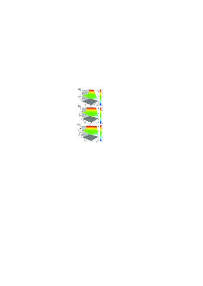
Figure 3: (color online) (a) Critical operation temperature $T_{el}^{OP}$ vs. $\Delta T$ and $V_{B}$ in the absence of the phonon’s thermal current; (b) $T_{el+ph}^{OP}$ vs. $\Delta T$ and $V_{B}$ in the presence of the phonon’s thermal current with $\lambda=10^{-17}$ Watt/K⁴; and (c) $T_{el+ph+heating}^{OP}$ vs. $\Delta T$ and $V_{B}$ in the presence of local heating and the phonon’s thermal current with $\lambda=10^{-17}$ Watt/K⁴.

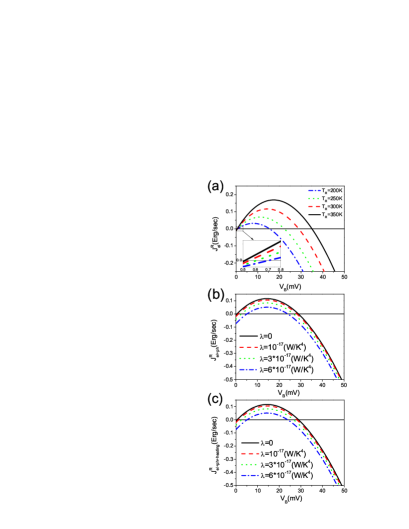
Figure 4: (color online) (a) $J_{el}^{R}$ vs. $V_{B}$ for various values of $T_{R}$ in the absence of the phonon’s thermal current, where $\Delta T=1~{}$K; (b) $J_{el+ph}^{R}$ vs. $V_{B}$ for $\lambda=0$, $1\times 10^{-17}$, $3\times 10^{-17}$, and $6\times 10^{-17}$ W/K⁴ in the presence of the phonon’s thermal current, where $\Delta T=1$ K and $T_{R}=300$ K; (c) $J_{el+ph+heating}^{R}$ vs. $V_{B}$ for $\lambda=0$, $1\times 10^{-17}$, $3\times 10^{-17}$, and $6\times 10^{-17}$ W/K⁴ in the presence of local heating and the phonon’s thermal current, where $\Delta T=1$ K and $T_{R}=300$ K.

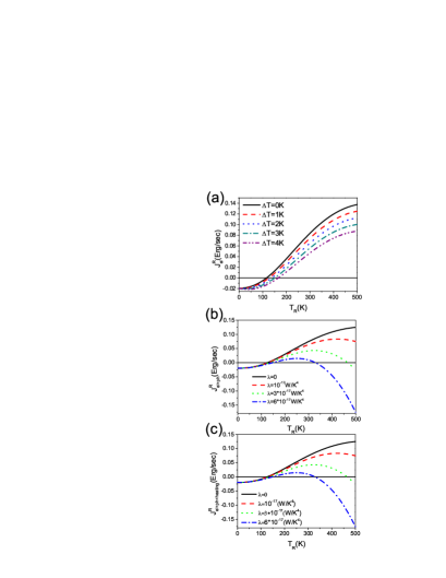
Figure 5: (color online) (a) $J_{el}^{R}$ vs. $T_{R}$ for various values of $\Delta T=0$, $1$, $2$, $3$, and $4$ K in the absence of the phonon’s thermal current, where $V_{B}=6$ mV; (b) $J_{el+ph}^{R}$ vs. $T_{R}$ for $\lambda=0$, $1\times 10^{-17}$, $3\times 10^{-17}$, and $6\times 10^{-17}$ W/K⁴ in the presence of the phonon’s thermal current, where $V_{B}=6$ mV; (c) $J_{el+ph+heating}^{R}$ vs. $T_{R}$ for $\lambda=0$, $1\times 10^{-17}$, $3\times 10^{-17}$, and $6\times 10^{-17}$ W/K⁴ in the presence of local heating and the phonon’s thermal current, where $V_{B}=6$ mV.

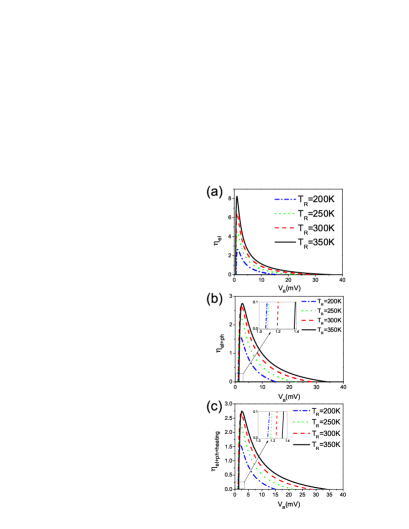
Figure 6: (color online) (a) COP ($\eta_{el}$) vs. $V_{B}$ in the absence of the phonon’s thermal current for $T_{R}=200$, $250$, $300$, and $350$ K, where $\Delta T=1$ K; (b) $\eta_{el+ph}$ vs. $V_{B}$ in the presence of the phonon’s thermal current for $T_{R}=200$, $250$, $300$, and $350$ K, where $\Delta T=1$ K; (c) $\eta_{el+ph+heating}$ vs. $V_{B}$ in the presence of local heating and the phonon’s thermal current for $T_{R}=200$, $250$, $300$, and $350$ K, where $\Delta T=1$ K.

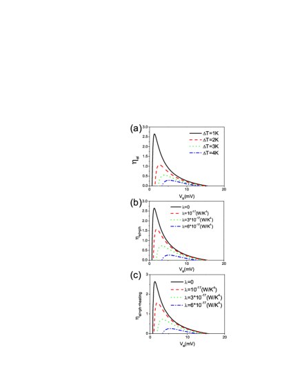
Figure 7: (color online) (a) $\eta_{el}$ vs. $V_{B}$ in the absence of the phonon’s thermal current for , where where $T_{R}=200$ K; (b) $\eta_{el+ph}$ vs. $V_{B}$ in the presence of the phonon’s thermal current for $\lambda=0$, $1\times 10^{-17}$, $3\times 10^{-17}$, and $6\times 10^{-17}$ W/K⁴, where where $\Delta T=1$ K and $T_{R}=200$ K; (c) $\eta_{el+ph+heating}$ vs. $V_{B}$ in the presence of local heating and the phonon’s thermal current for $\lambda=0$, $1\times 10^{-17}$, $3\times 10^{-17}$, and $6\times 10^{-17}$ W/K⁴, where where $\Delta T=1$ K and $T_{R}=200$ K.

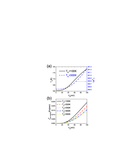
Figure 8: (color online) (a) Effective wire temperature $T_{w}$ vs. $V_{B}$ for $T_{R}=100$ K (left axis) and $T_{R}=300$ K (right axis), where $\lambda=1\times 10^{-17}$ W/K⁴; (b) The rate of heating energy dissipated to the cold reservoir $J_{local~{}heating}^{R}$ vs. $V_{B}$ for $T_{R}=100$, $200$, $250$, $300$, and $350$ K

This study proposes a thermoelectric cooling device based on an atomic-sized junction. We developed an analytical theory and first-principles calculations for the electronic cooling including the effect of the phonon’s thermal current and local heating. The theory is applied to investigate an ideal 4-Al monatomic chain sandwiched between two bulk Al electrodes. In the Sec. III. A., we discuss the enhanced Seebeck effect due to the $P_{x}-P_{y}$ orbital near the chemical potential and the influence of the phonon’s thermal current on $ZT$. A large Seebeck coefficient is of crucial importance for the design of thermoelectric nano-devices. Therefore, we investigate the thermoelectric properties of the 4-Al atomic junction as follows. In the Sec.  III. B, III. C, and III. D, we discuss the thermoelectric cooling effect without and with the phonon’s thermal current and local heating. The 4-Al thermoelectric junction serves as an example illustrating the advantage of nano-scale refrigerators, where the overwhelmingly Joule heat in the bulk system and photon radiation are strongly suppressed due to size reduction. These properties facilitate possible thermoelectric cooling in the 4-Al junction beyond the expectation of conventional solid-state device theory.

III.1 Thermoelectric Properties of the 4-Al Atomic Junction

We apply the theory and first-principles calculations shown in Sec. II to a 4-Al atomic junction as a thermoelectric cooling device, as depicted in Fig. 1(a). The 4-Al atomic junction is electronically simple such that the first-principle calculations reported here can be performed with a high level of accuracy. The aluminum junction is, therefore, an ideal testbed for comparing quantum transport theory under non-equilibrium and experiments Cuevas ; ThygesenAl .

We begin our discussion by considering an ideal 4-Al atomic chain bridging two bulk Al metal electrodes that we model as ideal metals (jellium model, $r_{s}\approx 2$). The nano-structured object is considered as a scattering center. The scattered wave functions of the whole system are calculated by solving the Lippmann-Schwinger equation iteratively until self-consistency is obtained. We assume that the left and right electrodes are independent electron and phonon reservoirs ($T_{R}=T_{C}$; $T_{L}=T_{R}+\Delta T=T_{H}$), respectively, with the electron and phonon population described by the Fermi-Dirac and Bose-Einstein distribution function. Two electrodes are connected to a battery with an applied bias $V_{B}=(\mu_{R}-\mu_{L})/e$, where $\mu_{L}$ and $\mu_{R}$ are the chemical potential deep in the left and right electrodes, respectively. A detailed account of the theory is given in Sec. II. A.

The Seebeck coefficients are calculated from first-principles using the transmission function obtained from the DFT calculations, as described in Eq. (9). The 4-Al atomic junction is marked by a sigma channel near the chemical potentials with the $P_{x}-P_{y}$ orbital characters, as shown in Fig. 1(b). The Seebeck coefficients correlate highly with the magnitudes and slopes of DOSs near the chemical potentials, as described in Eq. (11). The sigma channel leads to a large value in the slope of the transmission function near the chemical potentials. This give rise to a larger Seebeck coefficient, as shown in Fig. 1(c), which compares favorably with those of Pt, Pd, and Au atomic chains.

The efficiency of energy conversion in the thermoelectric junction is usually described by the figure of merit (denoted as $ZT$), as defined in Eq. (23). When $ZT$ tends to infinity, the thermoelectric efficiency will reach the Carnot efficiency, the upper limit of energy conversion efficiency. $ZT$ depends on the following physical factors: the Seebeck coefficient ($S$), the electric conductance ($\sigma$), the electron’s thermal conductance ($\kappa_{el}$), and the phonon’s thermal conductance ($\kappa_{ph}$). These physical factors can be evaluated using Eqs. (9), (18), (13), and (37), respectively. To obtain a large $ZT$ value, the thermoelectric nanojunction will require a large value of $S$, a large value of $\sigma$, and a small value of the combined heat conductance ($\kappa=\kappa_{el}+\kappa_{ph}$). Thermoelectric devices with a large value of $\sigma$ are usually accompanied by a large value of $\kappa_{el}$, due to the same proportionality with the transmission function. These values are highly correlated, making the enhancement of the thermoelectric figure of merit $ZT$ a challenging task.

The thermal energy carried by phonons flows from the hot into cold reservoir. The phonon’s thermal current takes heat into the cold reservoir and it ,thus, is a negative effect to the thermoelectric refrigeration. We consider the phonon’s thermal current in the weak link model [as described in Eq. (19)], where each electrode is assumed to be in thermodynamic equilibrium, joined by a weak mechanical link modeled by a harmonic spring of stiffness $K$. In the weak-tunneling limit, the weak link model can be interpreted as an application of the thermal Landauer formula Patton . Up to the leading order in temperatures, we expand Eq. (19) which gives a simple form, $J_{ph}^{R}=\lambda(T_{R}^{4}-T_{L}^{4})$ [i.e., Eq. (37) specified as the simplified weak link model], where $\lambda\approx 2\pi^{5}K^{2}C^{2}k_{B}^{4}/(15\hbar)$. Simplification allows us to investigate the effect of the phonon’s thermal current with a single parameter $\lambda$, which is determined by the stiffness of the nano-structured object ($K$) and the slope of the electrodes’s surface phonon’s spectral density ($C$). The simplified weak link model is valid in small temperature regime ($T\ll T_{D}$, where $T_{D}=394$ K is the Debye temperature for Al). We note that the simplified weak link model violates the Wiedemann-Franz law in low-temperature regime, while Eq. (19) restores the Wiedemann-Franz law at $T\gg T_{D}$. The range of temperatures discussed in this study mostly lies within the valid regime of the simplified weak link model. Therefore, we consider $ZT$ as a function of temperatures in the presence of the phonon’s thermal current of which is represented by various values of $\lambda$, as shown in Fig. 1(d). The validity of the $\lambda$ values for linear atomic wires will be justified later in Sec. III. C.

III.2 Thermoelectric Cooling Effect in the Absence of Phonon’s Thermal Current and Local Heating

Let us now attempt to investigate the 4-Al junction as a thermoelectric cooling device from the first-principles approaches. For the present, we shall confine our attention to the simplest case, the one which neglects the phonon’s thermal current and local heating. Effects of the phonon’s thermal current and local heating will be discussed in the Sec. III. C and III. D. We also put forward an analytical theory to explain the numerical results. The analytical theory described below is general to any atomic/molecular thermoelectric junction as a thermoelectric nano-refrigerator.

When an external bias is applied, electrons flow from the right to the left electrodes. The flow of electrons carries not only the charge current but also the energy current. The thermal current carried by electrons [denoted as $J_{el}^{R(L)}(\mu_{L},T_{L};\mu_{R},T_{R})$], defined as the rate at which thermal energy flows from the right (into the left) electrode, can be calculated from first-principles using Eq. (7) with the help of the wavefunctions obtained self-consistently in the DFT calculations. Note that $J_{el}^{R}+IV_{B}=J_{el}^{L}$ [for details see Eq. (24)] because of energy conservation. It implies that the thermoelectric refrigeration requires electric power $IV_{B}$ to remove thermal energy from the cold (right) reservoir (with rate $J_{el}^{R}$) and reject waste thermal energy to the hot (left) reservoir (with rate $J_{el}^{R}$). The nano-refrigerator works when $J_{el}^{R}>0$. As noted in Eq. (7), $J_{el}^{R}$ is a function of $V_{B}$, $\Delta T$, and $T_{R}$. Note that $J_{el}^{R}(T_{R}=0)<0$. At a given $V_{B}$ and $\Delta T$, the smallest solution of $J_{el}^{R}(T_{R})=0$ defines the threshold operation temperature, denoted as $T_{el}^{OP}$, below which the nano-refrigerator does not function. Figure 3(a) shows the $T_{el}^{OP}$ of the 4-Al nano-refrigerator as a function of $\Delta T$ and $V_{B}$. The operating temperature of the 4-Al nano-refrigerator can be lower than $100$ K, as shown in Fig. 3(a).

To enrich the understanding of thermoelectric nano-refrigerators, we also propose an analytical theory that provide guidelines for the design of nano-refrigerators. When $\Delta T\ll T_{R}$, the application of the Sommerfeld expansion on Eq. (7) can simplify the electron’s thermal current $J_{el}^{R}$ as a polynomial of $V_{B}$, as described in Eq. (27). If the higher-order term $V_{B}^{3}$ is neglected, the maximum of $J_{el}^{R}(T_{R})$ that is greater than zero yields a criterion for the existence of thermoelectric cooling, which gives Eq. (28): $-S>\pi k_{B}\sqrt{2\Delta T/(3T_{C})}/e$, where $T_{C}$ ($=T_{R}$) is the temperature of the cold (right) reservoir, $S=-\pi^{2}k_{B}^{2}\tau^{\prime}(\mu)T_{R}/[3e\tau(\mu)]$ is the Seebeck coefficient, $k_{B}$ is the Boltzmann constant, and $e$ is the electron charge. To have possible refrigeration effect, the Seebeck coefficient $S$, the temperature difference $\Delta T$, and the temperature of the cold reservoir $T_{C}$ need to satisfy Eq. (28). The choice of an n-type thermoelectric junction with a large Seebeck coefficient is of crucial importance in the design of thermoelectric nano-refrigerators. Large Seebeck coefficients could be achieved through an appropriate choice of bridging nano-structured objects and further optimized by applying gate voltages Wang ; Liu .

Figure 4(a) shows the rate of thermal energy extracted from the cold temperature reservoir ($J_{el}^{R})$ as a function of $V_{B}$ for $T_{R}=200$, $250$, $300$, and $350$ K, where the temperature difference between the hot and cold reservoir $\Delta T$ is fixed at $1$ K. We note that $J_{el}^{R}<0$ at zero bias [see Fig. 4(a)], and thus a lower threshold voltage $V_{el}^{th,lower}$ for the battery is needed to trigger the refrigeration effect. The lower threshold bias is defined as the smallest positive solution of $J_{el}^{R}(V_{B})=0$ for a given $T_{R}$ and $\Delta T$. When $V_{B}<V_{el}^{th,lower}$, the rate of thermal energy removed from the cold reservoir is negative ($J_{el}^{R}<0$) and thus the thermoelectric nano-refrigerator does not function. We also observe an upper threshold voltage $V_{el}^{th,upper}$ for the refrigeration effect. When $V_{B}>V_{el}^{th,upper}$, the rate of thermal energy removed from the cold reservoir is also negative ($J_{el}^{R}<0$) and thus the thermoelectric nano-refrigerator loses the capability of refrigeration. Since $V_{el}^{th,lower}$ and $V_{el}^{th,upper}$ have very small values, we neglect the terms higher than the second order of $V_{B}$ in Eq. (27) and obtain $V_{el}^{th,lower}$ and $V_{el}^{th,upper}$ from $J_{el}^{R}(V_{B})=0$, as described in Eqs. (29) and (30), where we assumed $\Delta T\ll T_{R}$. Equation (29) predicts that the lower threshold voltage, $V_{el}^{th,lower}\approx-\pi^{2}k_{B}^{2}\Delta T/(3e^{2}ST_{R})$, decreases as $T_{R}$ increases, as shown in the inset of Fig. 4(a). Equation (30) predicts that the upper threshold voltage, $V_{th,upper}^{el}\approx 2ST_{R}^{2}$, increases as $T_{R}$ increases. Concluding from Eqs. (29), (30) and (35), the refrigeration effect is triggered at around $V_{B}=V_{el}^{th,lower}$, optimized around $V_{B}=2V_{el}^{th,lower}$, and loses the refrigeration capability at $V_{B}=V_{el}^{th,upper}$.

Figure 5(a) shows $J_{el}^{R}$ as a function of $T_{R}$ for different values of $\Delta T=0$, $1$, $2$, $3$, and $4$ K, where the bias is fixed at $V_{B}=6$ mV. For a given $V_{B}$ and $\Delta T$, we define the critical operation temperature $T_{el}^{OP}$ as the solution of $J_{el}^{R}(T_{R})=0$. The thermoelectric nano-refrigerator is working when $T_{R}>T_{el}^{OP}$. The critical operation temperature can be calculated from Eq. (26): $T_{el}^{OP}\approx\frac{1}{2}[(\alpha-1)\Delta T+\sqrt{(\alpha^{2}-1)\Delta T^{2}+\beta}]$, where $\alpha=\tau(\mu_{L})/[\tau^{\prime}(\mu_{L})eV_{B}]$ and $\beta=-2V_{B}/S$. The foregoing equation predicts that $T_{el}^{OP}$ increases as $\Delta T$ increases, which agrees well with the numerical calculation presented in Fig. 5(a). If $\Delta T=0$ K, then $T_{el}^{OP}$ reaches the minimum value $\left(T_{el}^{OP}\right)_{\min}\approx\sqrt{T_{R}V_{B}/(-2S)}$ as described in Eq. (32). The equation shows that $\left(T_{el}^{OP}\right)_{\min}$ increases as $V_{B}$ increases and as $T_{R}$ increases, respectively. At $V_{B}=6$ mV, the $\left(T_{el}^{OP}\right)_{\min}$ for the 4-Al thermoelectric refrigerator is $116$ K, which can be further suppressed by decreasing the bias $V_{B}$ . Turning to the efficiency of the thermoelectric nano-refrigerator, the COP (denoted as $\eta^{el}$) is defined as the ratio of the rate of heat removed from the cold reservoir to the electric power supplied by the battery, that is, $\eta_{el}=J_{el}^{R}/(IV_{B})$, as equivalent to Eq. (33). Derived from Eq. (34), the maximum value of COP is given by Eq. (35).

Figure 6(a) shows the numeric calculations of $\eta_{el}$ as a function of $V_{B}$ for $T_{R}=200$, $250$, $300$, and $350$ K, where $\Delta T=1$ K. This figure also shows that the optimized COP ($\eta_{el}^{\max}$) increases as $T_{R}$ increases. The optimized COP occurs at bias $V_{\max}^{\eta_{el}}\approx 2V_{el}^{th,lower}$, where $V_{el}^{th,lower}$ is the lower threshold bias for possible refrigeration, as shown in Fig. 7(a). We should note that the maximum value of COP can be greatly magnified by a suitable nanojunction with a large Seebeck coefficient according to $\eta_{el}^{\max}\propto S^{2}$ as predicted in Eq. (35).

Figure 7(a) shows the numeric calculations of $\eta_{el}$ as a function of $V_{B}$ for $\Delta T=1$, $2$, $3$, and $4$ K, where $T_{R}=200$ K. The exchange of energy by heat currents between the hot and cold reservoirs is an irreversible process, and leads the decrease of the optimized COP as $\Delta T$ increases as described by Eq. (35): $\eta_{el}^{\max}=3e^{2}S^{2}T_{R}/(4\pi^{2}k_{B}^{2}\Delta T)-1/2$. As a direct consequence of the above equation, the maximum value of COP ($\eta_{el}^{\max}$) increases as $T_{R}$ increases and as $\Delta T$ decreases. This prediction agrees well with Eq. (35).

III.3 Thermoelectric Cooling Effect including the Phonon’s Thermal Current

The phonon’s thermal current carries thermal energy from the hot to cold reservoir, which is an adverse effect to refrigeration. To assess the extent of this adverse effect, we consider the phonon’s thermal current within the simplified weak link model. The simplified weak link model is suitable for describing the heat transport for two thermal reservoirs connected by a weak elastic link in a low temperature regime ($T\ll T_{D}$, where $T_{D}=394$ K is the Debye temperature for Al) and is convenient to describe the phonon’s thermal current by a single parameter $\lambda$: $J_{ph}^{R}=\lambda(T_{R}^{4}-T_{L}^{4})$, where $\lambda\approx 2\pi^{5}K^{2}C^{2}k_{B}^{4}/(15\hbar)$. The parameter $\lambda$ can be determined by $K$ and $C$, where $K$ is the stiffness of the nano-structured object connecting to electrodes and $C$ is the slope of the spectral density $N(E)\approx C\times E$. The simplified weak link model allows the construction of an analytical theory that offers a concise explanation for how the phonon’s thermal current (represented by a single parameter $\lambda$) affects thermoelectric cooling.

From recent experiments Shiota , it is observed that the stiffness of the linear Pt atomic chains varies in a wide range of several orders of magnitudes. This experiment suggests that the stiffness ($K\approx 0$ to $1.2$ N/m) is likely to depend strongly on the detailed atomic structure of the full system, especially in the contact region. For example, the monatomic chain could be particularly stiff along the chain direction when the atomic chain forms a perfectly straight line; otherwise, the atomic (zigzag) chain could easily bend with much smaller stiffness. In this view, the magnitudes of phonon’s thermal current could possibly vary in a wide range in nanojunctions formed by monatomic chains. This feature could allow the possibility (for example, zigzag chain instead of perfect linear chain) to suppress the phonon’s thermal current by creating a suppression in the mechanic link. An estimation from the experimental data of $K=0$ to $1.2$ N/m and $C\approx 1.887\times 10^{8}$ cm²/erg² in the Pt atomic junction yields the values of $\lambda$ range to be from $0$ to $2.05\times 10^{-19}$ W/K⁴  Shiota ; Kern .

In the 4-Al atomic junction, we choose $\lambda$ around the order of $10^{-17}$ W/K⁴ to present the strength of the phonon’s thermal current. In this range of $\lambda$, the effect of the phonon’s thermal current on the thermoelectric refrigeration is salient. For the 4-Al monatomic junction, $\lambda\approx 5.7\times 10^{-15}$ Watt/K⁴, which is given by $K\approx 90.91$ N/m obtained from total energy calculations and $C\approx 7.62\times 10^{8}$ cm²/erg² from the surface phonon dispersion relation obtained from first-principle calculations Chulkov . However, this value is notably larger than the Pt monatomic chains with $\lambda$ ranging from $0$ to $2.05\times 10^{-19}$ W/K⁴. The reason for this is that the stiffness of a 4-Al linear atomic chain is $K=90.91$ N/m, which is notably larger than the stiffness of Pt chain ($K=0$ to $1.2$ N/m) measured in the experiments. This experiment for Pt monatomic chain infers that the stiffness $K$ for the 4-Al junction could be overestimated by the total energy calculations, where the chain is assume to be perfectly linear. In this viewpoint, the $\lambda$ (around $10^{-17}$ W/K⁴) we choose to present the strength of the phonon’s thermal current for the 4-Al atomic junction could be reasonable.

In the presence of the phonon’s thermal current, the COP is defined as $\eta_{el+ph}=\frac{J_{el+ph}^{R}}{IV_{B}}$, where $J_{el+ph}^{R}=J_{el}^{R}+J_{ph}^{R}$ is the combined thermal current. In the presence of the phonon’s thermal current, the functioning of the 4-Al atomic refrigerator requires higher operation temperatures (denoted as $T_{el+ph}^{OP}$), as shown in Fig. 3(b), where we plot the operation temperature $T_{el+ph}^{OP}$ as a function of $V_{B}$ and $\Delta T$ with the strength of the phonon’s thermal current described by the simplified weak link model with $\lambda=10^{-17}$ W/K⁴. Applying the Sommerfeld expansion, the combined thermal current $J_{el+ph}^{R}$ can be expressed as a polynomial of $V_{B}$ when $\Delta T\ll T_{R}$, as shown in Eq. (40). When the term $V_{B}^{3}$ is neglected in Eq. (40), the criterion for the existence of electronic cooling is given by Eq. (41): $-S>\sqrt{\left(2\pi^{2}k_{B}^{2}/(3e^{2})+8\lambda/\sigma\right)\left(\Delta T/T_{R}\right)}$. The criterion for possible thermoelectric refrigeration provides the guideline for devising experiments to test the effect of thermoelectric cooling at the atomic level. When $\lambda\rightarrow 0$, Eq. (41) restores Eq. (28) in the absence of the phonon’s thermal current.

Figure 4(b) shows the combined thermal current $J_{el+ph}^{R}$ as a function of $V_{B}$ for $\lambda=0$, $1\times 10^{-17}$, $3\times 10^{-17}$, and $6\times 10^{-17}$ W/K⁴, where we fix $\Delta T=1$ K and $T_{R}=300$ K. Note that $J_{el+ph}^{R}<0$ at zero bias. Similar to the previous discussions in the absence of the phonon’s thermal current, the thermoelectric nano-refrigerator works when $J_{el+ph}^{R}>0$. This leads to the lower and upper bounds of threshold voltage, as given in Eqs. (42)] and (43). The working bias which allows the operation of the thermoelectric nano-refrigerator is restricted to a small range of bias: $V_{el+ph}^{th,lower}<V_{B}<V_{el+ph}^{th,upper}$. Eqs. (43) and (43) show that the lower (upper) threshold bias $V_{el+ph}^{th,lower}$ ($V_{el+ph}^{th,upper}$) increases (decreases) by a value of $\lambda\left[4T_{R}^{2}\Delta T/\left(-S\right)\sigma\right]$ as the intensity of the phonon’s thermal current ($\lambda$) increases. This leads to suppression of the range of working biases by the phonon’s thermal current, which agrees well with the numerical calculations as shown in Fig. 4(b).

Figure 5(b) shows the combined thermal current $J_{el+ph}^{R}$ as a function of $T_{R}$ for $\lambda=0$, $1\times 10^{-17}$, $3\times 10^{-17}$, and $6\times 10^{-17}$ W/K⁴, where we fix $V_{B}=6$ mV and $\Delta T=1$ K. Figure 5(b) exhibits the combined thermal current $J_{el+ph}^{R}$, which could become negative at high temperatures regime. The reason for this is that the phonon’s thermal current brings heat from the hot to the cold reservoir. Thus, the combined thermal current becomes a negative value, which disables refrigeration capability at high temperatures. This imposes an upper limit for the working temperature, above which $J_{el+ph}^{R}$ turns to be negative and consequently the nano-refrigerator does not function. The operation of nano-refrigerator is limited to a range of temperatures between $T_{low,el+ph}^{OP}$ and $T_{high,el+ph}^{OP}$, as described in Eqs. (44) and (45). As $\lambda$ increases, Eqs. (44) and (45) predict that the range of operation temperatures shrinks, which agrees well with the numerical calculations as shown in Fig. 5(b).

Figure 6(b) shows the numeric calculations of $\eta_{el+ph}$ as a function of $V_{B}$ for $T_{R}=200$, $250$, $300$, and $350$ K, where $\Delta T=1$ K is fixed. Equation (46) shows the upper limit of COP (denoted as $\eta_{el+ph}^{\max}$) is given by : $\eta_{el+ph}^{\max}=\left[\left(\eta_{el}^{\max}\right)^{-1}+\lambda\left(16T_{R}\Delta T/(S^{2}\sigma)\right)\right]^{-1}$.  It shows that the upper limit of COP ($\eta_{\max}^{el+ph}$) increases as $\lambda$ increases as predicted by Eq. (46); meanwhile, the inset of Fig. 6(b) shows that the $V_{el+ph}^{th,lower}$ increases as $T_{R}$ increases, as predicted by Eq. (42) valid for $\Delta T\ll T_{R}$. Equation (46) also predicts that and $\eta_{\max}^{el+ph}$ increases as $S^{2}\sigma$ decreases, indicating that a large value of Seebeck coefficient is of critical importance for efficient thermoelectric refrigeration.

Figure 7(b) shows the numeric calculations of $\eta_{el+ph}$ as a function of $V_{B}$ for $\lambda=0$, $1\times 10^{-17}$, $3\times 10^{-17}$, and $6\times 10^{-17}$ W/K⁴, where $\Delta T=1$ K and $T_{R}=200$ K.It shows that the upper limit of COP ($\eta_{el+ph}^{\max}$ ) decreases as the strength of phonon’s thermal current increases because the phonon’s thermal current is an adverse effect to refrigeration. Figure 7(b) also shows that the lower threshold bias $V_{el+ph}^{th,lower}$ increases as $\lambda$ increases and agrees well with the prediction of Eq. (42).

In short, the phonon’s thermal current, which is relevant to the mechanical coupling between the nano-structured object and the electrodes, is an adverse effect to refrigeration. To minimize the adverse effect, we suggest creating a weak mechanical link between the nano-structured object and the electrodes while still allowing electrons to tunnel.

III.4 Thermoelectric Cooling Effect Including the Phonon’s Thermal Current and Local Heating

We further consider the effect of local heating on the thermoelectric refrigeration. Electrons that travel with energies larger than the energy of normal modes can excite corresponding vibrations in the nano-structure anchoring the electrodes. This effect causes local heating in the nano-structure chenheating ; Frederiksen ; Huang2 . Local heating occurs when electrons exchange energy with the excitation and relaxation of the energy levels of the vibration of the nano-structured object that anchors the electrodes. The nano-object bridging the junction is formed by few atoms, and thus the dispersion relation of phonon is characterized by the lack of Goldstone mode. When normal coordinates are considered, the complex vibrations of nano-object connecting to heavy electrodes can be cast into a set of independent simple harmonic oscillators described as normal modes. Due to the selection rule, the contributions to local heating from modes with large vibrational components along the direction of propagating electrons are important chenh2 . The smallest longitudinal normal mode has an energy of $eV_{onset}\approx 20$ meV Yang .

The heat generated in the central wire region can be dissipated to the bulk electrodes via phonon-phonon interactions. The heat generation eventually equilibrates the heat dissipation, where the wire region reaches an effective local temperature $T_{w}$ higher than the averaged electrode temperatures $(T_{L}+T_{R})/2$. Local temperature depends on several factors: the strength of coupling between electrons and the vibrations, the background temperature, and the mechanical coupling between the nano-structure and electrodes which determines the efficiency of thermal current dissipating the thermal energy of local heating.

In Fig. 8(a) we show the effective wire temperature ($T_{w}$) as a function of bias ($V_{B}$) for $T_{R}=100$ and $300$ K, where we assume that the strength of the phonon’s thermal current is given by $\lambda=1\times 10^{-17}~{}$W/K⁴. For $T_{R}=100$ K, the increase of local wire temperature $T_{w}$ is noticeable when $V_{B}>V_{onset}\approx 20$ mV. We note that $T_{w}$ is slightly higher than $T_{R}$ when $V_{B}<V_{onset}$ because only a small portion of electrons has energy larger than $eV_{onset}$ due to the tail of the Fermi-Dirac distributions at finite temperatures. For $T_{R}=300$ K, the increase in local wire temperature $T_{w}$ is significantly suppressed due to increasingly efficient heat dissipation at high temperatures. The local heating generated in the wire region is dissipated to the left (hot) and right (cold) electrodes as described in Eqs. (54) and (55), respectively. The combined thermal current including the effect of the phonon’s thermal current and local heating ($J_{el+ph+heating}^{R}$) is given by Eq. (57).

In Fig. 8(b)we show the rate of local heating energy which is dissipated to the cold (right) electrode ($J_{local~{}heating}^{R}$) as a function of bias ($V_{B}$) for $T_{R}=100$, $200$, $250$, $300$, and $350$ K, where we assume that the strength of the phonon’s thermal current is given by $\lambda=1\times 10^{-17}$ W/K⁴. The rate of heating energy dissipated to the right (cold) electrode ($J_{local~{}heating}^{R}$) introduces an additional negative effect to refrigeration, and, thus, the combined thermal current $J_{el+ph+heating}^{R}$ which takes heat energy from the right (cold) reservoir to left (hot) reservoir is suppressed. In this bias range, the heating power is smaller than 1% of the electric power ($IV_{B}$) supplied by a battery even at ambient temperatures because of the quasi-ballistic transport. This fact leads to $J_{local\text{ }heating}^{R}\ll J_{ph}^{R}$ in the range of working biases ($V_{el+ph}^{th,lower}<V_{B}<V_{el+ph}^{th,upper}$) for the $\lambda$ values we considered in this study. Consequently, the effect of local heating on thermoelectric refrigeration is negligible when the phonon’s thermal current is included. This finding has profound implications on the design of nanoscale thermoelectric refrigerator, where the local heating is strongly suppressed such that the overwhelming Joule heating in the bulk system can be avoided. This feature remarkably facilitates the electron cooling beyond the expectation of the conventional thermoelectric device theory.

We repeat the calculations in the previous two subsections. The results are not visibly different when we compare the ones that include contributions from both phonon’s thermal current and local heating, as shown in Figs. 4(c), 5(c), 6(c), and 7(c), with the ones that has phonon’s thermal current only, as shown in Figs. 4(b), 5(b), 6(b), and 7(b).

IV Conclusions

In summary, we propose a thermoelectric nano-refrigerator based on an atomic junction, the extreme limit of device minimization. In-depth research which combines the first-principles and analytical calculations is developed to study the thermoelectric cooling mechanism. The theory is applied to investigate the thermoelectric cooling of the 4-Al monatomic junction. The 4-Al junction is electronically simple such that the first-principle calculations reported here can be performed with a high level of accuracy. It, thus, serves an ideal testbed for comparing the prediction of the theory and experiments. Our studies show that the $P_{x}-P_{y}$ orbital characters near the chemical potential lead to a larger Seebeck coefficient in the 4-Al atomic junction. We investigated the working conditions, operation temperatures, electron’s thermal current which removes heat from the cold temperature reservoir, and COP in the presence of the phonon’s thermal current and local heating.

Firstly, we perform first-principles calculations for the electron’s thermal current ($J_{el}^{R}$) which removes heat from the cold temperature reservoir in the absence of the phonon’s thermal current and local heating. The thermoelectric cooling is working when $J_{el}^{R}>0$. It is observed that the operation of nano-refrigerators requires a minimum critical working temperature. The solution of $J_{el}^{R}(T_{R})=0$ defines the critical operation temperature denoted as $T_{el}^{OP}$. When $T_{R}<T_{el}^{OP}$, nano-refrigerators do not function. When $\Delta T=0$, $T_{el}^{OP}$ reaches the minimum value $(T_{el}^{OP})_{\min}$, as given by Eq. (32). It is observed that the lowest critical operation temperature may be smaller than $100$ K, which is very efficient as a low-temperature operated nano-refrigerator compared with the vacuum diode due to reduced work function via resonant tunneling. The working condition of the thermoelectric nano-refrigerator is quite demanding. The applied voltage is restricted to a small range of biases. It is observed that there are lower and an upper bounds of biases denoted as $V_{th}^{el}$ and $V_{upperth}^{el}$, respectively. The thermoelectric nano-refrigerator does not work when the applied biases are smaller than $V_{th}^{el}$ or larger than $V_{upperth}^{el}$. Since the lower and upper threshold biases are small, it allows us to expand $J_{el}^{R}$ and obtain an analytical expression for $V_{th}^{el}$ and $V_{upperth}^{el}$, as described in Eqs. (29) and (30). The maximum value of COP ($\eta^{el}$) occurs at bias around $2V_{th}^{el}$ and can be analytically expressed as Eq. (35).

Secondly, we consider the phonon’s thermal current, which is a major effect against the operation of atomic refrigerators. To have a more perspective realization, we consider the phonon’s thermal current in the approximation of the simplified weak-link model: $J_{ph}^{R}=\lambda(T_{R}^{4}-T_{L}^{4})$. The simple model has a single parameter ($\lambda$) which allows us to construct an analytical theory to show the effect of the phonon’s thermal current on electronic cooling in a transparent way. We choose $\lambda$ around the order of $10^{-17}$ W/K⁴ to present the effect of the phonon’s thermal current. In this range of $\lambda$, the effect of the phonon’s thermal current on the thermoelectric refrigeration is salient and sensitive. In the presence of the phonon’s thermal current, the combined thermal current ($J_{el+ph}^{R}$) which removes heat from the cold temperature reservoir decreases as $\lambda$ increases. This leads to higher critical operation temperature $T_{el+ph}^{OP}$. The working conditions of the thermoelectric nano-refrigerator are hampered by the phonon’s thermal current further, as described in Eq. (41). The range of biases which are allowed to drive nano-refrigerators shrinks. The lower bound of the operating bias ($V_{th}^{el+ph}$) increases as the intensity of the phonon’s thermal current ($\lambda$) increases, as described in Eq. (42). The upper bound of the operating bias ($V_{upperth}^{el+ph}$) decreases as $\lambda$ increases. The COP ($\eta^{el+ph}$) is also suppressed by the intensity of the phonon’s thermal current ($\lambda$) because the phonon’s thermal current, taking heat from the hot to cold temperature reservoir, is an adverse effect to thermoelectric refrigeration. The suppression of the optimized COP ($\eta_{\max}^{el+ph}$) by $\lambda$ agrees well with the analytical expression given by Eq. (46). We would like to stress that the $\lambda$ values chosen to present the strength of the phonon’s thermal current is quite large. For example, the rate of thermal energy flows from electrode at $100$ K to electrode at $0$ K is $1$ nW when $\lambda=1\times 10^{-17}$ W/K⁴.

Thirdly, we consider the effect of local heating on the thermoelectric refrigeration. Electrons that propagate with the energies larger than the energies of normal modes can excite corresponding vibrations in the nano-object anchoring the electrodes. This effect causes local heating in the nano-structure, which is analogous to Joule heating in the bulk system caused by diffusive electrons. The heat generated in the center region of the junction is dissipated to the hot and cold temperature reservoirs; and, thus, local heating is an adverse effect to electronic cooling. In the bulk system, irreversible Joule heating is overwhelming such that the efficiency of a thermoelectric refrigerator is significantly suppressed. Fortunately, the quasi-ballistic nature of electron transport in the atomic scale junctions significantly reduces local heating due the size reduction. This quantum feature remarkably facilitate thermoelectric cooling beyond the expectation of the conventional thermoelectric device theory. To demonstrate this point, we perform first-principles calculations for local heating using the Fermi golden rule in the first-order perturbation theory in the frame work of density functional theory. Our calculations show that local heating dissipated to the cold temperature reservoir is very small compared with the large phonon’s thermal current considered in this study. Consequently, local heating is negligible, especially in the small bias regime where the nano-refrigerants is functioning. Moreover, the photon radiation is also negligible even when we consider the perfect black body radiation for a nanojunction with a surface area of $1$ $\mu$m diameter compared with the large phonon’s thermal current.

Finally, we would like to mention that the simplified weak link model may not be perfect in quantitative description of the phonon’s thermal current. For example, it is valid only when for $T\ll T_{D}$, where $T_{D}=394$ K is the Debye temperature for Al. The value of $\lambda\approx 2\pi^{5}K^{2}C^{2}k_{B}^{4}/(15\hbar)$ is unknown due to the uncertainty of the stiffness $K$ of the bridging nano-object. For the 4-Al monatomic junction, $\lambda\approx 5.7\times 10^{-15}$ Watt/K⁴where $K\approx 90.91$ N/m is obtained from total energy calculations and $C\approx 7.62\times 10^{8}$ cm²/erg² is obtained from the surface phonon dispersion relation from electronic-structure calculations. This $\lambda$ value is considerably larger than the Pt monatomic chains with $\lambda$ ranging from $0$ to $2.05\times 10^{-19}$ W/K⁴, where $K=0\char 126\relax 1.2$ N/m is obtained from the experiments and $C=1.887\times 10^{8}$ cm²/erg² is obtained from the surface phonon dispersion relation of Pt. The reason for large discrepancy between the $\lambda$ value is as the following: the stiffness of a 4-Al linear atomic chain ($K=90.91$ N/m) from total energy calculations is much larger than the stiffness of Pt monatomic chain ($K=0\char 126\relax 1.2$ N/m) measured in experiments. This comparison infers that the stiffness $K$ is likely to depend strongly on the detailed atomic structure of the full system, especially in the contact region. For example, the atom chain could be particularly stiff along the chain direction when the atomic chain forms a perfectly straight line; otherwise, the atomic (zigzag) chain could easily bend with much smaller stiffness. The total energy calculations have assumed that the atomic chain is perfectly linear. This may lead to significant overestimation for the $\lambda$ value. The imperfection of the contact region in the real system may allow the possibility (for example, zigzag chain instead of perfect linear chain) to suppress the phonon’s thermal current by creating a frustration in the mechanical link connecting to the electrodes. In this case, the thermoelectric refrigeration at atomic scale may be salient.

In short, atomic-level control of the contact region is expected to open new opportunities and challenges in developing new forms of thermoelectric energy conversion devices. Atomic scale thermoelectric devices need to be extended by the utilization of unprecedented experiments. The nano-refrigerators potentially have better performance than the conventional TE refrigerators with the same $ZT$. The is due to the suppression of local heating and photon radiation due to the small size, which avoid the overwhelming Joule heating in the bulk system. This feature remarkably facilitates the electron cooling beyond the expectation of the conventional thermoelectric device theory.

The authors thank MOE ATU, NCHC, National Center for Theoretical Sciences(South), and NSC (Taiwan) for support under Grants NSC 97-2112-M-009-011-MY3, 098-2811-M-009-021, and 97-2120-M-009-005.

References

- (1) A. Aviram and M. A. Ratner, Chem. Phys. Lett. 29, 277 (1974).
- (2) M. Di Ventra, Electrical transport in nanoscale systems, (Cambridge University Press, Cambridge, 2008).
- (3) C. C. Kaun and H. Guo, Nano Lett. 3, 1521 (2003).
- (4) M. Di Ventra and N. D. Lang, Phys. Rev. B 65, 045402 (2001).
- (5) A. Nitzan and M. A. Ratner, Science 300, 1384 (2003).
- (6) M. Kamenetska, S. Y. Quek, A. C. Whalley, M. L. Steigerwald, H. J. Choi, S. G. Louie, C. Nuckolls, M. S. Hybertsen, J. B. Neaton, and L. Venkataraman, J. Am. Chem. Soc. 132, 6817 (2010).
- (7) G. C. Solomon, C. Herrmann, T. Hansen, V. Mujica, and M. A. Ratner, Nature Chemistry 2, 223 (2010).
- (8) W. Wang, T. Lee, I. Kretzschmar, and M. A. Read, Nano Lett. 4, 643 (2004).
- (9) M. Galperin, A. Nitzan, and M. A. Ratner, Phys. Rev. B 78, 125320 (2008).
- (10) J. Jiang, M. Kula, W. Lu, and Y. Luo, Nano Lett. 5, 1551 (2005).
- (11) L. H. Yu, C. D. Zangmeister, J. G. Kushmerick, Phys. Rev. Lett. 98, 206803 (2007).
- (12) M. Paulsson, T. Frederiksen, and M. Brandbyge, Nano Lett. 6, 258 (2006).
- (13) G. C. Slomon, A. Gagliardi, A. Pecchia, T. Frauenheim, A. Di Carlo, J. R. Reimers, and N. S. Noel, J. Chem. Phys. 124, 094704 (2006).
- (14) Y. C. Chen, M. Zwolak, and M. Di Ventra, Nano Lett. 5, 621 (2005).
- (15) Y. C. Chen, Phys. Rev. B 78, 233310 (2008).
- (16) I. S. Kristensen, M. Paulsson, K. S. Thygesen, and K. W. Jacobsen, Phys. Rev. B 79, 235411 (2009).
- (17) D. Djukic and J. M. van Ruitenbeek, Nano Lett. 6, 789 (2006).
- (18) M. Kiguchi, O. Tal, S. Wohlthat, F. Pauly, M. Krieger, D. Djukic, J. C. Cuevas, and J. M. van Ruitenbeek, Phys. Rev. Lett. 101, 046801 (2008).
- (19) P. J. Wheeler, J. N. Russom, K. Evans, N. S. King, and D. Natelson, Nano Lett. 10, 1287 (2010).
- (20) Y. C. Chen and M. Di Ventra, Phys. Rev. Lett. 95, 166802 (2005).
- (21) Y. S. Liu and Y. C. Chen, cond-mat/arXiv:1005.3407.
- (22) Y. C. Chen, M. Zwolak, and M. Di Ventra, Nano Lett. 3, 1691 (2003).
- (23) Z. Huang, B. Xu, Y. C. Chen, M. Di Ventra, and N. J. Tao, Nano Lett. 6, 1240 (2006).
- (24) M. Di Ventra, S. T. Pantelides, and N. D. Lang, Appl. Phys. Lett. 76, 3448 (2000).
- (25) C. L. Ma, D. Nghiem, and Y. C. Chen, Appl. Phys. Lett. 93, 222111 (2008).
- (26) P. M. Solomon and N. D. Lang, ACS Nano 2, 435 (2008).
- (27) N. D. Lang and P. M. Solomon, ACS Nano 3, 1437 (2009).
- (28) H. Song, Y. Kim, Y. H. Jang, H. Jeong, M. A. Reed, and T. Lee, Nature 462, 1039 (2009).
- (29) C. H. Ahn, A. Bhattacharya, M. Di Ventra, J. N. Eckstein, C. D. Frisbie, M. E. Gershenson, A. M. Goldman, I. H. Inoue, J. Mannhart, A. J. Millis, A. F. Morpurgo, D. Natelson, and J. M. Triscone, Rev. Mod. Phys. 78, 1185 (2006).
- (30) S. M. Lindsay and M. A. Ratner, Advanced Materials 19, 23 (2007).
- (31) N. J. Tao, Nat. Nanotechnol. 1, 173 (2006).
- (32) B. Ludoph and J. M. van Ruitenbeek, Phys. Rev. B 59, 12290 (1999).
- (33) P. Reddy, S. Y. Jang, R. A. Segalman, and A. Majumdar, Science 315, 1568 (2007).
- (34) K. Baheti, J. A. Malen, P. Doak, P. Reddy, S. Y. Jang, T. D. Tilley, A. Majumdar, and R. A. Segalman, Nano Lett. 8, 715 (2008).
- (35) J. A. Malen, P. Doak, K. Baheti, T. D. Tilley, R. A. Segalman, and A. Majumdar, Nano Lett. 9, 1164 (2009).
- (36) J. A. Malen, S. K. Yee, A. Majumdar, and R. A. Swgalman, Chem. Phys. Lett. 491, 109 (2010).
- (37) M. Paulsson and S. Datta, Phys. Rev. B 67, 241403(R) (2003).
- (38) X. Zheng, W. Zheng, Y. Wei, Z. Zeng, and J. Wang, J. Chem. Phys. 121, 8537 (2004).
- (39) B. Wang, Y. Xing, L. Wan, Y. Wei, and J. Wang, Phys. Rev. B 71, 233406 (2005).
- (40) F. Pauly, J. K. Viljas, and J. C. Cuevas, Phys. Rev. B 78, 035315 (2008).
- (41) M. Galperin, A. Nitzan, and M. A. Ratner, Molecular Phys. 106, 397 (2008).
- (42) Y. Dubi and M. Di Ventra, Nano Lett. 9, 97 (2009).
- (43) T. Markussen, A. P. Jauho, and M. Brandbyge, Phys. Rev. Lett. 103, 055502 (2009).
- (44) S. H. Ke, W. Yang, S. Curtarolo, and H. U. Baranger, Nano Lett. 9, 1011 (2009).
- (45) C. M. Finch, V. M. García-Suárez, and C. J. Lambert, Phys. Rev. B 79, 033405 (2009).
- (46) T. Markussen, A. P. Jauho, and M. Brandbyge, Phys. Rev. B 79, 035415 (2009).
- (47) D. Segal, Phys. Rev. B 72, 165426 (2005).
- (48) J. P. Bergfield and C. A. Stafford, Nano Lett. 9, 3072 (2009).
- (49) Y. S. Liu and Y. C. Chen, Phys. Rev. B 79, 193101 (2009).
- (50) Y. S. Liu, Y. R. Chen, and Y. C. Chen, ACS Nano 3, 3497 (2009).
- (51) B. C. Hsu, Y. S. Liu, S. H. Lin, and Y. C. Chen, cond-mat/arXiv:1009.5779.
- (52) G. D. Mahan, J. Appl. Phys. 76, 4362(1994).
- (53) G. D. Mahan and L. M. Woods, Phys. Rev. Lett. 80, 4016 (1998).
- (54) K. A. Chao, M. Larsson, and A. G. Mal’shukov, Appl. Phys. Lett. 87, 022103 (2005).
- (55) M. F. O’Dwyer, R. A. Lewis, C. Zhang, and T. E. Humphrey, Phys. Rev. B 72, 205330 (2005).
- (56) T. L. Westover and T. S. Fisher, Phys. Rev. B 77, 115426 (2008).
- (57) Y. Dubi and M. Di Ventra, Phys. Rev. B 79, 081302(R) (2009).
- (58) M. Galperin, K. Saito, A. V. Balatsky, and A. Nitzan, Phys. Rev. B 80, 115427 (2009).
- (59) D. Segal, Phys. Rev. Lett. 101, 260601 (2008).
- (60) D. Segal and A. Nitzan, Phys. Rev. E 73, 026109 (2006).
- (61) Y. S. Liu, H. T. Yao, and Y. C. Chen, cond-mat/arXiv:1001.0822.
- (62) J. P. Bergfield, M. A. Solis, and C. A. Stafford, ACS Nano 4, 5314 (2010).
- (63) N. D. Lang, Phys. Rev. B 52, 5335 (1995).
- (64) Y. C. Chen and M. Di Ventra, Phys. Rev. B 67, 153304 (2003).
- (65) T. Shiota, A. I. Mares, A. M. C. Valkering, T. H. Oosterkamp, and J. M. van Ruitenbeek, Phys. Rev. B 77, 125411 (2008).
- (66) K. Kern, R. David, R. L. Palmer, G. Comsa, and T. S. Rahman, Phys. Rev. B 33, 4334(R) (1986).
- (67) E. V. Chulkov, I. Yu. Sklyadneva, Surf. Sci. 331, 1414 (1995).
- (68) J. C. Cuevas, A. Levy Yeyati, A. Martín-Rodero, G. R. Bollinger, C. Untiedt, and N. Agraït, Phys. Rev. Lett. 81, 2990(1998).
- (69) K. S. Thygesen and K. W. Jacobsen, Phys. Rev. Lett. 91, 146801 (2003).
- (70) K. R. Patton and M. R. Geller, Phys. Rev. B 64, 155320 (2001).
- (71) T. Frederiksen, M. Brandbyge, N. Lorente, and A.-P. Jauho, Phys. Rev. Lett. 93, 256601 (2004).
- (72) Z. Huang, B. Xu, Y. C. Chen, M. Di Ventra, and N. J. Tao, Nano Lett. 6, 1240 (2006).
- (73) Z. Yang, M. Chshiev, M. Zwolak, Y. C. Chen, and M. Di Ventra, Phys. Rev. B 71, 041402(R) (2005).