KOBE-TH-09-05

High Temperature Symmetry Nonrestoration and Inverse Symmetry Breaking on Extra Dimensions

Makoto Sakamoto^(a) and Kazunori Takenaga^(b)

^(a) Department of Physics, Kobe University, Rokkodai, Nada, Kobe 657-8501, Japan

^(b) Faculty of Health Science, Kumamoto Health Science University, Izumi-machi, Kumamoto 861-5598, Japan

We study $D$-dimensional gauge theory with an extra dimension of a circle at finite temperature. We mainly focus on the expectation value of the gauge field for the direction of the extra dimension, which is the order parameter of the gauge symmetry breaking. We evaluate the effective potential in the one-loop approximation at finite temperature. We show that the vacuum configuration of the theory at finite temperature is determined by a $(D-1)$-dimensional gauge theory defined by removing the Euclidean time coordinate as well as all of the fermions from the original $D$-dimensional gauge theory on the circle. It is pointed out that gauge symmetry nonrestoration and/or inverse symmetry breaking can occur at high temperature in a class of gauge theories on circles and that phase transitions (if they occur) are, in general, expected to be the first order.

1 Introduction

Over the past few decades, a considerable number of studies have been made on higher-dimensional field theories where some of the spatial coordinates are compactified on certain topological manifolds. Such theories are found to possess unexpectedly rich properties that shed new light and give a deep understanding on high energy physics beyond the standard model. In fact, it has been shown that new mechanisms of gauge symmetry breaking [1, 2, 3, 4, 5], spontaneous supersymmetry breaking [6], and breaking of translational invariance [7, 8] can occur, and that various phase structures arise in field theoretical models on such space-time [9, 10]. Furthermore, new diverse scenarios of solving the hierarchy problem have been proposed in [11, 12, 13, 14].

Since the origin of gauge symmetry breaking is still an unsolved problem, it will be worth pursuing alternative possibilities of gauge symmetry breaking other than the Higgs mechanism. In this paper, we will focus on the gauge symmetry breaking caused by expectation values of gauge fields for the directions of extra dimensions particularly at high temperature. If the gauge symmetry breaking of $SU(2)\times U(1)$ to $U(1)_{\rm em}$ is given by the Higgs mechanism, the gauge symmetry will be restored at high temperature, since one-loop corrections to the Higgs mass squared are proportional to $T^{2}$ with positive coefficients at high temperature [15, 16, 17]. On the other hand, the gauge symmetry breaking via gauge fields for extra dimensions is expected to exhibit quite different behavior at high temperature. This is because the UV cutoff dependence is directly related to the high temperature corrections [17] and because quantum corrections to the zero modes of such gauge fields are expected to be UV finite due to the higher-dimensional gauge symmetry (while Higgs mass corrections are quadratically divergent).

In this paper, we study $D$-dimensional gauge theory with an extra dimension of a circle at finite temperature, in which there are two order parameters of gauge symmetry breaking: One is the zero mode of the gauge field for the direction of the Euclidean time, and the other is that for the extra dimension. We evaluate the effective potential for the zero modes in the one-loop approximation and clarify the vacuum configuration at finite temperature. Our results show that at high temperature the expectation value of the gauge field for the extra dimension in the $D$-dimensional gauge theory on a circle can be effectively determined by a $(D-1)$-dimensional theory defined by removing the Euclidean time coordinate and all of the fermions from the original $D$-dimensional gauge theory on the circle and that the gauge symmetry nonrestoration (SNR) and/or the inverse symmetry breaking (ISB) can occur at high temperature in a class of such gauge theories. We further point out that phase transitions (if they occur) are, in general, expected to be first order. It would be of interest to investigate physical implications of the above results in cosmology [18].

This paper is organized as follows: In section $2$, we briefly explain the zero modes of the gauge fields for the Euclidean coordinate and the extra dimension, which are the order parameters of the gauge symmetry breaking. In section $3$, we evaluate the one-loop effective potential for the zero modes and write it in three different ways. In section $4$, we study the expectation values of the gauge fields in particular at high temperature. In section $5$, we present five-dimensional $SU(2)$ models with the gauge symmetry nonrestoration or the inverse symmetry breaking at high temperature. The final section is devoted to conclusions.

2 Dynamical Variables in Finite Temperature Gauge Theories Compactified on $S^{1}$

In this section, we briefly discuss dynamical zero modes, which are the order parameters of gauge symmetry breaking, in $D$-dimensional gauge theory compactified on a circle at finite temperature. The $D$-dimensional coordinates of the system are decomposed as

$$x^{K}=(\tau,x^{i},y),\quad(i=1,2,\cdots,D-2),$$ (1)

where $\tau$ denotes the coordinate for the Euclidean time direction, which is compactified on a circle $S_{\beta}^{1}$ whose circumference is given by the inverse temperature $\beta=T^{-1}$. The $y$ is the coordinate of the extra dimension, which is compactified on another circle $S_{L}^{1}$ of circumference $L$. The $x^{i}(i=1,2,\cdots,D-2)$ are the coordinates on $(D-2)$-dimensional flat Euclidean space $R^{D-2}$. According to the decomposition (1) of the coordinates, the gauge fields $A_{K}$ are also decomposed as

$$A_{K}=(A_{\tau},A_{i},A_{y}),\quad(i=1,2,\cdots,D-2).$$ (2)

Since the system has two distinct circles of $S_{\beta}^{1}$ and $S_{L}^{1}$, the zero modes of $A_{\tau}$ and $A_{y}$, i.e. the expectation values $\langle A_{\tau}\rangle$ and $\langle A_{y}\rangle$ become dynamical variables, which cannot be gauged away, because the circles are multiply-connected [4].

A physical consequence of nontrivial vacuum expectation values $\langle A_{\tau}\rangle$ and $\langle A_{y}\rangle$ is to make the gauge bosons massive through the couplings

$$g^{2}\left({\rm tr}[\langle A_{\tau}\rangle,~{}\langle A_{i}\rangle]^{2}+{\rm tr}[\langle A_{y}\rangle,~{}\langle A_{i}\rangle]^{2}\right).$$ (3)

The appearance of massive gauge bosons is a signal for the gauge symmetry breaking, so that the gauge symmetry breaking patterns are determined by $\langle A_{\tau}\rangle$ and $\langle A_{y}\rangle$.

It should be noted that the tree-level potential from the coupling ${\rm tr}F_{\tau y}^{2}$ arises as

$$V_{tree}=g^{2}{\rm tr}[\langle A_{\tau}\rangle,~{}\langle A_{y}\rangle]^{2}.$$ (4)

In terms of the dimensionless order parameters

$$\langle a_{\tau}\rangle\equiv g\langle A_{\tau}\rangle{\beta\over 2\pi},\quad\langle a_{y}\rangle\equiv g\langle A_{y}\rangle{L\over 2\pi},$$ (5)

which are more suitable for our discussions, the tree potential (4) can be written as

$$V_{tree}={(2\pi)^{4}\over g^{2}\beta^{2}L^{2}}{\rm tr}[\langle a_{\tau}\rangle,~{}\langle a_{y}\rangle]^{2}.$$ (6)

We observe that in the weak coupling limit, the term (6) dominates the potential, so that it is natural to expect that the vacuum configuration lies along the flat direction

$$[\langle a_{\tau}\rangle,~{}\langle a_{y}\rangle]=0.$$ (7)

In the following, we assume the relation (7).

3 One-Loop Effective Potential

In this section, we evaluate the one-loop effective potential for the dynamical variables $\langle a_{\tau}\rangle$ and $\langle a_{y}\rangle$ in the $D$-dimensional finite temperature gauge theory with an extra dimension of the circle $S_{L}^{1}$. We show that the effective potential can be written into three different expressions: One is suitable for examining the behavior of high temperature or a large extra dimension. Another is suitable for the opposite limit of low temperature or a small extra dimension. The third one is useful for numerical computations.

Before driving the effective potential for $\langle a_{\tau}\rangle$ and $\langle a_{y}\rangle$, we will first give the effective potential for $\langle a_{\tau}\rangle$ in $D$-dimensional gauge theory at finite temperature but without compactification, and then that for $\langle a_{\tau}\rangle$ at zero temperature with the circle compactification. The forms of the effective potentials without compactification or at zero temperature turn out to be helpful in understanding the high or low temperature behavior of the finite temperature gauge theory with the extra dimension.

3.1 Effective Potential at Finite Temperature

Let us first consider $D$-dimensional finite temperature gauge theory without compactification. In this system, the dynamical order parameter is given by $\langle a_{\tau}\rangle$. The standard prescription [19] to evaluate effective potentials for $\langle a_{\tau}\rangle$ leads to [20]

$$V^{D}(\langle a_{\tau}\rangle,\beta,M)_{\cal R}={\cal N}(-1)^{f+1}{2\over(2\pi)^{{D\over 2}}}\sum_{l=1}^{\infty}\left({M\over\beta l}\right)^{D\over 2}K_{{D\over 2}}(M\beta l){\rm tr}_{({\cal R})}\biggl{[}\cos\biggl{(}2\pi l(\langle a_{\tau}\rangle+\eta)\biggr{)}\biggr{]}.$$ (8)

This is a general form of the effective potentials associated with a one-loop diagram in which a particle with bulk mass $M$ propagates. The superscript $D$ stands for the number of the total dimensions. The $\cal N$ is the number of (on-shell) degrees of freedom for the particle. For example, ${\cal N}=1,2,2^{[{D\over 2}]}$, and $2^{[{D\over 2}]-1}$ for a real scalar, a complex scalar, a Dirac spinor, and a Weyl spinor, respectively. The factor $(-1)^{f+1}$ comes from the loop of the diagram and $(-1)^{f+1}=-1~{}(+1)$ for bosons (fermions). The $\eta$ is defined by $\eta=0~{}({1\over 2})$ for bosons (fermions). The origin of this phase is the quantum statistics for bosons and fermions: Any bosonic (fermionic) fields have to obey the periodic (antiperiodic) boundary conditions with respect to the Euclidean time coordinate $\tau$, i.e.

$$\phi(\tau+\beta)=\left\{\begin{array}[]{ll}+\phi(\tau)&\mbox{for~{}bosons},\\[8.5359pt] -\phi(\tau)&\mbox{for~{}fermions.}\end{array}\right.$$ (9)

When the particle $\phi$ which propagates the loop belongs to the representation $\cal R$ of the gauge group, $\langle a_{\tau}\rangle=\langle a_{\tau}^{c}\rangle T_{\cal R}^{c}$, where $T_{\cal R}^{c}$ denotes a generator of the gauge group in the representation $\cal R$. Thus, the trace on (8) should be taken over the gauge indices with respect to the representation $\cal R$. The $K_{\nu}(z)$ is the modified Bessel function defined by

$$\int_{0}^{\infty}dt~{}t^{-\nu-1}{\rm e}^{-At-{B\over t}}=2\left({A\over B}\right)^{\nu\over 2}K_{\nu}(2\sqrt{AB}).$$ (10)

It should be noted that the mode $l$ in (8) corresponds to the winding number around the circle $S_{\beta}^{1}$ but not the Matsubara frequency mode. The winding modes are introduced from the Matsubara modes through the Poisson summation formula. Actually, we will see the inverse process later.

For the massless case, the potential (8) reduces to

$$V^{D}(\langle a_{\tau}\rangle,\beta,M=0)_{\cal R}={\cal N}(-1)^{f+1}{\Gamma({D\over 2})\over\pi^{D\over 2}\beta^{D}}\sum_{l=1}^{\infty}{1\over l^{D}}{\rm tr}_{({\cal R})}\biggl{[}\cos\biggl{(}2\pi l(\langle a_{\tau}\rangle+\eta)\biggr{)}\biggr{]},$$ (11)

where we have used the formula

$$\lim_{z\rightarrow 0}z^{\nu}K_{\nu}(z)=2^{\nu-1}\Gamma(\nu).$$ (12)

For the fundamental representation of $SU(N)$, the effective potential (8) can be written in the familiar expression

$$V^{D}(\langle a_{\tau}\rangle,\beta;M)_{fund}={\cal N}(-1)^{f+1}{2\over(2\pi)^{D\over 2}}\sum_{l=1}^{\infty}\left({M\over\beta l}\right)^{D\over 2}K_{D\over 2}(M\beta l)\sum_{i=1}^{N}\cos\biggl{(}2\pi l(\varphi_{i}+\eta)\biggr{)},$$ (13)

where the expectation value $\langle a_{\tau}\rangle$ is diagonalized by an appropriate (constant) gauge transformation as $\langle a_{\tau}\rangle={\rm diag.}(\varphi_{1},\varphi_{2},\cdots,\varphi_{N})$ with $\sum_{i=1}^{N}\varphi_{i}=0$. For the adjoint representation of $SU(N)$, Eq. (8) is written as

$$V^{D}(\langle a_{\tau}\rangle,\beta;M)_{adj}={\cal N}(-1)^{f+1}{2\over(2\pi)^{D\over 2}}\sum_{l=1}^{\infty}\left({M\over\beta l}\right)^{D\over 2}K_{D\over 2}(M\beta l)\sum_{i,j=1}^{N}\cos\biggl{(}2\pi l(\varphi_{i}-\varphi_{j}+\eta)\biggr{)}.$$ (14)

3.2 Effective Potential on a Circle

In the following, we consider $D$-dimensional gauge theory on the circle $S_{L}^{1}$ at zero temperature. The one-loop effective potential is given by [4, 25, 26]

$$V^{D}(\langle a_{y}\rangle,L,\alpha;M)={\cal N}(-1)^{f+1}{2\over(2\pi)^{D\over 2}}\sum_{n=1}^{\infty}\left({M\over Ln}\right)^{D\over 2}K_{D\over 2}(MLn){\rm tr}_{({\cal R})}\biggl{[}\cos\biggl{(}2\pi n(\langle a_{y}\rangle+\alpha)\biggr{)}\biggr{]}.$$ (15)

In this system, the dynamical order parameter is the expectation value of the gauge field $A_{y}$ ( or $a_{y}$) for the extra dimension and the inverse temperature $\beta$ in (8) should be replaced by the circumference $L$ of the circle $S_{L}^{1}$. A difference between (8) and (15) arises in the phases of $\eta$ and $\alpha$. It should be emphasized that the boundary conditions for the Euclidean time direction are uniquely determined by the quantum statistics, while those for the spatial extra dimension are not, a priori, known and can be, in general, twisted as

$$\phi(y+L)={\rm e}^{i2\pi\alpha}\phi(y).$$ (16)

Note that the mode $n$ in (15) corresponds to the winding number around the circle $S_{L}^{1}$ for the spatial extra dimension but not the Kaluza-Klein mode. The winding modes are derived from the Kaluza-Klein modes through the Poisson summation formula. Actually, we will see the inverse process later. The expressions for $M=0$ and for the fundamental and adjoint representations of $SU(N)$ will be obtained similarly as before.

3.3 Effective Potential for $\langle a_{\tau}\rangle$ and $\langle a_{y}\rangle$

Let us finally examine $D$-dimensional gauge theory with an extra dimension of the circle at finite temperature. Since the system possesses two circles of $S_{\beta}^{1}$ and $S_{L}^{1}$, both of the expectation values $a_{\tau}$ and $a_{y}$ become dynamical. According to the standard prescription, a general form of one-loop effective potentials is found to be of the form [20]

$$V^{D}(\langle a_{\tau}\rangle,\beta;\langle a_{y}\rangle,L,\alpha;M)_{\cal R} = {\cal N}(-1)^{f+1}{2\over(2\pi)^{D\over 2}}{\rm tr}_{({\cal R})}\biggl{[}$$ (17)

$$\sum_{l=1}^{\infty}\left({M\over\beta l}\right)^{D\over 2}K_{D\over 2}(M\beta l)\cos\biggl{(}2\pi l(\langle a_{\tau}\rangle+\eta)\biggr{)}$$

$$+ \sum_{n=1}^{\infty}\left({M\over Ln}\right)^{D\over 2}K_{D\over 2}(MLn)\cos\biggl{(}2\pi n(\langle a_{y}\rangle+\alpha)\biggr{)}$$

$$+ 2\sum_{l=1}^{\infty}\sum_{n=1}^{\infty}\left({M\over{\sqrt{(\beta l)^{2}+(Ln)^{2}}}}\right)^{D\over 2}K_{D\over 2}\biggl{(}M\sqrt{(\beta l)^{2}+(Ln)^{2}}\biggr{)}$$

$$\times\cos\biggl{(}2\pi l(\langle a_{\tau}\rangle+\eta)\biggr{)}\cos\biggl{(}2\pi n(\langle a_{y}\rangle+\alpha)\biggr{)}\biggr{]},$$

where we have used the relation (7). Since the expression (17) is suitable for investigating neither the high temperature behavior nor the low temperature one, we rewrite it into two other different expressions. This is the main purpose of this subsection.

To this end, we first combine the second and the third terms in (17) together:

2nd $$+ \mbox{3rd~{}terms~{}in}~{}(\ref{shiki3-10})$$ (18)

$$= {\cal N}(-1)^{f+1}{2\over(2\pi)^{D\over 2}}{\rm tr}_{({\cal R})}\biggl{[}$$

$$\sum_{l=-\infty}^{\infty}\sum_{n=1}^{\infty}\Biggl{(}{M\over\sqrt{(\beta l)^{2}+(Ln)^{2}}}\Biggr{)}^{D\over 2}K_{D\over 2}\biggl{(}M\sqrt{(\beta l)^{2}+(Ln)^{2}}\biggr{)}$$

$$\times{\rm e}^{i2\pi l(\langle a_{\tau}\rangle+\eta)}\cos\biggl{(}2\pi n(\langle a_{y}\rangle+\alpha)\biggr{)}\biggr{]}$$

$$= {\cal N}(-1)^{f+1}{1\over(4\pi)^{D\over 2}}{\rm tr}_{({\cal R})}\biggl{[}$$

$$\sum_{l=-\infty}^{\infty}\sum_{n=1}^{\infty}\int_{0}^{\infty}dt~{}t^{-{D\over 2}-1}~{}{\rm e}^{-{1\over 4t}((\beta l)^{2}+(Ln)^{2})-M^{2}t}~{}{\rm e}^{i2\pi l(\langle a_{\tau}\rangle+\eta)}$$

$$\times\cos\biggl{(}2\pi n(\langle a_{y}\rangle+\alpha)\biggr{)}\biggr{]}$$

$$= {\cal N}(-1)^{f+1}{1\over(4\pi)^{D-1\over 2}}{\rm tr}_{({\cal R})}\biggl{[}$$

$${1\over\beta}\sum_{{\tilde{l}}=-\infty}^{\infty}\sum_{n=1}^{\infty}\int_{0}^{\infty}dt~{}t^{-{D-1\over 2}-1}~{}{\rm e}^{-{(Ln)^{2}\over 4t}-t[M^{2}+({2\pi\over\beta})^{2}({\tilde{l}}+\langle a_{\tau}\rangle+\eta)^{2}]}$$

$$\times\cos\biggl{(}2\pi n(\langle a_{y}\rangle+\alpha)\biggr{)}\biggr{]}$$

$$= {\cal N}(-1)^{f+1}{2\over(2\pi)^{{D-1\over 2}}}{\rm tr}_{({\cal R})}\biggl{[}$$

$${1\over\beta}\sum_{{\tilde{l}}=-\infty}^{\infty}\sum_{n=1}^{\infty}\left({M_{\tilde{l}}\over Ln}\right)^{D-1\over 2}K_{D-1\over 2}(M_{\tilde{l}}Ln)\cos\biggl{(}2\pi n(\langle a_{y}\rangle+\alpha)\biggr{)}\biggr{]},$$

where

$$M_{\tilde{l}}\equiv\sqrt{M^{2}+\left({2\pi\over\beta}\right)^{2}({\tilde{l}}+\langle a_{\tau}\rangle+\eta)^{2}}.$$ (19)

Note that $M_{\tilde{l}}$ is identical to the mass of the Matsubara mode ${\tilde{l}}$ at finite temperature. In the second and the third equalities in (18), we have used the formula (10) and the Poisson summation formula

$$\sum_{l=-\infty}^{\infty}{\rm e}^{-{(\beta l)^{2}\over 4t}+i2\pi l(\langle a_{\tau}\rangle+\eta)}={\sqrt{4\pi t}\over\beta}\sum_{{\tilde{l}}=-\infty}^{\infty}{\rm e}^{-t({2\pi\over\beta})^{2}({\tilde{l}}+\langle a_{\tau}\rangle+\eta)^{2}},$$ (20)

respectively. In the last equality in (18), the formula (10) has been used again.

Inserting (18) into (17), we have

$$V^{D}(\langle a_{\tau}\rangle,\beta;\langle a_{y}\rangle,L,\alpha;M)_{\cal R}$$ (21)

$$= {\cal N}(-1)^{f+1}{2\over(2\pi)^{D\over 2}}{\rm tr}_{({\cal R})}\biggl{[}\sum_{l=1}^{\infty}\left({M\over\beta l}\right)^{D\over 2}K_{D\over 2}(M\beta l)\cos\biggl{(}2\pi l(\langle a_{\tau}\rangle+\eta)\biggr{)}\biggr{]}$$

$$+{1\over\beta}\sum_{{\tilde{l}}=-\infty}^{\infty}{\cal N}(-1)^{f+1}{2\over(2\pi)^{D-1\over 2}}{\rm tr}_{({\cal R})}\biggl{[}$$

$$\sum_{n=1}^{\infty}\left({M_{\tilde{l}}\over Ln}\right)^{D-1\over 2}K_{D-1\over 2}(M_{\tilde{l}}Ln)\cos\biggl{(}2\pi n(\langle a_{y}\rangle+\alpha)\biggr{)}\biggr{]}.$$

In terms of the effective potential (8) and (15), we find that the effective potential (21) can be represented as

$$V^{D}(\langle a_{\tau}\rangle,\beta;\langle a_{y}\rangle,L,\alpha;M)_{\cal R}=V^{D}(\langle a_{\tau}\rangle,\beta;M)_{\cal R}+{1\over\beta}\sum_{{\tilde{l}}=-\infty}^{\infty}V^{D-1}(\langle a_{y}\rangle,L,\alpha;M_{\tilde{l}})_{\cal R}.$$ (22)

This expression turns out to be suitable for studying the behavior of high temperature or a large extra dimension, as we will see in the next section. It should be emphasized that the formula (22) has a clear physical interpretation: The effective potential of the $D$-dimensional gauge theory on $S_{L}^{1}$ at finite temperature $T$ is given by the sum of the $D$-dimensional effective potential at finite temperature without compactification and the (one-dimensional lower) $(D-1)$-dimensional effective potentials on $S_{L}^{1}$ at $T=0$ for Matsubara modes with masses $M_{\tilde{l}}$ (times $1/\beta$).

Let us next rewrite (17) into another expression. To this end, we combine the first and the third terms in (17) together:

1st $$+ \mbox{3rd~{}terms~{}in}~{}(\ref{shiki3-10})$$ (23)

$$= {\cal N}(-1)^{f+1}{2\over(2\pi)^{D\over 2}}{\rm tr}_{({\cal R})}\biggl{[}$$

$$\sum_{l=1}^{\infty}\sum_{n=-\infty}^{\infty}\Biggl{(}{M\over\sqrt{(\beta l)^{2}+(Ln)^{2}}}\Biggr{)}^{D\over 2}K_{D\over 2}\biggl{(}M\sqrt{(\beta l)^{2}+(Ln)^{2}}\biggr{)}$$

$$\times{\rm e}^{i2\pi n(\langle a_{y}\rangle+\alpha)}\cos\biggl{(}2\pi l(\langle a_{\tau}\rangle+\eta)\biggr{)}\biggr{]}$$

$$= {\cal N}(-1)^{f+1}{1\over(4\pi)^{D\over 2}}{\rm tr}_{({\cal R})}\biggl{[}$$

$$\sum_{l=1}^{\infty}\sum_{n=-\infty}^{\infty}\int_{0}^{\infty}dt~{}t^{-{D\over 2}-1}~{}{\rm e}^{-{1\over 4t}((\beta l)^{2}+(Ln)^{2})-M^{2}t}~{}{\rm e}^{i2\pi n(\langle a_{y}\rangle+\alpha)}$$

$$\times\cos\biggl{(}2\pi l(\langle a_{\tau}\rangle+\eta)\biggr{)}\biggr{]}$$

$$= {\cal N}(-1)^{f+1}{1\over(4\pi)^{D-1\over 2}}{\rm tr}_{({\cal R})}\biggl{[}$$

$${1\over L}\sum_{{\tilde{n}}=-\infty}^{\infty}\sum_{l=1}^{\infty}\int_{0}^{\infty}dt~{}t^{-{D-1\over 2}-1}~{}{\rm e}^{-{(\beta l)^{2}\over 4t}-t[M^{2}+({2\pi\over L})^{2}({\tilde{n}}+\langle a_{y}\rangle+\alpha)^{2}]}$$

$$\times\cos\biggl{(}2\pi l(\langle a_{\tau}\rangle+\eta)\biggr{)}\biggr{]}$$

$$= {\cal N}(-1)^{f+1}{2\over(2\pi)^{{D-1\over 2}}}{\rm tr}_{({\cal R})}\biggl{[}$$

$${1\over L}\sum_{{\tilde{n}}=-\infty}^{\infty}\sum_{l=1}^{\infty}\left({M_{\tilde{n}}\over\beta l}\right)^{D-1\over 2}K_{D-1\over 2}(M_{\tilde{n}}\beta l)\cos\biggl{(}2\pi l(\langle a_{\tau}\rangle+\eta)\biggr{)}\biggr{]},$$

where

$$M_{\tilde{n}}\equiv\sqrt{M^{2}+\left({2\pi\over L}\right)^{2}({\tilde{n}}+\langle a_{y}\rangle+\alpha)^{2}}.$$ (24)

We should note that $M_{\tilde{n}}$ is nothing but the mass of the Kaluza-Klein mode $\tilde{n}$ associated with the circle compactification $S_{L}^{1}$. In the second and the third equalities in (23), we have used the formula (10) and the Poisson summation formula

$$\sum_{n=-\infty}^{\infty}{\rm e}^{-{(Ln)^{2}\over 4t}+i2\pi n(\langle a_{y}\rangle+\alpha)}={\sqrt{4\pi t}\over L}\sum_{{\tilde{n}}=-\infty}^{\infty}{\rm e}^{-t{({2\pi\over L})^{2}({\tilde{n}}+\langle a_{y}\rangle+\alpha)^{2}}},$$ (25)

respectively. In the last equality in (23), we have again used the formula (10).

Inserting (23) into (17), we find

$$V^{D}(\langle a_{\tau}\rangle,\beta;\langle a_{y}\rangle,L,\alpha;M)_{\cal R}=V^{D}(\langle a_{y}\rangle,L,\alpha;M)_{\cal R}+{1\over L}\sum_{{\tilde{n}}=-\infty}^{\infty}V^{D-1}(\langle a_{\tau}\rangle,\beta;M_{\tilde{n}})_{\cal R}.$$ (26)

This expression turns out to be suitable for studying the behavior of low temperature or a small extra dimension, as we will see in the next section. It follows from the relation (26) that the effective potential of the $D$-dimensional gauge theory on $S_{L}^{1}$ at finite temperature $T$ is found to be equivalent to the sum of the $D$-dimensional effective potential on $S_{L}^{1}$ at zero temperature and the (one-dimension lower) $(D-1)$-dimensional effective potentials at finite temperature $T$ (without compactification) for the Kaluza-Klein modes of masses $M_{\tilde{n}}$ (times $1/L$).

4 Symmetry Nonrestoration and Inverse Symmetry Breaking at High Temperature

We have succeeded in deriving the three different expressions for the one-loop effective potential of the $D$-dimensional gauge theory on $S_{L}^{1}$ at finite temperature $T$. Using those results, we clarify the vacuum structure for the order parameters $\langle a_{\tau}\rangle$ and $\langle a_{y}\rangle$ at high temperature as well as low temperature, and show that the symmetry nonrestoration and/or inverse symmetry breaking can occur at high temperature in gauge theories with an extra dimension of a circle.

Let us first investigate the vacuum configuration at high temperature, i.e. $LT\gg 1$. It turns out that the second expression (22) (or (21)) is particularly suitable for that purpose. In the high temperature limit of $LT\rightarrow\infty$, the first term in (22) (or (21)) is dominant because the first term is proportional to $T^{D}$, while the second one is proportional to $T$. The first term is the one-loop effective potential of the $D$-dimensional uncompactified gauge theory at finite temperature and turns out to determine the expectation value $\langle a_{\tau}\rangle$ (but not $\langle a_{y}\rangle$). In [20], the vacuum configuration of $\langle a_{\tau}\rangle$ has been extensively studied in finite temperature gauge theories. It has been shown that $\langle a_{\tau}\rangle$ cannot acquire nontrivial vacuum expectation values in finite temperature $SU(N)$ gauge theories that consist of an arbitrary number of matter fields belonging to the fundamental and the adjoint representations , as well as finite temperature $SU(2)$ gauge theories without any restrictions on the matter contents. Hence, the analyses strongly suggest that $\langle a_{\tau}\rangle$ is trivial, i.e. $\langle a_{\tau}\rangle=0$. Although we take $\langle a_{\tau}\rangle$ to be zero in the following discussions, we will arrive at similar conclusions even if $\langle a_{\tau}\rangle\neq 0$.

Putting $\langle a_{\tau}\rangle=0$, we find that the expectation value $\langle a_{y}\rangle$ can be determined by the second term in (22). Since the modified Bessel function $K_{\nu}(z)$ has an asymptotic form $\sqrt{{\pi\over 2z}}{\rm e}^{-z}$ as $z\rightarrow\infty$, it exponentially decreases to zero as $z\rightarrow\infty$. This immediately implies that all of the fermions as well as nonzero Matsubara modes $({\tilde{l}}\neq 0)$ do not contribute to the second term in (22) because $M_{\tilde{l}}L\gg 1$ for $LT\gg 1$ with $\eta={1\over 2}$ or ${\tilde{l}}\neq 0$. Hence, we can write the total effective potential for $\langle a_{y}\rangle$ symbolically as

$$V^{D}(\langle a_{y}\rangle;\beta,L)_{total}\stackrel{{\scriptstyle LT\gg 1}}{{\simeq}}{1\over\beta}V^{D-1}(\langle a_{y}\rangle;L)\bigg{|}_{{without~{}fermions}}.$$ (27)

Since the overall factor $\beta^{-1}$ is irrelevant to the determination of $\langle a_{y}\rangle$, we arrive at an important conclusion that at high temperature $LT\gg 1$ the expectation value $\langle a_{y}\rangle$ is determined by a $(D-1)$-dimensional theory defined by removing the Euclidean time coordinate as well as all of the fermions from the original $D$-dimensional finite temperature gauge theory on the circle.

We should make a comment on the above dimensional reduction at high temperature. It is known that at high temperature the thermal properties of a $(3+1)$-dimensional field theory are given by an effective three-dimensional field theory [28, 29]. However, our present situation is quite different from that given in [28, 29]: All of the fermions are completely decoupled at high temperature, but bosons are not. The effective potential (27) is essentially independent of temperature $T$ at $LT\gg 1$ since the overall factor $\beta^{-1}=T$ does not affect the minimization procedure of the potential and since $V^{D-1}(\langle a_{y}\rangle;L)|_{\rm without~{}fermions}$ is completely independent of $T$. Thus, the temperature dependence of the effective potential for $\langle a_{y}\rangle$ disappears at high temperature up to an overall factor $\beta^{-1}$. This is in sharp contrast to effective potentials in ordinary finite temperature field theories, where masses or couplings for Higgs fields are, in general, temperature-dependent at high temperature.

Let us next discuss the vacuum configuration of the theory at low temperature, i.e. $LT\ll 1$. In this case, the third expression (26) is found to be suitable. At low temperature $LT\ll 1$, the first term in (26) becomes dominant because the first term is proportional to $L^{-D}$, while the second one is proportional to $L^{-1}$. Thus, the expectation value $\langle a_{y}\rangle$ is determined by the effective potential of the original $D$-dimensional gauge theory compactified on $S_{L}^{1}$ at $T=0$, as expected naively.

The vacuum expectation value $\langle a_{\tau}\rangle$ can then be determined by the second term in (26) with a “background” $\langle a_{y}\rangle$. Since our previous analyses [20] strongly suggest that $\langle a_{\tau}\rangle$ acquires no nontrivial expectation values, we thus arrive at the conclusion that at low temperature (or a small extra dimension) $LT\ll 1$ the vacuum configuration of the theory is determined by the original $D$-dimensional gauge theory on $S_{L}^{1}$ at zero temperature.

We have shown that the expectation value $\langle a_{y}\rangle$ of the $D$-dimensional gauge theory on $S_{L}^{1}$ at high temperature $LT\gg 1$ is given by that of a $(D-1)$-dimensional theory defined by removing the Euclidean time coordinate and all of the fermions from the original $D$-dimensional gauge theory, while at low temperature $LT\ll 1$, $\langle a_{y}\rangle$ is given by that of the original $D$-dimensional gauge theory on $S_{L}^{1}$ at zero temperature. A crucial observation is that the fermion contribution disappears in determining $\langle a_{y}\rangle$ at high temperature, so that we expect that the vacuum configuration at high temperature can be different from that at low temperature. It is known that $\langle a_{y}\rangle$ can acquire nontrivial expectation values even without fermions by appropriately choosing representations of the gauge group and twist parameters $\alpha$’s for scalars. This fact immediately suggests that the symmetry nonrestoration or inverse symmetry breaking can occur at high temperature in a class of gauge theories with extra dimensions compactified on circles . This is indeed the case.

In the next section, we will present $5d~{}SU(2)$ gauge models compactified on a circle with the gauge symmetry nonrestoration or the inverse symmetry breaking at high temperature, as a demonstration. We would like to point out that phase transitions in such a class of gauge theories are expected to be, in general, first order. This observation comes from the fact that effective potentials for $\langle a_{y}\rangle$ include higher powers of $\langle a_{y}\rangle$ and also odd powers of it. In the next section, we will see that the model with ISB causes the first order phase transition at a critical temperature.

5 $5d~{}SU(2)$ Models with SNR and ISB

In this section, we construct $5d$ finite temperature $SU(2)$ gauge models on a circle with the gauge symmetry nonrestoration and the inverse symmetry breaking at high temperature. We numerically study the behavior of the effective potential with respect to the temperature for certain matter content. We assume all of the matter fields are massless, so that (17), which is suitable for the numerical analyses, becomes

$$V^{D=5}(\langle a_{\tau}\rangle,\langle a_{y}\rangle,t,\alpha;M=0)_{\cal R}$$ (28)

$$= {\cal N}(-1)^{f+1}{\Gamma({5\over 2})\over\pi^{5\over 2}L^{5}}{\rm tr}_{({\cal R})}\biggl{[}\sum_{n=1}^{\infty}{1\over n^{5}}\cos\biggl{(}2\pi n(\langle a_{y}\rangle+\alpha)\biggr{)}+t^{5}~{}\sum_{l=1}^{\infty}{1\over l^{5}}\cos\biggl{(}2\pi l(\langle a_{\tau}\rangle+\eta)\biggr{)}$$

$$+2~{}t^{5}~{}\sum_{l=1}^{\infty}\sum_{n=1}^{\infty}{1\over{[l^{2}+(tn)^{2}]^{5\over 2}}}\cos\biggl{(}2\pi l(\langle a_{\tau}\rangle+\eta)\biggr{)}\cos\biggl{(}2\pi n(\langle a_{y}\rangle+\alpha)\biggr{)}\biggr{]},$$

where we have defined the dimensionless parameter $t\equiv LT$ and have used (12). The two order parameters of gauge symmetry breaking are

$$\langle a_{y}\rangle={\rm diag.}(\theta,-\theta),\quad\langle a_{\tau}\rangle={\rm diag.}(\varphi,-\varphi).$$ (29)

for the gauge group $SU(2)$. Once we fix the matter content, the effective potential is given by summing each contribution of the effective potential (28) from the gauge and the matter fields. The vacuum configuration $\theta$ is determined by minimizing the total effective potential for fixed values of $LT$ and $\varphi=0$, and we then find the unbroken gauge symmetry of the model.

It has been known that the matter content and the boundary conditions of fields for the $S_{L}^{1}$ direction are crucial for the determination of $\langle a_{y}\rangle$ [31]. In order to break the original gauge symmetry through the nontrivial value of $\langle a_{y}\rangle$, adjoint fermions and/or twisted scalars are necessary in the concerned model. On the other hand, the scalars satisfying the periodic boundary condition do not break the gauge symmetry. Since we have already understood the dominant contributions to the effective potential at high (low) temperature, one can appropriately choose the matter content in such a way to realize the SNR/ISB.

Let us first present a model with the gauge symmetry nonrestoration. We consider the matter content given by

$$\left(N_{fd}^{s},~{}\alpha\right)=\left(2,~{}{1\over 2}\right),\left(N_{adj}^{s},~{}\alpha\right)=\left(6,~{}{1\over 2}\right),\left(N_{fd}^{f},~{}\alpha\right)=\left(1,~{}0\right),\left(N_{adj}^{f},~{}\alpha\right)=\left(2,~{}0\right),$$ (30)

where $N_{adj}^{s(f)}$ and $N_{fd}^{s(f)}$ stand for the number of the adjoint scalars (fermions) and for the one of the fundamental scalars (fermions), respectively. The $\alpha$ denotes the twisted boundary condition defined by (16). We consider the scalars satisfying the antiperiodic boundary condition in the model.

At zero temperature, $LT=0$, the vacuum configuration of the model is numerically found to be

$$\theta\simeq 0.277459.$$ (31)

The $SU(2)$ gauge symmetry is broken down to $U(1)$. Then we turn on and increase the temperature. We depict the behavior of the vacuum expectation value $\theta$ with respect to $LT$ in Fig.$1$ by numerical calculations.

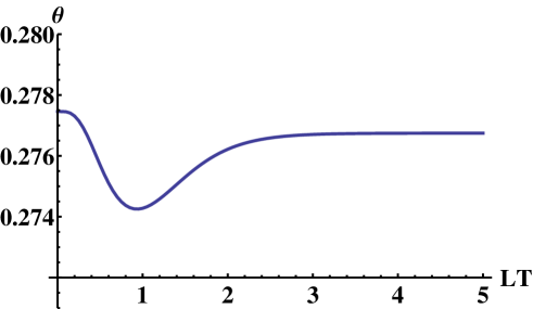
Figure 1: The behavior of $\theta$ with respect to $LT$ in the model (30). The asymptotic value of $\theta$ for $LT\gg 1$ is about $0.276746$, which is consistent with the one obtained from the four-dimensional gauge theory explained in the text.

We do not find the vacuum configuration that respects the $SU(2)$ gauge symmetry for any values of $LT$. This means that, even if we go to the high temperature, the gauge symmetry is not restored, unlike the usual Higgs mechanism. Hence, the model realizes the symmetry nonrestoration. At high temperature, $LT\gg 1$, we find that the vacuum expectation value approaches

$$\theta\simeq 0.276746.$$ (32)

We also observe that the model does not have a phase transition.

As discussed in the previous section, at high temperature, $LT\gg 1$, $\theta$ is determined by a four-dimensional $(R^{3}\times S_{L}^{1})$ gauge theory including the bosonic degrees of freedom alone. In the high temperature limit, the present model (30) consists of the gauge, adjoint and fundamental scalar fields. The vacuum expectation value $\theta$ of the four-dimensional gauge theory is numerically found to be $\theta\simeq 0.276746$, which is the same as (32) obtained by the original five-dimensional gauge theory in the high temperature limit.

Let us next present a model with the inverse symmetry breaking. The matter content in this case is given by

$$\left(N_{fd}^{s},~{}\alpha\right)=\left(1,~{}{1\over 2}\right),\left(N_{adj}^{s},~{}\alpha\right)=\left(5,~{}{1\over 2}\right),\left(N_{fd}^{f},~{}\alpha\right)=\left(1,~{}0\right),\left(N_{adj}^{f},~{}\alpha\right)=\left(0,~{}0\right).$$ (33)

The notations are the same as before. Let us note again that we consider the scalars satisfying the antiperiodic boundary condition.

At zero temperature, $LT=0$, the vacuum configuration of the model is found to be

$$\theta=0.5,$$ (34)

for which the $SU(2)$ gauge symmetry is unbroken. Let us note that the massless gauge boson exists in the spectrum even for the nontrivial value (34). When we turn on and increase the temperature, the vacuum expectation value $\theta$ changes as depicted in Fig.$2$

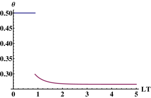
Figure 2: The behavior of $\theta$ with respect to $LT$ in the model (33). The critical temperature, at which the vacuum expectation value jumps, is $LT_{c}\simeq 0.8836$. The asymptotic value of $\theta$ is about $0.265649$, which is consistent with the value obtained by the four-dimensional gauge theory explained in the text.

We observe that the value of $\theta$ jumps at the critical temperature $LT_{c}\simeq 0.8836$, and the degenerate vacuum configurations—one is $\theta=0.5$, and the other is $\theta\simeq 0.298456$—appear. The latter configuration breaks the $SU(2)$ gauge symmetry down to $U(1)$. The asymptotic value for $LT\gg 1$ is

$$\theta\simeq 0.265649.$$ (35)

The $SU(2)$ gauge symmetry is not restored. Hence, the model realizes the inverse symmetry breaking. We also depict the behavior of the effective potential at around the critical temperature in Fig. $3$. The phase transition is clearly first order, which is also understood from the discontinuity of the vacuum expectation value in Fig. $2$.

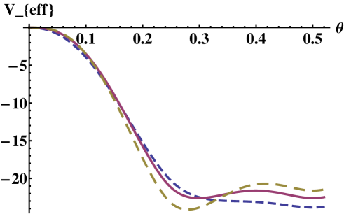
Figure 3: The behavior of the effective potential with respect to $LT$ in the model (33). The solid (dashed, dotted) line corresponds to $LT=LT_{c}(1.2,0.5)$, respectively. The critical temperature $LT_{c}$ is about $0.8836$. The potential is symmetric with respect to $\theta=0.5$, as understood from (28) and (29).

At high temperature, $LT\gg 1$, the $\theta$ is determined by a four-dimensional $(R^{3}\times S_{L}^{1})$ gauge theory, where all of the fermions are decoupled and the Euclidean time coordinate shrinks. The $\theta$ in the four-dimensional gauge theory is numerically found to be $\theta\simeq 0.265649$. This is the same as (35) obtained by the original five-dimensional gauge theory at the high temperature limit.

We have presented the models with the symmetry nonrestoration and the inverse symmetry breaking at high temperature. We note that at high temperature the model is described by the four-dimensional $(R^{3}\times S_{L}^{1})$ gauge theory including only bosonic degrees of freedom. The nontrivial boundary condition $\alpha$ for the scalar fields is crucial for the two interesting phenomena at high temperature.

Let us finally present a model which has both the usual symmetry restoration of the $SU(2)$ gauge symmetry and the inverse symmetry breaking in the intermediate range of $LT$. The matter content is given by

$$\left(N_{fd}^{s},~{}\alpha\right)=\left(2,~{}{1\over 2}\right),\left(N_{adj}^{s},~{}\alpha\right)=\left(6,~{}{1\over 2}\right),\left(N_{fd}^{f},~{}\alpha\right)=\left(1,~{}0\right),\left(N_{adj}^{f},~{}\alpha\right)=\left(0,~{}0\right).$$ (36)

The vacuum configuration at zero temperature is numerically found to be

$$\theta\simeq 0.359407,$$ (37)

for which the $SU(2)$ gauge symmetry is broken to $U(1)$. If we increase the temperature, the behavior of the vacuum expectation value $\theta$ with respect to $LT$ is given in Fig. $4$.

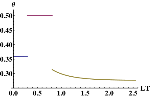
Figure 4: The behavior of $\theta$ respect to $LT$ in the model (36). The first (second) jump of the vacuum expectation value occurs at $LT\simeq 0.2914(0.8104)$. The asymptotic value for $LT\gg 1$ is about $0.276746$, which is consistent with the one obtained by the four-dimensional gauge theory explained in the text.

The first order phase transition occurs at $LT_{c1}\simeq 0.2914$, and the $SU(2)$ gauge symmetry is restored like the usual Higgs mechanism. The second phase transition, which is again first order, occurs at $LT_{c2}\simeq 0.8104$. The $SU(2)$ gauge symmetry is again broken to $U(1)$ at high temperature. The asymptotic value for $LT\gg 1$ is $\theta\simeq 0.276747$. This model belongs to the class of the inverse symmetry breaking at high temperature, but the model has the usual symmetry restoration of the $SU(2)$ gauge symmetry in the intermediate range of the temperature. This is similar to the phase transition discussed in [30].

6 Conclusions

We have investigated the $D$-dimensional gauge theory with an extra dimension of a circle, in particular at high and low temperature. The theory possesses two order parameters of gauge symmetry breaking: One is the zero mode of the gauge field for the Euclidean time direction and the other is that for the direction of the extra dimension. We have evaluated the effective potential for the order parameters in the one-loop approximation and succeeded in expressing it in three different forms: One is suitable for high temperature/large extra dimension, another is suitable for low temperature/a small extra dimension, and the third one is useful for numerical computations. Using those expressions and mainly focusing on the expectation value $\langle a_{y}\rangle$ of the extra component of the gauge field, we have found that at high temperature the effective potential for $\langle a_{y}\rangle$ in the $D$-dimensional gauge theory on the circle reduces to that in a $(D-1)$-dimensional theory defined by removing the Euclidean time coordinate and all of the fermions from the original theory, while at low temperature it is determined by the original $D$-dimensional gauge theory on the circle at zero temperature. This result leads to the conclusion that the gauge symmetry nonrestoration and/or the inverse symmetry breaking at high temperature can occur in a class of gauge theories on a circle with appropriate matter contents.

As a demonstration, we have presented $5d~{}SU(2)$ gauge models on a circle that cause the gauge symmetry nonrestoration or the inverse symmetry breaking to indeed occur at high temperature. Those properties should be contrasted to the gauge symmetry breaking induced by the Higgs mechanism. In this case, one-loop radiative corrections to the Higgs mass squared will be proportional to $T^{2}$ with positive coefficients at high temperature, so that the gauge symmetry is expected to be restored at high temperature [15, 16, 17]. We have further discussed that phase transitions in such a class of gauge theories are, in general, first order and have shown that it is actually the case for the models we have studied.

Considering the higher rank gauge group such as $SU(3)$ is one of the simplest extensions of our studies. There are more symmetry breaking patterns through $\langle a_{y}\rangle$ for that case than the case of $SU(2)$. We expect a rich variety of vacuum structure at finite temperature [32].

We can also easily extend the expressions of (22) and (26) to gauge theories with extra dimensions of a higher-dimensional tori $T^{p}=S_{L_{1}}^{1}\times S_{L_{2}}^{1}\times\cdots\times S_{L_{p}}^{1}$. Then the one-loop effective potential can be expressed in the following two ways:

$$V^{D}(\langle a_{\tau}\rangle,\beta;\langle a_{y_{i}}\rangle,L_{i},\alpha_{i};M)_{\cal R} = V^{D}(\langle a_{\tau}\rangle,\beta;M)_{\cal R}+{1\over\beta}\sum_{{\tilde{l}}=-\infty}^{\infty}V^{D-1}(\langle a_{y_{i}}\rangle,L_{i},\alpha_{i};M_{\tilde{l}})_{\cal R}$$ (38)

$$= V^{D}(\langle a_{y_{i}}\rangle,L_{i},\alpha_{i};M)_{\cal R}$$

$$+{1\over L_{1}\cdots L_{p}}\sum_{{\tilde{n}}_{1},\cdots,{\tilde{n}}_{p}=-\infty}^{\infty}V^{D-p}(\langle a_{\tau}\rangle,\beta;M_{{\tilde{n}}_{1}\cdots{\tilde{n}}_{p}})_{\cal R},$$

where

$$M_{{\tilde{n}}_{1}\cdots{\tilde{n}}_{p}}\equiv\sqrt{M^{2}+\sum_{i=1}^{p}\left({2\pi\over L_{i}}\right)^{2}({\tilde{n}}_{i}+\langle a_{y_{i}}\rangle+\alpha_{i})^{2}}.$$ (39)

It immediately follows that at high temperature the vacuum configuration for $\langle a_{y_{i}}\rangle(i=1,\cdots,p)$ can be determined by the $(D-1)$-dimensional (zero temperature) gauge theory on the tori $T^{p}$ without fermions, while at low temperature it can be determined by the original $D$-dimensional zero temperature gauge theory on $T^{p}$, so that the gauge symmetry nonrestoration and/or the inverse symmetry breaking at high temperature can occur in a class of gauge theories compactified on $T^{p}$.

We would like to make some comments on high and low temperature approximations and also higher order effects. We have shown that the one-loop effective potential (17) can be written into the two other different forms (22) and (26). The expression (22) ((26)) is useful for the analysis at high (low) temperature $LT\gg 1$ ($LT\ll 1$) because contributions of the nonzero Matsubara (Kaluza-Klein) modes are exponentially suppressed. Those modes, however, become important at $LT\approx 1$, and high (low) temperature approximations will break down. Then the analyses of the one-loop effective potential at $LT\approx 1$ may be performed by numerical computations with the original expression (17). The above observation suggests that a phase transition will occur at a critical temperature $T_{c}$ of order $1/L$ if the high temperature vacuum configuration is different from the low temperature one. This has been confirmed for the models studied in the section $5$.

Our considerations are restricted to the one-loop approximation. Higher order effects could alter one-loop results. One such effect will be temperature-dependent mass corrections. At two-loop order, the squared mass $M_{\tilde{l}}^{2}$ of the Matsubara mode ${\tilde{l}}$ could acquire a mass correction $\Delta M^{2}\sim g^{2}T^{3}$ . Then $M_{\tilde{l}}$ in (21) is expected to be replaced by $\sqrt{M_{\tilde{l}}^{2}+\Delta M^{2}}$. If $\sqrt{\Delta M^{2}}L\gg 1$, i.e. $LT\gg 1/(g_{4}^{2})^{1/3}$, where $g_{4}^{2}\equiv g^{2}/L$ is a $4d$ dimensionless coupling constant, contributions of all of the bosonic modes would be exponentially suppressed like fermionic ones. Therefore, for such a high temperature region, higher order effects should be considered properly.

Our results suggest that if the gauge symmetry breaking was caused not by Higgs fields but by gauge fields of extra dimensions, the gauge symmetry could not be restored at the early Universe or the gauge symmetry could be restored with the first order phase transition. It would be of great importance to investigate cosmological implications in such a scenario.

Acknowledgement

This work is supported in part by a Grant-in-Aid for Scientific Research (No. 18540275 (M.S.) and No. 21540285 (K.T.)) from the Japanese Ministry of Education, Science, Sports and Culture. The authors thank Y. Hosotani, T. Inagaki, Y. Kikukawa, T. Onogi, H. So, H. Sonoda and H. Yoneyama for valuable discussions.

References

- [1] M. S. Manton, Nucl. Phys. B158, 141 (1979).
- [2] D. B. Fairlie, Phys. Lett. B82, 97 (1979).
- [3] J. Scherk and J. Schwarz, Phys. Lett. B82, 60 (1979); Nucl. Phys. B153, 61 (1979).
- [4] Y. Hosotani, Phys. Lett. B126, 309 (1983), Ann. Phys. (N.Y.) 190, 233 (1989).
- [5] C. Csaki, C. Grojean, H. Murayama, L. Pilo and J. Terning, Phys. Rev. D69, 055006 (2004).
- [6] M. Sakamoto, M. Tachibana and K. Takenaga, Phys. Lett. B458, 231 (1999); Prog. Theor. Phys. 104, 633 (2000).
- [7] M. Sakamoto, M. Tachibana and K. Takenaga, Phys. Lett. B457, 33 (1999).
- [8] S. Matsumoto, M. Sakamoto and S. Tanimura, Phys. Lett. B518, 163 (2001); M. Sakamoto and S. Tanimura, Phys. Rev. D65, 065004 (2002).
- [9] H. Hatanaka, K. Ohnishi,M. Sakamoto and K. Takenaga, Prog. Theor. Phys. 107, 1191 (2002), Prog. Theor. Phys. 110, 791 (2003).
- [10] K. Ohnishi and M. Sakamoto, Phys. Lett. B486, 179 (2000); H. Hatanaka, S. Matsumoto, K. Ohnishi and M. Sakamoto, Phys. Rev. D63, 105003 (2001).
- [11] L. Randall and R. Sundrum, Phys. Rev. Lett. 83, 4690 (1999).
- [12] H. Hatanaka, M. Sakamoto, M. Tachibana and K. Takenaga, Prog. Theor. Phys. 102, 1213 (1999).
- [13] T. Nagasawa and M. Sakamoto, Prog. Theor. Phys. 112, 629 (2004).
- [14] M. Sakamoto and K. Takenaga, Phys. Rev. D75, 045015 (2007).
- [15] D. A. Kirzhnits, A. Linde, Phys. Lett. B42, 471 (1972).
- [16] L. Dolan and R. Jackiw, Phys. Rev. D9, 3320 (1974).
- [17] S. Weinberg, Phys. Rev. D9, 3357 (1974).
- [18] R. Mohapatra and G. Senjanovic, Phys. Rev. Lett. 42, 1651 (1979); Phys. Rev. D20, 3390 (1979); G. R. Dvali, A. Melfo and G. Senjanovic; Phys. Rev. Lett. 75, 4559 (1995); G.R. Dvali and K. Tamvakis, Phys. Lett. B378, 141 (1996); G. Bimonte and G. Lozano, Nucl. Phys. B460, 155 (1996), M. B. Pinto and R. O. Ramos, Phys. Rev. D61, 125016 (2000); M. B. Pinto, R. O. Ramos and J. E. Parreira, Phys. Rev. D71, 123519 (2005).
- [19] D. J. Gross, R. D. Pisarski and L. G. Yaffe, Rev. Mod. Phys. 53, 43 (1981).
- [20] M. Sakamoto and K. Takenaga, Phys. Rev. D76, 085016 (2007).
- [21] N. Weiss, Phys. Rev. D24, 475 (1981), Phys. Rev. D25, 2667 (1982).
- [22] C. P. Korthals and M. Laine, Phys. Lett. B511, 269 (2001).
- [23] K. Farakos and P. Pasipoularides, Nucl. Phys. B705, 92 (2005).
- [24] N. Maru and K. Takenaga, Phys. Rev. D72, 046003 (2005); Phys. Rev. D74, 015017 (2006).
- [25] A. Delgado, A. Pomarol and M. Quiros, Phys. Rev. D60, 095008 (1999).
- [26] K. Takenaga, Phys. Lett. B570, 244 (2003).
- [27] H. Hata and T. Kugo, Phys. Rev. D21, 3333 (1980).
- [28] P. H. Ginsparg, Nucl. Phys. B170, 388 (1980).
- [29] E. Braaten and A. Nieto, Phys. Rev. D51, 6990 (1995).
- [30] J. R. Espinosa, M. Losada and A. Riotto, Phys. Rev. D72, 043520 (2005).
- [31] A. T. Davies and A. McLachlan, Nucl. Phys. B317, 237 (1989), A. McLachlan, Nucl. Phys. B338, 188 (1990), J. E. Hetrick and C. L. Ho, Phys. Rev. D40, 4085 (1989), C. L. Ho and Y. Hosotani, Nucl. Phys. B345, 445 (1990), A. McLachlan, Nucl. Phys. B338, 188 (1990), H. Hatanaka, Prog. Theor. Phys. 102, 407 (1999), K. Takenaga, Phys. Lett. B425, 114 (1998); Phys. Rev. D58, 026004 (1998); 66 085009 (2002); Phys. Lett. B570, 244 (2003); N. Haba, K. Takenaga and T. Yamashita, Phys. Lett. B605, 355 (2005).
- [32] M. Sakamoto and K. Takenaga (work in progress).