Estimators for CMB statistical anisotropy

Abstract

We use quadratic maximum-likelihood (QML) estimators to constrain models with Gaussian but statistically anisotropic Cosmic Microwave Background (CMB) fluctuations, using CMB maps with realistic sky-coverage and instrumental noise. This approach is optimal when the anisotropy is small, or when checking for consistency with isotropy. We demonstrate the power of the QML approach by applying it to the WMAP data to constrain several models which modulate the observed CMB fluctuations to produce a statistically anisotropic sky. We first constrain an empirically motivated spatial modulation of the observed CMB fluctuations, reproducing marginal evidence for a dipolar modulation pattern with amplitude $7\%$ at $l\lesssim 60$, but demonstrate that the effect decreases at higher multipoles and is $\lesssim 1\%$ at $l\sim 500$. We also look for evidence of a direction-dependent primordial power spectrum, finding a very statistically significant quadrupole signal nearly aligned with the ecliptic plane; however we argue this anisotropy is largely contaminated by observational systematics. Finally, we constrain the anisotropy due to a spatial modulation of adiabatic and isocurvature primordial perturbations, and discuss the close relationship between anisotropy and non-Gaussianity estimators.

I Introduction

The temperature fluctuations of the Cosmic Microwave Background (CMB) are often assumed to be a realization of a statistically isotropic Gaussian random field. Decomposing the temperature fluctuations $\Theta(\Omega)$ into harmonic coefficients

$$\Theta_{lm}=\int{\rm d}\Omega Y_{lm}^{*}(\Omega)\Theta(\Omega),$$ (1)

the covariance of the CMB is then given by $C_{lm,l^{\prime}m^{\prime}}=\langle\Theta_{lm}\Theta^{*}_{l^{\prime}m^{\prime}}\rangle=\delta_{ll^{\prime}}\delta_{mm^{\prime}}C_{l}^{\Theta\Theta}$, and the statistical properties of the fluctuations are completely described by the power spectrum $C^{\Theta\Theta}_{l}$. The assumption of statistical isotropy is well motivated theoretically, both as an application of the Copernican principle and as a prediction of more detailed cosmological models such as inflation. It is a central tenet of modern precision cosmology and the standard $\Lambda$CDM model, and as such needs to be rigorously tested. There are already tantalizing hints in the WMAP data for violation of statistical isotropy, for example alignments of low multipoles Tegmark et al. (2003); Bielewicz et al. (2004); Copi et al. (2006), the axis of evil Land and Magueijo (2005), power asymmetries Eriksen et al. (2004); Hansen et al. (2008), and the cold spot Cruz et al. (2007). Many of these oddities have been discovered in the absence of a proposed model, and so the degree of a posteriori bias which they are subject to is difficult to assess.

In this paper, we will discuss estimators which can be used to constrain the parameters of many CMB models which are Gaussian but perturbatively anisotropic, such that the covariance contains small off-diagonal elements. There are many good reasons to consider such models. Secondary effects that are linear in the CMB temperature result in a guaranteed signal of this form at the ${\cal O}(10^{-3})$ level: gravitational lensing Lewis and Challinor (2006), patchy reionization Dvorkin and Smith (2009) and the doppler shifting due to the motion of our frame relative to the CMB, for example, may be thought of in this context and should become observable with the upcoming generation of CMB measurements. Many non-linear effects and non-standard models can be considered as a fixed modulation of an initially Gaussian field, which is still Gaussian but anisotropic if the modulation is considered fixed. More speculatively, recently proposed anisotropic models of inflation could lead to primordial fluctuations that are anisotropic Gumrukcuoglu et al. (2007); Ackerman et al. (2007). A non-zero primordial bispectrum can also be considered in this framework, where there is a power anisotropy correlated to the temperature, although the current data indicates that any non-Gaussianity consistent with the expectations from inflationary models is small. Models of modulated pre-heating Bond et al. (2009), inflationary bubble collisions (e.g. Chang et al. (2009)), topological defects (e.g. Cruz et al. (2008)), and various other interesting scenarios could also give observable effects that may show up in simple anisotropy estimators motivated by Gaussian anisotropic models, although the signature would typically not be Gaussian in these cases. In the case that the CMB is actually isotropic, the estimators which we will discuss simply place optimal, minimum-variance constraints on the degree of anisotropy, and hence provide valuable tests of consistency and systematics.

Assuming that the instrumental noise is also Gaussian, the rigorous approach to an analysis of these models is clear: calculate the log-likelihood ${\cal L}$ of the observed CMB, given by

$$-{\cal L}(\mathbf{\hat{\Theta}}|\mathbf{h})=\frac{1}{2}\mathbf{\hat{\Theta}}^{{\dagger}}(\bm{C}^{\hat{\Theta}\hat{\Theta}})^{-1}\mathbf{\hat{\Theta}}+\frac{1}{2}\ln\det(\bm{C}^{\hat{\Theta}\hat{\Theta}}),$$ (2)

where $\mathbf{h}$ are parameters characterizing the anisotropy, $\mathbf{\hat{\Theta}}$ is the observed CMB and $\bm{C}^{\hat{\Theta}\hat{\Theta}}\equiv\bm{C}^{\Theta\Theta}+\bm{C}^{NN}$ is its covariance, incorporating the theoretical (anisotropic) covariance as well as instrumental noise. For modern datasets with hundreds of thousands of modes, the full covariance matrix $\bm{C}^{\hat{\Theta}\hat{\Theta}}$ is unmanageably large. To work with it directly therefore requires either artificial limitation of the analysis to some subset of the data Gordon (2007); Hoftuft et al. (2009), or exploitable sparseness Groeneboom and Eriksen (2009). In this work, we will take a quadratic estimator approach, expanding the likelihood to low order in the anisotropy. This approach is not a new one: it was originally used for the purpose of lens reconstruction by Ref. Hirata and Seljak (2003), and many of the estimators that we will discuss here have also been derived for full-sky coverage as minimum-variance estimators with quadratic form Dvorkin et al. (2008); Dvorkin and Smith (2009); Pullen and Kamionkowski (2007); Armendariz-Picon (2006); Prunet et al. (2005). In this paper we will generalize these estimators for application to real data, and show that in special cases where it is actually feasible to perform the more computationally intensive exact-likelihood analysis the quadratic approach produces effectively identical results.

Although we will frame our discussion here on Gaussian but statistically anisotropic models, we note that every statistically anisotropic Gaussian model is related to a statistically isotropic but non-Gaussian model: if there is a preferred direction, taking the direction as being a random variable (e.g. by a random rotation) makes the distribution statistically isotropic at the expense of complicating the statistics. In the statistically isotropic interpretation the anisotropy estimators we discuss would always have zero expectation, but the non-zero disconnected four-point function gives the estimators a variance above that expected for a Gaussian isotropic field, giving an equivalent means of detection. This interpretation is particularly useful for e.g. lens reconstruction and patchy reionization, where the particular realization of the anisotropy, as constrained by the likelihood estimator, is sometimes of less interest than its statistics, contained in the power spectrum of the estimates.

We shall focus on the CMB temperature, since this is measured with much lower noise than the polarization, especially on smaller scales. However if there is significant evidence for anisotropy, polarization information would ultimately be an excellent way to further constrain the origin of the signal: an anisotropic power spectrum at recombination for example, should give a consistent signal in the polarization, but if the signal is local – e.g. due to an unknown foreground or instrumental systematic – the polarization signal could be quite different. The generalization of these estimators to the polarized case is in principle straightforward.

II Anisotropy estimators

We begin by introducing the methodology of anisotropy estimation as a likelihood maximization, loosely following Hirata and Seljak who pioneered this approach for CMB lensing Hirata and Seljak (2003).

Differentiating the likelihood of Eq. (2) with respect to a set of parameters $\mathbf{h}$ which characterize the anisotropy gives

$$\frac{\delta{\cal L}}{\delta\mathbf{h}^{\dagger}} = -\frac{1}{2}\mathbf{\hat{\Theta}}^{\dagger}(\bm{C}^{\hat{\Theta}\hat{\Theta}})^{-1}\frac{\delta\bm{C}^{\hat{\Theta}\hat{\Theta}}}{\delta\mathbf{h}^{\dagger}}(\bm{C}^{\hat{\Theta}\hat{\Theta}})^{-1}\mathbf{\hat{\Theta}}$$ (3)

$$+\frac{1}{2}\mathbf{{\rm Tr}}\left[(\bm{C}^{\hat{\Theta}\hat{\Theta}})^{-1}\frac{\delta\bm{C}^{\hat{\Theta}\hat{\Theta}}}{\delta\mathbf{h}^{\dagger}}\right].$$

The trace term results in a “mean field” over realizations of the observed CMB. To see this, consider the identity ${\rm Tr}(\bm{A})=\langle\mathbf{x}^{\dagger}\bm{A}\bm{C}^{-1}\mathbf{x}\rangle$, where $\bm{A}$ is any matrix and $\mathbf{x}$ is a vector of Gaussian random variables with covariance $\bm{C}$. Making this substitution with $\bm{C}=\bm{C}^{\hat{\Theta}\hat{\Theta}}$ and maximizing the likelihood by setting $\delta{\cal L}/\delta\mathbf{h}^{\dagger}=0$ gives the simple equation

$$\frac{\delta{\cal L}}{\delta\mathbf{h}^{\dagger}}=\left<\bm{{\cal H}}\right>-\bm{{\cal H}}=0,$$ (4)

where

$$\bm{{\cal H}}=\frac{1}{2}\left[(\bm{C}^{\hat{\Theta}\hat{\Theta}})^{-1}\mathbf{\hat{\Theta}}\right]^{{\dagger}}\frac{\delta\bm{C}^{\hat{\Theta}\hat{\Theta}}}{\delta\mathbf{h}^{\dagger}}\left[(\bm{C}^{\hat{\Theta}\hat{\Theta}})^{-1}\mathbf{\hat{\Theta}}\right].$$ (5)

The maximum-likelihood (M-L) point can be determined iteratively using Newton’s method

$$\mathbf{h}_{i+1}=\mathbf{h}_{i}-\left[\left.\frac{\delta}{\delta\mathbf{h}^{\dagger}}(\left<\bm{{\cal H}}\right>-\bm{{\cal H}})^{\dagger}\right|^{\dagger}_{i}\right]^{-1}(\left<\bm{{\cal H}}\right>_{i}-\bm{{\cal H}}_{i}),$$ (6)

where quantities subscripted with $i$ are evaluated for the estimate $\mathbf{h}_{i}$ of the $i^{\rm th}$ iteration. Note that Eq. (6) is a very general way to maximize a Gaussian likelihood when the covariance is perturbatively linear in a set of parameters. It leads to the power spectrum estimator of Ref. Tegmark (1997), for example, if one takes the $\mathbf{h}$ parameters to encode the CMB power spectrum. We shall assume that the noise and normal cosmological parameters are known, so we are only maximizing the anisotropy parameters; if the assumed parameters (and hence isotropic power spectrum) are incorrect this could lead to small biases in the estimator.

We are working under the assumption that any anisotropy which we will be studying is “weak”, and so a single iteration of Eq. (6), starting from $\mathbf{h}=\mathbf{0}$ should give a sufficiently accurate estimate of $\mathbf{h}$. For simplicity, the derivative term is replaced with its ensemble average

$$\left<\frac{\delta}{\delta\mathbf{h}^{\dagger}}(\left<\bm{{\cal H}}\right>-\bm{{\cal H}})^{\dagger}\right> = \left<\frac{\delta}{\delta\mathbf{h}^{\dagger}}\frac{\delta{\cal L}}{\delta\mathbf{h}}\right>$$ (7)

$$= \left<\frac{\delta{\cal L}}{\delta\mathbf{h}^{\dagger}}\frac{\delta{\cal L}}{\delta\mathbf{h}}\right>$$

$$= \left[\left<\bm{{\cal H}}\bm{{\cal H}}^{{\dagger}}\right>-\left<\bm{{\cal H}}\right>\left<\bm{{\cal H}}\right>^{{\dagger}}\right]$$

$$= \bm{{\cal F}},$$

where the equality between the second and third lines is dictated by the normalization of the likelihood and $\bm{{\cal F}}$ is the Fisher matrix, considering the likelihood to be a function of the parameters $\mathbf{h}$. Putting all of this together, we have an approximate, quadratic maximum-likelihood (QML) estimator of the form

$$\mathbf{\hat{h}}=\bm{{\cal F}}^{-1}[\mathbf{\tilde{h}}-\langle\mathbf{\tilde{h}}\rangle].$$ (8)

The inverse Fisher matrix can be thought of as the estimator normalization, as well as its covariance in the limit of no anisotropy. The quadratic part of the estimator is given by

$$\mathbf{\tilde{h}}=\bm{{\cal H}}_{0} = \frac{1}{2}\mathbf{\bar{\Theta}}^{\dagger}\frac{\delta\bm{C}^{\hat{\Theta}\hat{\Theta}}}{\delta\mathbf{h}^{\dagger}}\mathbf{\bar{\Theta}}$$ (9)

$$= \frac{1}{2}\sum_{lm,l^{\prime}m^{\prime}}\left[\frac{\delta C^{\hat{\Theta}\hat{\Theta}}_{lm,\ l^{\prime}m^{\prime}}}{\delta\mathbf{h}^{\dagger}}\right]\bar{\Theta}^{*}_{lm}\bar{\Theta}_{l^{\prime}m^{\prime}},$$

where $\mathbf{\bar{\Theta}}=(\bm{C}^{\hat{\Theta}\hat{\Theta}})^{-1}|_{0}\mathbf{\hat{\Theta}}$ is the observed sky after application of inverse-variance filtering with $\mathbf{h}=\mathbf{0}$. In the limit of weak anisotropy this QML estimator saturates the Cramer-Rao inequality, and so is optimal in the minimum-variance sense. In practice, “weak” means non-detection, and so this form of quadratic estimator is excellent for testing statistical isotropy, but needs to be treated with care if a significant detection is made (as is soon expected to be the case, for example, with CMB lensing). In this work we have occasion to compare some of our results to exact likelihood calculations by other authors, and find good agreement.

Thus, the QML formalism makes it straightforward to construct estimators for any form of Gaussian but statistically anisotropic model which is accurately parameterized as a linear function of a set of parameters $\mathbf{h}$. To assess the significance of a possible detection, a useful statistic is the $\chi^{2}$ value of the estimate, given by

$$\chi^{2}(\hat{\mathbf{f}})=\hat{\mathbf{f}}^{{\dagger}}\bm{{\cal F}}\hat{\mathbf{f}}.$$ (10)

For $n$ constrained parameters, the measured value can be compared to the cumulative distribution function (CDF) of the $\chi^{2}_{n}$ distribution to produce an intuitive “p-value” figure of merit, which for this paper we will define to be the probability of attaining a greater value of $\chi^{2}$ in an isotropic model.

There are several advantages of the quadratic approach:

• Speed: Provided that an inverse variance filtered sky-map has already been calculated, the evaluation of the $\tilde{h}$ terms is at most ${\cal O}(l_{\rm max}^{4})$. In practice, the QML approach often results in estimators which have a fast implementation in real space, making them ${\cal O}(l_{\rm max}^{3})$. Simulations are often required to determine the mean-field and estimator normalization, but the number of these is generally less than are needed for an exploration of the likelihood.

  In many situations, QML estimators also enable the study of a much larger model space than could conceivably be explored with exact likelihood evaluations. For example, the modulation anisotropy models which we will use in the following sections result in QML estimators which produce an entire modulation sky-map, rather than just estimating a small number of its coefficients as has been done in previous exact likelihood analyses. This can help to identify the source of contaminating signals.

• Systematic and jacknife tests: The quadratic estimator approach is amenable to certain systematic and jacknife tests for which there are no analogues in an exact likelihood exploration. The effects of correlated noise, for example, can be avoided straightforwardly by forming the anisotropy estimates from cross-correlations between maps with different noise realizations. In this case, the likelihood approach which was used to derive our estimator is invalid. In particular, the estimator normalization and the reconstruction covariance are no longer equal. For full-sky coverage and homogeneous noise they may be derived using a minimum-variance approach, similar to that which is used in Ref. Okamoto and Hu (2003). For the purpose of significance testing however, it is irrelevant whether the estimates are properly normalized, only that their covariance is accurately characterized. The $\chi^{2}$ value defined in Eq. (10), for example, is still a valid measure of significance, even though the inverse Fisher matrix no longer properly normalizes the estimates.

  The quadratic approach also enables the use of simple jacknife tests in harmonic space. The sum of Eq. (9), for example, can be broken up into contributions from different multipole ranges at no additional computational cost. Provided that the inverse variance filter does not significantly mix the modes of the observed CMB across the chosen multipole ranges, this can be used to construct anisotropy estimators in bands, and localize the origin of any detected anisotropy in harmonic space.

  In the quadratic approach the treatment of additional Gaussian but anisotropic systematics is also clear. Provided that such effects can be incorporated into the simulation and inverse-variance filtering steps they will be subtracted from the anisotropy estimates and their additional contribution to the variance of the estimates will be included in ${\cal F}^{-1}$. The effect of beam asymmetries and sidelobe pickup, for example, fall neatly into this category, though a method for correcting the contaminating signals could be better in practice.

We now proceed to apply the QML formalism to several anisotropic modulation models, which we constrain using the WMAP data.

III Implementation

We will test the assumption of statistical anisotropy in the WMAP 5-year maps, which are provided in HEALPix format at $N_{\text{side}}=512$ Hinshaw et al. (2009). Specifically, we will study the Q-, V- and W-band data at $40$, $60$ and $90$Ghz. We limit our analysis of the Q-band data to $l_{\rm max}=300$, as its power spectrum becomes clearly contaminated by point sources at higher multipoles, which we do not attempt to model. The mean field and estimator normalization are generally determined for each data map using Monte-Carlo simulations, although we will sometimes use analytic approximations to the normalization when this is not possible.

For the high-resolution WMAP data, the inverse-variance filtering operation is too costly to perform directly. Instead, we use the conjugate gradients technique to iteratively solve Oh et al. (1999)

$$[(\bm{C}^{\Theta\Theta})^{-1}+\bm{\underline{Y}}^{{\dagger}}\bm{N}^{-1}\bm{\underline{Y}}]\bm{C}^{\Theta\Theta}\mathbf{\bar{\Theta}}=\bm{\underline{Y}}^{\dagger}\bm{N}^{-1}\mathbf{\hat{\Theta}}.$$ (11)

Here $\bm{C}^{\Theta\Theta}$ is the intrinsic CMB covariance, diagonal in harmonic space in the limit of no anisotropy. Throughout this work, we will use a fixed flat $\Lambda$CDM cosmology for $\bm{C}^{\Theta\Theta}$, with standard parameters $\{\Omega_{b},\Omega_{c},h,n_{s},\tau,A_{s}\}=\{0.05,0.23,0.7,0.96,0.08,2.4\times 10^{-9}\}$, which is consistent with the WMAP5 best-fit power spectrum Dunkley et al. (2009). The data itself is contained in the map vector $\mathbf{\hat{\Theta}}$ and $\bm{\underline{Y}}$ is the pointing matrix, which provides the mapping between a harmonic space signal and the observed map:

$$\underline{Y}_{i,(lm)}=B_{l}Y_{lm}(i),$$ (12)

where $B_{l}$ is the transfer function for the beam, which is assumed to be symmetric. Finally, $\bm{N}^{-1}$ is the noise model, which we take in real space to be

$$\bm{N}^{-1}=\bm{N}^{-1}_{\rm pix}-\bm{N}^{-1}_{\rm pix}\bm{T}^{T}[\bm{T}^{T}\bm{N}^{-1}_{\rm pix}\mathbf{T}]^{-1}\mathbf{T}\bm{N}_{\rm pix}^{-1}.$$ (13)

Here $\bm{N}^{-1}_{\rm pix}$ is the covariance matrix of the map noise, which is taken to be uncorrelated between pixels. To effect a sky-cut, $\bm{N}^{-1}_{\rm pix}$ is taken to be zero for masked pixels. $\mathbf{T}$ is an $n_{\rm tmpl.}\times n_{\rm pix}$ matrix of template maps to be projected out of the data. Unless otherwise noted, we use this only to project out the four templates corresponding to monopole and dipole modes.

Within the conjugate gradients approach, the solution of Eq. (11) requires careful preconditioning to be fast enough for the large number of Monte-Carlo simulations which we perform. We implement the multigrid preconditioner given by Ref. Smith et al. (2007), which is the fastest to date. For a fractional error of less than ${\cal O}(10^{-6})$ in each mode of the calculated $\mathbf{\bar{\Theta}}$ field, we find that our implementation has a typical cost of ten minutes on a 2GHz processor, evaluated to $l_{\rm max}=1000$ for WMAP noise with a galactic cut.

IV Results

IV.1 Modulation on the sky

A popular form of modulation anisotropy which has been tested in the literature is given by Gordon et al. (2005)

$$\Theta_{f}(\hat{\mathbf{n}})=[1+f(\hat{\mathbf{n}})]\Theta_{f}^{i}(\hat{\mathbf{n}}),$$ (14)

where $\Theta_{f}^{i}(\hat{\mathbf{n}})$ is some intrinsic statistically isotropic CMB temperature, $f(\hat{\mathbf{n}})$ is a modulating field, and the $f$ subscript denotes restriction to some range of angular scales (e.g. $l\leq{l_{\text{max}}}$). The dipole part of $f(\hat{\mathbf{n}})$ has received particular attention since the work of Ref. Hansen et al. (2004), which found evidence for a large-scale hemispherical power asymmetry in the WMAP data. This pathfinding work was followed by more rigorous likelihood analyses Spergel et al. (2006); Gordon (2007); Eriksen et al. (2007), and recently Refs. Hansen et al. (2008); Hoftuft et al. (2009) have extended the analysis to smaller angular scales, arguing for increased detection significance as more data is added. The exact likelihood analysis is currently limited by computational requirements to multipoles $l\leq 80$, but with the QML approximation to the maximum-likelihood estimator no such difficulties arise, so we can extend our analysis to the limit of current observations.

We note that the doppler effect giving the CMB kinematic dipole also results in a dipole modulation of the assumed form, with $f(\hat{\mathbf{n}})=\bm{\beta}\cdot\hat{\mathbf{n}}$. Assuming a small ${\cal O}(10^{-5})$ primordial dipole, $\bm{\beta}$ is expected to have amplitude $0.0012$ in the direction $(l,b)=(260^{\rm o},50^{\rm o})$ of the observed total dipole. This signal should be present on all scales along with an aberration effect which is degenerate with a CMB lensing dipole. Although we will see that this effect is an order of magnitude too small to be observed with WMAP, it should be detected with high significance in the data of the recently launched Planck satellite Challinor and Sollom (2009). Any robust signal detected at a higher level (amplitude $\gg 0.001$) would be an indicator of cosmological statistical anisotropy, or equivalently non-Gaussianity.

The simplest quadratic estimator for the modulation is just $\hat{\Theta}^{2}$ - an estimator of the temperature variance in each pixel. In a statistically isotropic model a map of $\hat{\Theta}^{2}$ should on average have only a monopole, and there should be no structure which is not consistent with noise or CMB fluctuations. The QML estimator that we derive essentially generalizes this to optimally account for noise and cosmic variance.

The temperature moments of Eq. (14) for the modulation anisotropy are given by

$$\Theta_{lm}=\Theta^{i}_{lm}+\sum_{l^{\prime}m^{\prime},l^{\prime\prime}m^{\prime\prime}}\Theta^{i}_{l^{\prime}m^{\prime}}f_{l^{\prime\prime}m^{\prime\prime}}\int d\Omega Y^{*}_{lm}Y_{l^{\prime}m^{\prime}}Y_{l^{\prime\prime}m^{\prime\prime}},$$ (15)

where $l,l^{\prime}$ are restricted to the range of $l$ under consideration. To first order in $f_{lm}$, the resulting covariance is therefore

$$C_{l_{1}m_{1},l_{2}m_{2}}\equiv\langle\Theta_{l_{1}m_{1}}\Theta_{l_{2}m_{2}}^{*}\rangle\\ =\delta_{l_{1}l_{2}}\delta_{m_{1}m_{2}}C_{l_{1}}+\sum_{lm}f_{lm}[C_{l_{1}}+C_{l_{2}}]\int d\Omega Y_{lm}Y^{*}_{l_{1}m_{1}}Y_{l_{2}m_{2}}.$$ (16)

Using Eq. (9) results in a QML estimator constructed from

$$\tilde{h}^{f}_{lm}=\int d\Omega Y_{lm}^{*}\left[\sum_{l_{1}m_{1}}^{l_{\rm max}}\bar{\Theta}_{l_{1}m_{1}}Y_{l_{1}m_{1}}\right]\left[\sum_{l_{2}m_{2}}^{l_{\rm max}}C_{l_{2}}\bar{\Theta}_{l_{2}m_{2}}Y_{l_{2}m_{2}}\right].$$ (17)

On the full sky the expected value depends only on the off-diagonal part of the underlying temperature realization covariance matrix, and is essentially an optimally weighted combination of the bipolar spherical harmonic coefficients introduced in Ref. Hajian and Souradeep (2003). Here we have written it in a form convenient for fast numerical evaluation in terms of real-space fields; in harmonic space it can be written as

$$\tilde{h}^{f}_{lm} = \frac{1}{2}\sum_{l_{1},m_{1},l_{2},m_{2}}(-1)^{m_{1}}\sqrt{\frac{(2l+1)(2l_{1}+1)(2l_{2}+1)}{4\pi}}$$

$${\begin{pmatrix}l&l_{1}&l_{2}\\ 0&0&0\end{pmatrix}}{\begin{pmatrix}l&l_{1}&l_{2}\\ m&-m_{1}&m_{2}\end{pmatrix}}(C_{l_{1}}+C_{l_{2}})\bar{\Theta}_{l_{1}m_{1}}\bar{\Theta}^{*}_{l_{2}m_{2}}.$$

Due to the triangle constraint $|l_{1}-l_{2}|\leq l\leq|l_{1}+l_{2}|$ from the 3-jm symbols, and the constraint that $l+l_{1}+l_{2}$ is even, we see that the dipole part of $\tilde{h}^{f}_{lm}$ is due to the off-diagonal $l_{1},l_{1}+1$ part of the covariance, and similarly the quadrupole part depends on the $l_{1},l_{1}$, and $l_{1},l_{1}+2$ correlations. Note that the estimator is independent of the modulation pattern, amplitude and orientation, so the estimator only needs to be calculated once to recover all multipoles — there is no need to marginalize over all the possible orientations.

The Fisher matrix is determined by the trispectrum of the inverse-variance filtered CMB. The CMB is assumed to be Gaussian and so this consists only of disconnected terms. A useful tool for forecasting is the portion of the Fisher matrix due to the isotropic terms, i.e. those in which any coupling between modes of the observed CMB are taken to be zero (i.e. we ignore the non-diagonal elements of $\bm{C}^{\hat{\Theta}\hat{\Theta}}$ so $C^{\hat{\Theta}\hat{\Theta}}_{ll^{\prime}}\rightarrow\delta_{ll^{\prime}}C^{\rm{tot}}_{l}$). This is given by

$$\left[{\cal F}^{ff}_{\rm iso}\right]_{lm,l^{\prime}m^{\prime}}=\delta_{ll^{\prime}}\delta_{mm^{\prime}}\\ \times\sum_{l_{1},l_{2}}\frac{(2l_{1}+1)(2l_{2}+1)}{8\pi}{\begin{pmatrix}l&l_{1}&l_{2}\\ 0&0&0\end{pmatrix}}^{2}\frac{(C_{l_{1}}+C_{l_{2}})^{2}}{C^{\rm{tot}}_{l_{1}}C^{\rm{tot}}_{l_{2}}}.$$ (18)

The corresponding estimator noise we denote as $N_{l}^{ff}=[{\cal F}^{ff}_{\rm iso}]^{-1}_{ll}$. In practice, for small sky-cuts and roughly homogeneous uncorrelated instrumental noise this is quite a good approximation to the true covariance. For full-sky coverage and homogeneous noise, it is exact. For a cosmic-variance limited reconstruction, $N^{ff}_{l}$ scales with the number of observed modes, as $l_{\rm max}^{-2}$ at high-$l$. For reconstruction of the modulation dipole $f_{1m}$, for example, we find $N^{ff}_{1}\sim 6.24l_{\rm max}^{-2}$.

Figure 1: Pseudo-$C_{l}$ of the $f_{lm}$ reconstruction for the WMAP V-band foreground-reduced data, with KQ85 mask and $l_{\rm max}=64$ (black solid). The full-sky, isotropic normalization was used rather than the actual inverse Fisher matrix. The $[25,75]\%$ (dark gray) and $[5,95]\%$ (light gray) confidence intervals measured from Monte-Carlo simulations are overlaid.

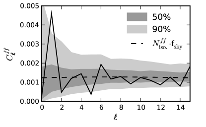
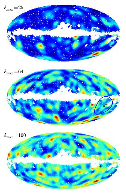
In Fig. 1 we show the pseudo-$C_{l}$ power spectrum of a typical $f_{lm}$ reconstruction. For simplicity we use the isotropic normalization for this plot, with confidence intervals determined by Monte-Carlo simulation. The reconstruction variance compares very well to the full-sky analytical result, scaled by the unmasked sky-fraction. In Fig. 2 we show maps of the reconstructed $f(\hat{\mathbf{n}})$ for $l_{\rm max}=25,\ 64,\ 100$, smoothed with a ten degree beam. The modulation reconstruction brings the hot and cold spots of the observed CMB into sharp relief. The CMB cold spot Cruz et al. (2005), for example, is distinctly visible in all three maps.

Figure 2: Reconstructed maps of $f(\hat{\mathbf{n}})$ for three values of $l_{\rm max}$, smoothed with a ten degree beam. We have used the isotropic normalization for simplicity, which is invalid close to the sky-cut, but works well otherwise. The ‘$+$’ symbols mark the peak of the QML dipole. The ‘$\times$’ symbol and ring in the $l_{\rm max}=64$ plot marks the M-L dipole and error found by Hoftuft et al. (2009), which agrees well with our result.

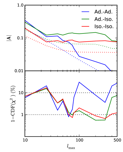
It can be seen from Fig. 1 that the amplitude of the reconstructed modulation is generally in good agreement with that expected from our $\Lambda$CDM simulations, except for the dipole which is slightly high. To make connection with previous work, we will now focus exclusively on the dipole modulation, restricting our reconstruction to the three modes of the dipole, for which we determine the full Fisher matrix by Monte-Carlo. The three dipole modes may be simply related to the amplitude and galactic coordinates of a dot product modulation $f(\hat{\mathbf{n}})=\mathbf{A}\cdot\hat{\mathbf{n}}$. In the upper panel of Fig. 3 we show estimates of this modulation amplitude $|\mathbf{A}|$ for the WMAP data, as well as the expectation value (due to the estimator noise) for a full-sky cosmic variance limited measurement. The observed amplitudes generally lie above the full-sky expectation. This is partially due to the presence of instrumental noise and a sky-cut, particularly at high-$l$ where the WMAP data becomes noise dominated. In the lower panel of Fig. 3 we plot the analytical significance levels of the $\chi^{2}$ values calculated following Eq. (10), given three degrees of freedom. We can see that all of the observed p-values are somewhat low, typically at the five percent significance level. Interestingly, the probability of the observed $f_{1m}$ in an isotropic model is smallest at $l_{\rm max}=40,\ 64$, which are the two most previously studied values.

Figure 3: Summary of modulation dipole results for the foreground-reduced WMAP data. Solid lines correspond to KQ85 masking, and dashed lines use the KQ75 mask. Upper panel: Dipole amplitudes $|\mathbf{A}|$ as a function of the maximum multipole used in the reconstruction. The black dashed line gives the expected value for a cosmic-variance limited experiment, which is non-zero due to the estimator noise. The dotted lines give the reconstruction noise spectra measured from the simulations. They separate into two groups for KQ85 and KQ75 masking and are well described as $f_{\rm sky}^{-1}$ times the ideal result for $l_{\rm max}<300$, but decrease more slowly at higher-$l$ as the instrumental noise becomes non-negligible. Lower panel: $\chi^{2}$ significances of the reconstructions in the isotropic model.

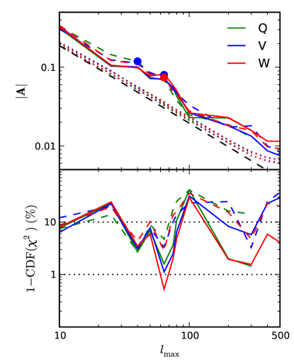
We note that in their region of overlap, our measurements agree well with those of Ref. Hoftuft et al. (2009). Our measured $(A,l,b)$ values for $l_{\rm max}<100$ are all within error of those which they quote, and consistent with a preferred direction of $(l,b)=(225^{\rm o},-22^{\rm o})\pm 24^{\rm o}$. Their quoted significance values also agree well with the square-root of our $\chi^{2}$ values, although we note that for the purposes of testing $\Lambda$CDM, they should be treated as $\chi^{2}_{3}$ significances, rather than Gaussian ones. Fig. 3 shows that the large modulation indicated by the low-$l$ data does not persist on smaller scales however, consistent with the tight constraint on the anisotropy in the quasar distribution Hirata (2009).

Figure 4: Sensitivity of modulation results to various tests, similar to Fig. 3. All data are for WMAP V-band. Blue solid is the V-band foreground-reduced data, with KQ85 mask. Magenta is with the KQ85+CS5 mask. Green is for reconstructions with $l_{\rm min}=20$. Red lines are for raw maps, without template cleaning (solid/dashed correspond to KQ85/KQ75 masking respectively.)

There is still some tension between these measurements of $f_{1m}$ and an isotropic model. Although chance is a possible explanation, it is intriguing that the observed amplitude of dipole modulation is consistently high across a large range of multipole values (although it must be remembered that the measurement of $\mathbf{A}$ is cumulative, and so the estimators at different $l_{\rm max}$ can be strongly correlated). To be rigorous, we consider here several other possible explanations for this tension:

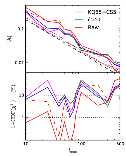
• The cold spot: In Fig. 2 we have seen that the CMB “Cold Spot” Cruz et al. (2005) constitutes a prominent feature in the reconstructed modulation field. It is also close to the dipole of the reconstruction. It is possible that the large dipole amplitude is simply another detection of the Cold Spot. To test this, we perform the modulation reconstruction with a new mask which we call KQ85+CS5, created by augmenting the KQ85 mask with a circular cut of radius five degrees centered at $(l,b)=(208^{\rm o},-56^{\rm o})$. The results of this reanalysis are given in Fig. 4. The removal of the Cold Spot has a large effect for the $l_{\rm max}=25$ reconstruction, but does not significantly effect the reconstructed modulation at higher multipoles.

• Residual low-$l$ anomalies: The modulation model may be motivated as a way to consistently treat the observed low-$l$ power deficit, asymmetry, and alignment issues Spergel et al. (2006). To what extent do the low-$l$ anomalies imprint upon our measurements of $f_{lm}$ for larger values of $l_{\rm max}$? We test this straightforwardly by excluding all of the filtered multipoles below some $l_{\rm min}$ from our analysis. We choose $l_{\rm min}=20$, which ensures that any mixing of the anomalies at $l<10$ due to the sky-cut will have negligible effects on the reconstruction. This is shown in Fig. 4. Again, this excision does not result in any significant reduction of the measured modulation.

• Foregrounds: The consistency of the modulation amplitudes with frequency band and sky-cut makes a foreground explanation for the observed tension seem unlikely. We also confirm that our results are not strongly dependent on the method of foreground subtraction, by marginalizing over the WMAP foreground templates Gold et al. (2009) in the inverse-variance filtering operation, similar to Gordon (2007). Further investigation raises two interesting points, however. To understand the order-of-magnitude for potential foreground effects, we measure the modulation amplitudes for raw WMAP data, without foreground template subtraction. This is plotted in Fig. 4. We can see that complete neglect of foregrounds has a large effect on the estimated modulation. Interestingly, this increase is not strongly dependent on choice of sky-cut, indicating that consistency under changes in the mask size does not represent strong evidence against foreground contamination. Additionally interesting is that the modulation dipole induced by foregrounds is closely aligned with the dipole determined for cleaned maps. In the quadratic estimator approach, an additive template which is uncorrelated with the primary CMB has an additive effect on the reconstructed modulation. The V-band template model, for example, gives a contribution to the dipole of an $l_{\rm max}=40$ analysis in the direction $(l,b)=(208^{\rm o},-10^{\rm o})$, due in roughly equal parts to the contribution from the $H\alpha$ and Finkbeiner dust templates. All of these results are of course for the current foreground model, which is projected out of the data. It seems possible, however, that residual foreground contributions which are morphologically similar may source the tension between the modulation estimates and an isotropic model.

IV.2 Primordial Power Anisotropy

Figure 5: $\sqrt{l(l+1)l_{2}(l_{2}+1)}C_{ll_{2}}/2\pi$ for $a(k)=1$, with $l_{2}=l$ (thick solid), $l_{2}=l+2$ (dashed), $l_{2}=l+4$ (dot-dashed) and $l_{2}=l+20$ (dotted).

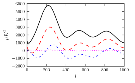
Refs. Ackerman et al. (2007); Gumrukcuoglu et al. (2007); Groeneboom and Eriksen (2009) consider anisotropic models of the early universe, where at late times the universe isotropizes so that the only evidence is an angular-dependent power spectrum on large scales (but isotropic transfer functions). The isotropic real adiabatic transfer functions $\Delta_{l}(k)$ are defined so that

$$\Theta_{lm}=4\pi i^{l}\int\frac{{\rm d}^{3}\mathbf{k}}{(2\pi)^{3}}\Delta_{l}(k)\chi_{0}(\mathbf{k})Y_{lm}^{*}(\hat{\mathbf{k}})$$ (19)

where $\chi_{0}(\mathbf{k})$ is the (statistically anisotropic) primordial perturbation with power spectrum defined by

$$\langle\chi_{0}(\mathbf{k})\chi_{0}^{*}(\mathbf{k}^{\prime})\rangle = (2\pi)^{3}\delta(\mathbf{k}-\mathbf{k}^{\prime})P_{\chi}(\mathbf{k})$$ (20)

$$= (2\pi)^{3}\delta(\mathbf{k}-\mathbf{k}^{\prime})\frac{2\pi^{2}}{k^{3}}\mathcal{P}_{\chi}(\mathbf{k}).$$

The covariance is then given by Gumrukcuoglu et al. (2007)

$$C_{l_{1}m_{1}l_{2}m_{2}}=\\ i^{l_{1}-l_{2}}\frac{\pi}{2}\int{\rm d}^{3}\mathbf{k}P_{\chi}(\mathbf{k})\Delta_{l_{1}}(k)\Delta_{l_{2}}(k)Y_{l_{1}m_{1}}^{*}(\hat{\mathbf{k}})Y_{l_{2}m_{2}}(\hat{\mathbf{k}}).$$ (21)

The anisotropy is contained in the direction-dependent $P_{\chi}(\mathbf{k})$, and we can construct a QML estimator for the angular dependence of the power spectrum at a given $k$ from Eq. (9) using

$$\tilde{h}^{P}_{lm}(k) = \frac{\pi}{2}\int{\rm d}\Omega Y_{lm}^{*}\left[\sum_{l_{1}m_{1}}i^{l_{1}}\Delta_{l_{1}}(k)\bar{\Theta}_{l_{1}m_{1}}Y_{l_{1}m_{1}}\right]$$ (22)

$$\quad\times\left[\sum_{l_{2}m_{2}}i^{-l_{2}}\Delta_{l_{2}}(k)\bar{\Theta}_{l_{2}m_{2}}Y_{l_{2}m_{2}}\right].$$

Refs. Ackerman et al. (2007); Groeneboom and Eriksen (2009); Yokoyama and Soda (2008); Dimopoulos et al. (2009) consider the particularly simple case where the $k$-dependence is in a known function $a(k)$ so that

$$\mathcal{P}_{\chi}(\mathbf{k})=\mathcal{P}_{\chi}(k)[1+a(k)g(\hat{\mathbf{k}})],$$ (23)

and $g(\mathbf{k})=g(-\mathbf{k})$ so $g_{lm}$ has only even-$l$ modes. The covariance in this case is

$$C_{l_{1}m_{1}l_{2}m_{2}}=\delta_{l_{1}l_{2}}\delta_{m_{1}m_{2}}C_{l_{1}}\\ +\sum_{lm}i^{l_{1}-l_{2}}g_{lm}\int{\rm d}\Omega_{\mathbf{k}}C_{l_{1}l_{2}}Y_{lm}Y_{l_{1}m_{1}}^{*}Y_{l_{2}m_{2}}$$ (24)

where

$$C_{l_{1}l_{2}}\equiv 4\pi\int{\rm d}\ln k\mathcal{P}_{\chi}(k)a(k)\Delta_{l_{1}}(k)\Delta_{l_{2}}(k).$$ (25)

The QML estimator for $g$ is therefore constructed from

$$\tilde{h}^{g}_{lm} = \frac{1}{2}\int{\rm d}\Omega Y_{lm}^{*}\sum_{l_{1}l_{2}}i^{l_{1}-l_{2}}C_{l_{1}l_{2}}$$ (26)

$$\quad\times\left[\sum_{m_{1}}\bar{\Theta}_{l_{1}m_{1}}Y_{l_{1}m_{1}}\right]\left[\sum_{m_{2}}\bar{\Theta}_{l_{2}m_{2}}Y_{l_{2}m_{2}}\right].$$

The $i^{l_{1}-l_{2}}$ term forces the reconstruction to zero for odd-$l$. Similar quadratic estimators have been derived before on the full sky Armendariz-Picon (2006); Pullen and Kamionkowski (2007). For a pixelization such as HEALPix  which consists of ${\cal O}(l_{\rm max})$ isolatitude rings, the azimuthal sums may be evaluated using FFTs in ${\cal O}(l_{\rm max}^{2}\log l_{\rm max})$. To estimate $g_{lm}$ to some maximum multipole $\Delta_{l}$, the $C_{l_{1}l_{2}}$ matrix may be treated as band-diagonal with $\Delta_{l}$ bands, due to the triangle constraint on the integral of three spherical harmonics. This leads to a total cost of ${\cal O}(\Delta_{l}l_{\rm max}^{3}\log l_{\rm max})$. An alternative approach is to discretize the integral of Eq. (25), in which case $\hat{g}$ may be evaluated as $n_{k}$ spherical harmonic transforms, where $n_{k}$ is the number of quadrature points for the integral, leading to a cost of ${\cal O}(n_{k}l_{\rm max}^{3})$. A similar technique was applied in Ref. Smith and Zaldarriaga (2006).

The disconnected, isotropic component of the Fisher matrix in this case is given by

$$\left[{\cal F}_{\rm iso}^{gg}\right]_{lm,l^{\prime}m^{\prime}}=\delta_{ll^{\prime}}\delta_{mm^{\prime}}\\ \times\sum_{l_{1},l_{2}}\frac{(2l_{1}+1)(2l_{2}+1)}{8\pi}{\begin{pmatrix}l&l_{1}&l_{2}\\ 0&0&0\end{pmatrix}}^{2}\frac{C_{l_{1}l_{2}}^{2}}{C^{\rm{tot}}_{l_{1}}C^{\rm{tot}}_{l_{2}}}.$$ (27)

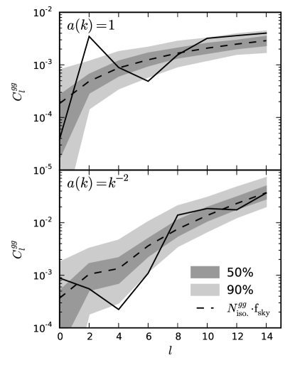
Again we take $N_{l}^{gg}=[{\cal F}^{gg}_{\rm iso}]^{-1}_{ll}$. In Fig. 6 we show the pseudo-$C_{l}$ power spectra for the reconstructed $g_{lm}$, for $a(k)=1$ and $a(k)=k^{-2}$. The $a(k)=k^{-2}$ results are generally in good agreement with Monte-Carlo expectations. The $a(k)=1$ reconstruction, on the other hand, has an anomalously large quadrupole. As with the modulation dipole of the previous section, we investigate this more thoroughly by normalizing the estimates with the quadrupole Fisher matrix, estimated from simulations. In Fig. 8 we show the reconstructed quadrupole for the V-band data. Groeneboom and Eriksen Groeneboom and Eriksen (2009) have performed a Bayesian analysis of the primordial modulation quadrupole, assuming the form $g(\hat{\mathbf{n}})=g^{*}(\hat{\mathbf{k}}\cdot\hat{\mathbf{n}})^{2}$. They find a maximum-likelihood quadrupole described by $g^{*}=0.10$ with $\hat{\mathbf{k}}$ along $(l,b)=(130^{\rm o},10^{\rm o})$. Their analysis was based on the published version of Ref. Ackerman et al. (2007) which neglected the $i^{l_{1}-l_{2}}$ prefactor in the covariance; our analysis incorporates two additional degrees of freedom and includes the correct prefactor. The results are nonetheless quite similar in magnitude and direction, though we find that the preferred direction lies closer to the ecliptic poles.

Figure 6: Pseudo-$C_{l}$ of the $g_{lm}$ reconstruction for the WMAP V-band foreground-reduced data, with KQ85 mask and $l_{\rm max}=400$ (black solid). The full-sky, isotropic normalization was used. The $[25,75]\%$ (dark gray) and $[5,95]\%$ (light gray) confidence intervals measured from Monte-Carlo simulations are overlaid.

Figure 7: Summary of results for $g(\mathbf{n})$ quadrupole reconstructions with $a(k)=1$ for the foreground-reduced WMAP data. Solid lines correspond to KQ85 masking, and dashed lines use the KQ75 mask. Upper panel: Quadrupole power as a function of the maximum multipole used in the reconstruction. The black dashed line gives $N_{l}^{gg}$, the reconstruction noise for a cosmic-variance limited full-sky experiment. The dotted lines give the reconstruction noise measured from the simulations. They separate into two groups for KQ85 and KQ75 masking and are well described as $f_{\rm sky}^{-1}\cdot N_{l}^{gg}$ for $l_{\rm max}<300$, but decrease more slowly at higher-$l$ as the instrumental noise becomes non-negligible. Lower panel: $\chi^{2}$ significances of the reconstructions in the isotropic model.

Figure 8: Upper panel: QML reconstruction of the $g(\hat{n})$ primordial power quadrupole, for the WMAP V-band foreground-reduced data to $l_{\rm max}=400$. Also shown is the preferred quadrupole direction of $(l,b)=(130^{\rm o},10^{\rm o})$ found by Ref. Groeneboom and Eriksen (2009) ($`\times^{\prime}$), using incorrect $i^{l_{1}-l_{2}}$ factor) and the ecliptic north pole at $(l,b)=(96^{\rm o},30^{\rm o})$ ($`\diamond^{\prime}$). Lower two panels: Isotropic and anisotropic components of a CMB simulation with $g_{2m}$ given by the QML reconstruction, smoothed with a WMAP V-band beam. This gives an intuitive understanding of the effects induced by this form of anisotropy. The RMS deviations of the isotropic and anisotropic components are $90\mu K$ and $1\mu K$ respectively.

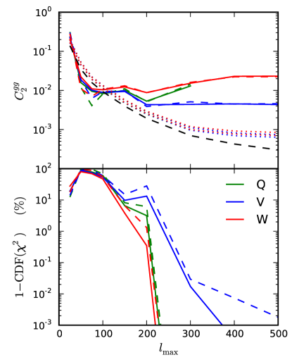
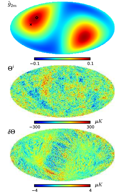
The $C_{l}$ of the QML quadrupole reconstructions are given in the top panel of Fig. 7 for the Q-, V- and W-band foreground-reduced datasets with a variety of cutoff $l_{\rm max}$ in the $l_{1},l_{2}$ sums of Eq. 26. In the lower panel are given the $\chi^{2}$ significances (calculated following Eq. 10), for a distribution with five degrees of freedom. At $l_{\rm max}\lesssim 150$ consistent results are seen in the Q-, V-, and W-band for all three datasets, independent of the choice of KQ75 or KQ85 masking, roughly tracing the amplitude of the estimator noise and consistent with no detection of anisotropy. Including data from higher multipoles, a highly significant excess power develops. The increasing discrepancy between the V- and W-band data at $l_{\rm max}>200$ seems indicative of systematic contamination rather than a primordial origin. To gain a better understanding of the required systematic, we use the algorithm described in Appendix A to generate a CMB realization which contains the observed modulation as the sum of anisotropic and purely isotropic parts. This is presented in the lower two panels of Fig. 8. The map of the anisotropic part gives a measure of the magnitude and spatial dependence of the systematic required to mimic the observed signal. The close alignment of the anomalous quadrupole modulation and the ecliptic seen in Fig. 8 suggests a systematic associated with the WMAP scan strategy. The two most suspicious possibilities are correlated noise and beam asymmetry effects, which have not been accounted for in this analysis, nor included in the Monte-Carlo simulations.

Ref. Groeneboom and Eriksen (2009) have already partially considered the effect of correlated noise on their results. Working with end-to-end simulations produced by the WMAP team for the 1-year data release, they find large effects for the W-band, although with qualitative structure different from that which is actually found in the data. In the quadratic-estimator approach, such possible contamination can be avoided by cross-correlating maps with different noise realizations, as discussed in Sec. II. Cross-correlating data for the individual differencing assemblies (D/As) of the V- and W-band data, we find that the anomalously large quadrupole power persists, further indicating that correlated noise is not a likely explanation for the observed excess.

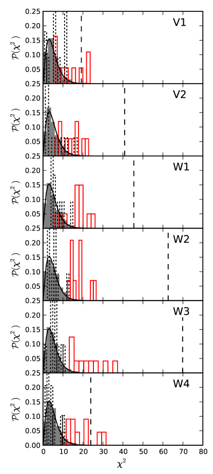
The effect of beam asymmetries is more involved, however a sample of the expected beam anisotropy effects can be found in Fig. 11 of Ref. Smith et al. (2007) and Fig. 5 of Wehus et al. (2009). The $1\mu\rm{K}$ RMS contribution of beam asymmetries to the observed sky is aligned with the ecliptic and matches well with the amplitude in our Fig. 8, making beam asymmetries a potential explanation for the observed anisotropy. To investigate this further, we analyze simulations of the WMAP data released by Ref. Wehus et al. (2009), who publish 10 maps of simulated beam-convolved skies for each of the WMAP D/As. The distribution of the resulting $\chi^{2}$ values is given in Fig. 9. The effect of asymmetric beams is seen to be large. For the V1 and W4 D/As, it completely explains the ${\cal O}(0.1\%)$ significance of the observed quadrupole. We therefore conclude that current measurements of the power modulation quadrupole are strongly contaminated by beam asymmetry effects, which must be corrected for to obtain true constraints on any primordial modulation. That the signal strongly varies between the D/As indicates either that the simulation of Ref. Wehus et al. (2009) are not encapsulating all of the relevant beam effects, or that there is an additional unknown systematic. In any case the significant variations between D/As at the same frequency provide strong evidence that the signal is systematic rather than primordial or foregrounds; in all cases the preferred direction is close to the ecliptic.

A full analysis with beam asymmetries is beyond the scope of this paper, however we note that in the QML approach beam asymmetry effects can simply be incorporated into the simulation pipeline. They will then appear as a contribution to the “mean field” term, and be subtracted from the reconstruction. In principle it is necessary to include the correlation due to beam asymmetries in the inverse variance filter, which is too computationally expensive to perform in general. If the instrumental noise can be approximated as white on the timescales which separate pixel visits, however, then the fast algorithm presented by Ref. Smith et al. (2007) can be used for the forward convolution operation, which should only slow the application of the inverse variance filter by a constant factor of ${\cal O}(20)$. Alternatively one could attempt to correct the maps for the beam asymmetries, for example by estimating the anisotropic contribution by forward convolutions of the observed sky, then iteratively subtracting off the part due to beam asymmetries.

Figure 9: Effect of beam asymmetry on the reconstruction of the $g(\hat{\mathbf{n}})$ quadrupole with $a(k)=1$, for the WMAP foreground-reduced data with KQ85 masking. Solid black is the $\chi^{2}$ distribution with five degrees of freedom. Gray histograms are the distribution of values for the isotropic simulations used to determine the estimator normalization for each D/A. Black vertical dashed lines indicate $\chi^{2}$ for the actual data. Red histograms are for the beam-convolved maps produced by Ref. Wehus et al. (2009). Black dotted histogram are for the input maps to the convolution, using symmetric beam transfer functions and separate noise realizations.

IV.3 Local primordial modulation

Figure 10: The $\alpha$ and $\beta$ functions for adiabatic transfer functions evaluated at $r_{*}=14164$Mpc, the comoving distance to the maximum visibility at the last scattering surface for our fiducial CMB parameters.

Finally, we consider the case where the primordial perturbations $\chi_{0}(\mathbf{x})$ are modulated in real space, so that the primordial perturbation field is

$$\chi(\mathbf{x})=\chi_{0}(\mathbf{x})[1+\phi(\mathbf{x})].$$ (28)

The primordial Gaussian field $\chi_{0}$ is assumed to be statistically homogeneous. Similar modulations have been considered before Dvorkin et al. (2008). We consider the modulating field $\phi(\mathbf{x})$ to be fixed, so the aim is to reconstruct the large-scale $\phi$ field by looking at the induced modulation of smaller-scale perturbations. To leading order in $\phi$ the primordial covariance is given by

$$\langle\chi(\mathbf{k})\chi(\mathbf{k}^{\prime})\rangle=(2\pi)^{3}\delta(\mathbf{k}+\mathbf{k}^{\prime})P_{\chi}(k)\\ +\int{\rm d}^{3}\mathbf{x}e^{-i(\mathbf{k}+\mathbf{k}^{\prime})\cdot\mathbf{x}}\phi(\mathbf{x})\left[P_{\chi}(k)+P_{\chi}(k^{\prime})\right].$$ (29)

Note that the modulated field (with fixed $\phi$) is no longer statistically homogeneous. Expanding the exponentials using

$$e^{i\mathbf{k}\cdot\mathbf{x}}=4\pi\sum_{lm}i^{l}j_{l}(kx)Y_{lm}(\hat{\mathbf{x}})Y_{lm}^{*}(\hat{\mathbf{k}}),$$ (30)

and using Eq. (19) to relate the primordial perturbations to the observed temperature multipoles, the covariance is then

$$C_{l_{1}m_{1}l_{2}m_{2}}=\delta_{l_{1}l_{2}}\delta_{m_{1}m_{2}}C_{l_{1}}$$

$$\quad+\int{\rm d}^{3}\mathbf{x}\phi(\mathbf{x})\alpha_{l_{1}}(x)\beta_{l_{2}}(x)Y_{l_{1}m_{1}}^{*}(\hat{\mathbf{x}})Y_{l_{2}m_{2}}(\hat{\mathbf{x}})$$

$$\quad+\int{\rm d}^{3}\mathbf{x}\phi(\mathbf{x})\alpha_{l_{2}}(x)\beta_{l_{1}}(x)Y_{l_{1}m_{1}}^{*}(\hat{\mathbf{x}})Y_{l_{2}m_{2}}(\hat{\mathbf{x}}),\quad$$ (31)

where

$$\alpha_{l}(r) \equiv 4\pi\int{\rm d}\ln kj_{l}(kr)\frac{k^{3}\Delta_{l}(k)}{2\pi^{2}}$$

$$\beta_{l}(r) \equiv 4\pi\int{\rm d}\ln kj_{l}(kr)\Delta_{l}(k)\mathcal{P}_{\chi}(k).$$ (32)

Hence using Eq (9) there is a QML estimator for the modulating field $\phi$ with

$$\tilde{h}^{\phi}_{lm}(r)=\int d\Omega Y_{lm}^{*}\left[\sum_{l_{1}m_{1}}\alpha_{l_{1}}(r)\bar{\Theta}_{l_{1}m_{1}}Y_{l_{1}m_{1}}\right]\\ \times\left[\sum_{l_{2}m_{2}}\beta_{l_{2}}(r)\bar{\Theta}_{l_{2}m_{2}}Y_{l_{2}m_{2}}\right].$$ (33)

This allows us to reconstruct a map of the modulation at any desired radius. The construction is very similar to that used when estimating a local bispectrum Komatsu et al. (2005); Smith and Zaldarriaga (2006), where the main quantity of interest is the correlation of the reconstructed $\phi$ with an estimator of $\chi$ (see Appendix B for further discussion). By looking at the modulating field directly, we can also consider the case where $\phi$ and $\chi$ are uncorrelated, and hence there is no leading-order bispectrum.

The isotropic component of the normalization is given by

$$\left[{\cal F}^{\phi\phi}_{\rm iso}\right]_{lm,l^{\prime}m^{\prime}}=\delta_{ll^{\prime}}\delta_{mm^{\prime}}\times\\ \sum_{l_{1},l_{2}}\frac{(2l_{1}+1)(2l_{2}+1)}{8\pi}{\begin{pmatrix}l&l_{1}&l_{2}\\ 0&0&0\end{pmatrix}}^{2}\frac{(\alpha_{l_{1}}\beta_{l_{2}}+\beta_{l_{1}}\alpha_{l_{2}})^{2}}{C^{\rm{tot}}_{l_{1}}C^{\rm{tot}}_{l_{2}}},$$ (34)

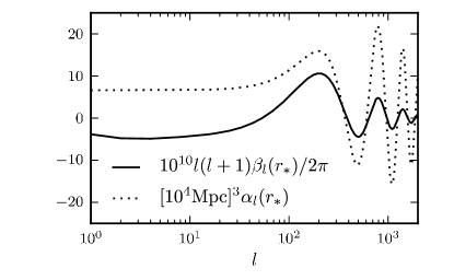
and typical $\alpha$ and $\beta$ functions are shown for adiabatic modes in Fig. 10.

Integrating $\tilde{h}^{\phi}_{lm}(r)$ over a window function $W(r)$ is equivalent to estimating a modulating field with that separable radial dependence; for large scale modulations with a constant $W(r)$ this is close to the spatial modulation estimator considered in Sec. IV.1 since any large-scale primordial modulation modulates essentially all of the CMB anisotropy sources in that direction (except possibly low redshift sources due to ISW that only effect low $l$). Mathematically this is because

$$\int r^{2}{\rm d}r\alpha_{l_{1}}(r)\beta_{l_{2}}(r)\sim C_{l_{1}}$$ (35)

for $l_{1}$ close to $l_{2}$ (with equality for $l_{1}=l_{2}$). We therefore do not repeat the analysis here, since the large-scale results of Sec. IV.1 with the full range of $l$ can be interpreted as being approximately a constraint on large-scale primordial modulations. We showed that any total modulation must be $\lesssim 1\%$ to be consistent the data on all scales, so modulation of primordial adiabatic modes would not explain the marginal evidence for a ${\cal O}(10\%)$ modulation at $l\lesssim 100$.

We can also consider the case where there is a modulated primordial isocurvature mode, combined with the usual unmodulated adiabatic mode. For example the modulation could be due to a large-scale perturbation in the background curvaton field Erickcek et al. (2009). The off-diagonal covariance in general depends on the power spectrum of the isocurvature modes as well as the correlation with the adiabatic modes, and the isotropic power spectrum is also modified due to the extra contributions (which gives a constraint on the amplitude of the isocurvature contributions). Estimators for the modulating field are of the same form as Eq. (32) but with the appropriate combinations of isocurvature transfer functions and power spectra: either $\alpha$ and $\beta$ both calculated with isocurvature transfer function, or the cross-estimator

$$\tilde{h}^{\phi_{ai}}_{lm}(r)=\frac{1}{2}\int d\Omega Y_{lm}^{*}\times\\ \biggl{(}\left[\sum_{l_{1}m_{1}}\alpha^{\text{Iso}}_{l_{1}}(r)\bar{\Theta}_{l_{1}m_{1}}Y_{l_{1}m_{1}}\right]\left[\sum_{l_{2}m_{2}}\beta_{l_{2}}^{\text{Ad}}(r)\bar{\Theta}_{l_{2}m_{2}}Y_{l_{2}m_{2}}\right]\\ +\left[\sum_{l_{1}m_{1}}\alpha^{\text{Ad}}_{l_{1}}(r)\bar{\Theta}_{l_{1}m_{1}}Y_{l_{1}m_{1}}\right]\left[\sum_{l_{2}m_{2}}\beta_{l_{2}}^{\text{Iso}}(r)\bar{\Theta}_{l_{2}m_{2}}Y_{l_{2}m_{2}}\right]\biggr{)}.$$ (36)

This corresponds to reconstructing the modulation of a primordial perturbation $\chi_{0}+\phi S$, where $S$ is taken to be a CDM isocurvature perturbation correlated to $\chi_{0}$. We assume the primordial adiabatic, isocurvature and cross power spectra are proportional, so up to normalization $\alpha$ and $\beta$ differ only in the transfer function used.

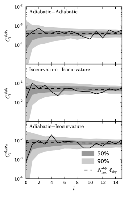
In Fig 11 we plot the pseudo-$C_{\ell}$ power spectrum of $\phi_{lm}$ reconstructed from the WMAP data for these models. Large scale modulations should be approximately constant across the depth of the last-scattering surface, and so we simply evaluate the estimator at the radius of peak visibility where most of the small-scale CMB fluctuations are coming from. The estimators at a given $r$ are significantly more noisy than the sky modulation estimators since the latter effectively average the result from many radial shells. We see no deviations from isotropy at the peak of the visibility.

Figure 11: Pseudo-$C_{l}$ of the $\phi_{lm}$ reconstructions for the WMAP V-band foreground-reduced data, with KQ85 mask and $l_{\rm max}=400$. The full-sky, isotropic normalization appropriate to each estimator was used rather than the actual inverse Fisher matrix. The $[25,75]\%$ (dark gray) and $[5,95]\%$ (light gray) confidence intervals measured from Monte-Carlo simulations are overlaid. The $\phi$ estimates are scaled by $\Delta_{r}[r^{*}]^{2}$ to give a dimensionless constraint, with $\Delta_{r}=100$Mpc, the approximate width of the last scattering surface.

As explained above, doing a constant line-of-sight integral is almost equivalent to a sky modulation for large-scale modulations. The same applies for isocurvature mode contributions (with greater accuracy since there is less contribution from ISW at low redshift), for example where the sky has adiabatic and isocurvature contributions:

$$\Theta(\hat{\mathbf{n}})=\Theta^{\text{Ad}}(\hat{\mathbf{n}})+\alpha[1+f(\hat{\mathbf{n}})]\Theta^{\text{Iso}}(\hat{\mathbf{n}}).$$ (37)

The isocurvature power spectrum $C^{\text{Iso}-\text{Iso}}_{l}$ falls off on sub-horizon scales, so the data is consistent with an ${\cal O}(10\%)$ dipole modulation of the total temperature if the modulation is only in the isocurvature component. The isotropic power spectrum constrains the isocurvature component to be subdominant however, so this would mean that an ${\cal O}(1)$ modulation of the isocurvature component is required, which would invalidate the assumptions in deriving the sky modulation estimator that $|f|\ll 1$. However we can still apply a null-hypothesis test on a purely isotropic adiabatic model using whatever parameterization we like, though interpretation of any detection of deviation may need to be treated with care. We do not attempt a fully consistent analysis of isotropic and anisotropic constraints on isocurvature contributions here.

The isocurvature mode could also be correlated with the adiabatic mode, in which case we can constrain a model of the form

$$\Theta(\hat{\mathbf{n}})=\Theta^{\text{Ad}}(\hat{\mathbf{n}})+f(\hat{\mathbf{n}})\Theta^{\text{Iso}}(\hat{\mathbf{n}}),$$ (38)

where $\langle\Theta_{lm}^{\text{Ad}}\Theta^{\text{Iso}*}_{lm}{}\rangle=\alpha C^{\text{Ad}-\text{Iso}}_{l}$, $\alpha$ depends on the amplitude and degree of correlation, and $C^{\text{Ad}-\text{Iso}}_{l}$ is the spectrum for totally correlated modes with the same initial amplitude ($S=-\chi_{0}$). As usual we neglect terms of ${\cal O}(f^{2})$. The monopole part of $f$ allows for an isotropic isocurvature contribution. The estimators are almost the same as in the total temperature modulation case, with

$$\tilde{h}^{f}_{lm}=\int d\Omega Y_{lm}^{*}\left[\sum_{l_{1}m_{1}}^{l_{\rm max}}\bar{\Theta}_{l_{1}m_{1}}Y_{l_{1}m_{1}}\right]\left[\sum_{l_{2}m_{2}}^{l_{\rm max}}C^{X}_{l_{2}}\bar{\Theta}_{l_{2}m_{2}}Y_{l_{2}m_{2}}\right],$$ (39)

where $C^{X}_{l}$ is the relevant power spectrum, and we evaluate $\bar{\Theta}_{lm}$ using the standard best-fit theory model in the assumption that a model with isocurvature modes must have about the same spectrum as the null hypothesis with no isocurvature modes. A more general model could also allow part of the adiabatic mode to be modulated.

The constraint on isocurvature modulations is shown in Fig. 12, though the data is still consistent with isotropy at the $1\%$-level. See Ref. Erickcek et al. (2009) for more detailed discussion and possible physical mechanisms for generating modulated isocurvature modes.

Figure 12: Same as Fig. 3 but using the power spectra for the indicated combinations of adiabatic and isocurvature transfer functions in the estimator (replacing $C_{l_{2}}$ in Eq. (17)). All curves are for the WMAP V-band foreground-reduced data with KQ85 masking.

We have focussed on local modulations here, however the formalism can in principle be applied to more general primordial anisotropic models, for instance with

$$\chi(\mathbf{x})=\chi_{0}(\mathbf{x})+\\ \int\frac{{\rm d}^{3}\mathbf{k}_{1}}{(2\pi)^{3}}\frac{{\rm d}^{3}\mathbf{k}_{2}}{(2\pi)^{3}}f(\mathbf{k}_{1},\mathbf{k}_{2})\chi_{0}(\mathbf{k}_{1})\phi(\mathbf{k}_{2})e^{i(\mathbf{k}_{1}+\mathbf{k}_{2})\cdot\mathbf{x}}.$$ (40)

Such more general forms can arise for example in warm inflation Moss and Xiong (2007) and other models giving non-local primordial bispectrum non-Gaussianity (see e.g. Ref. Fergusson and Shellard (2008)). A detailed analysis is beyond the scope of this paper, but is similar to that required to constrain the bispectrum when $\phi$ is equal to $\chi_{0}$.

V Conclusions

The assumption that the CMB is statistically isotropic is a common one in modern cosmology, and needs to be rigorously tested. In this paper, we argued that QML estimators are often ideal for this purpose. They provide optimal, minimum-variance constraints and permit straightforward systematic and jacknife tests. We have demonstrated their use in application to the WMAP dataset for constraining several anisotropic models. Most notably, we reproduced the results of previous exact likelihood analyses which showed marginal evidence for a dipolar modulation of the observed CMB for $l<100$. However we showed that the amplitude of the modulation must fall significantly on smaller scales, consistent with observations that the small scale power in the universe (e.g. probed by quasars Hirata (2009)) appears to be highly isotropic. This scale-dependence is inconsistent with modulated adiabatic primordial modes, but could possibly be explained by modulated isocurvature modes, which have less power on small scales. However evidence for deviations from isotropy are only at the $1\%$-level.

We also studied a model in which the primordial power spectrum has a direction dependence, detecting a significant anisotropy in the WMAP maps with close-to-ecliptic alignment. However we argued that this signal has an important contribution from beam asymmetries, which are uncorrected in the maps, and that significant variations between differencing assemblies indicate that most of the signal is non-primordial.

An important extension of this approach is the inclusion of polarization data. For anisotropies which are detected in temperature at marginal significance, polarization can help to increase the signal to noise and to distinguish possible primordial, local and systematic origins of any detection Dvorkin et al. (2008).

VI Acknowledgements

AL acknowledges a PPARC/STFC advanced fellowship and thanks the Aspen Center for Physics for hospitality while part of this work in progress, and workshop participants for useful discussions. DH is grateful for the support of a Gates scholarship. We thank Anthony Challinor for helpful suggestions and Hiranya Peiris, Andrew Pontzen, Kendrick Smith and Douglas Scott for numerous related discussions. Some of the results in this paper have been derived using HEALPix Gorski et al. (2005). We acknowledge the use of the Legacy Archive for Microwave Background Data Analysis (LAMBDA). Support for LAMBDA is provided by the NASA Office of Space Science.

Appendix A Anisotropic Simulations

Here we present an algorithm for generating weakly anisotropic simulations. We wish to sample from a Gaussian distribution with covariance

$$\bm{C}=(\bm{I}+\delta\bm{C}[\bm{C}^{i}]^{-1})\bm{C}^{i}$$ (41)

where $\bm{C}^{i}$ is isotropic and $\delta\bm{C}$ is the small anisotropic part. Then

$$\mathbf{\Theta}=\left[\bm{I}+\delta\bm{C}[\bm{C}^{i}]^{-1}\right]^{1/2}\mathbf{\Theta}^{i},$$ (42)

where $\mathbf{\Theta}^{i}$ has covariance $\bm{C}^{i}$ will have the required covariance. For small anisotropy this can be expanded to give

$$\mathbf{\Theta}\approx\mathbf{\Theta}^{i}+\frac{1}{2}\delta\bm{C}[\bm{C}^{i}]^{-1}\mathbf{\Theta}^{i}+\dots.$$ (43)

Higher order terms can be included if required; here we just calculate the leading anisotropic term. In the case of an anisotropic primordial power spectrum this is

$$\delta\mathbf{\Theta}_{lm}\approx\frac{1}{2}\int{\rm d}\Omega Y_{lm}^{*}g\left[\sum_{l_{2}m_{2}}i^{l-l_{2}}\frac{C_{ll_{2}}\Theta^{i}_{l_{2}m_{2}}}{C_{l_{2}}}Y_{l_{2}m_{2}}\right].$$ (44)

Appendix B Relation to bispectrum estimators

Power anisotropy is closely related to primordial non-Gaussianity. Local non-Gaussianity gives power in squeezed triangles: large scale perturbations are correlated to small scale power over their extent. If the large scale perturbation were unknown, this would look just like a small-scale power anisotropy. Hence a method that reconstructs the power anisotropy should be sensitive to three-point non-Gaussianity, in that the correlation of the anisotropy estimator with the temperature is a probe of the bispectrum. Non-Gaussianity can also give rise to a dipole power asymmetry correlated with the (unknown) cosmological dipole. In the inflationary context a power anisotropy on a given scale typically indicates the impact of those modes when they were outside the horizon on the generation of smaller fluctuations, e.g. via the local change in the effective background seen by the smaller modes as they leave the horizon. Unfortunately the large variance of the anisotropy estimators means that for small amounts of non-Gaussianity any detection with standard shapes is expected to be via the correlation to the temperature, as in standard bispectrum analyses. However since there is marginal evidence for power anisotropies in the data it is worth considering whether these could be associated with some form of physically-motivated primordial non-Gaussianity. There may also be marginal observational evidence for local primordial bispectrum non-Gaussianity Yadav and Wandelt (2008); Komatsu et al. (2009); Smith et al. (2009), so conceivably there could be a joint explanation.

A statistically-isotropic and parity-invariant CMB bispectrum $B_{l_{1}l_{2}l_{3}}$ is defined by

$$\langle a_{l_{1}m_{1}}a_{l_{2}m_{2}}a_{l_{3}m_{3}}\rangle \equiv B_{l_{1}l_{2}l_{3}}{\begin{pmatrix}l_{1}&l_{2}&l_{3}\\ m_{1}&m_{2}&m_{3}\end{pmatrix}}$$ (45)

$$= b_{l_{1}l_{2}l_{3}}\int{\rm d}\Omega Y_{l_{1}m_{1}}Y_{l_{2}m_{2}}Y_{l_{3}m_{3}},\qquad$$ (46)

where $b_{l_{1}l_{2}l_{3}}$ is the reduced bispectrum. When the CMB power spectrum is known, the optimal estimator for weakly non-Gaussian fields with bispectrum $B_{l_{1}l_{2}l_{3}}$ is Creminelli et al. (2006); Babich (2005); Smith and Zaldarriaga (2006)

$$\mathcal{E}=N_{\mathcal{E}}^{-1}\sum_{l_{i}m_{i}}B_{l_{1}l_{2}l_{3}}{\begin{pmatrix}l_{1}&l_{2}&l_{3}\\ m_{1}&m_{2}&m_{3}\end{pmatrix}}\\ \times\biggl{[}\bar{\Theta}_{l_{1}m_{1}}\bar{\Theta}_{l_{2}m_{2}}\bar{\Theta}_{l_{3}m_{3}}-3C^{-1}_{l_{1}m_{1}l_{2}m_{2}}\bar{\Theta}_{l_{3}m_{3}}\biggr{]},$$ (47)

where $N_{\mathcal{E}}$ is a normalization. Following Ref. Smith and Zaldarriaga (2006) this can be written as

$$\mathcal{E}=\frac{1}{N_{\mathcal{E}}}\sum_{lm}\bar{\Theta}_{lm}^{*}(X_{lm}-3\langle X_{lm}\rangle)$$ (48)

where

$$X_{lm} = \sum_{l_{1}m_{1},l_{2}m_{2}}B_{ll_{1}l_{2}}(-1)^{m_{1}}{\begin{pmatrix}l&l_{1}&l_{2}\\ m&-m_{1}&m_{2}\end{pmatrix}}\bar{\Theta}_{l_{1}m_{1}}\bar{\Theta}_{l_{2}m_{2}}^{*}$$ (49)

$$= \int{\rm d}\Omega Y_{lm}^{*}\times$$

$$\sum_{l_{1}l_{2}}b_{ll_{1}l_{2}}\left[\sum_{m_{1}}\bar{\Theta}_{l_{1}m_{1}}Y_{l_{1}m_{1}}\right]\left[\sum_{m_{2}}\bar{\Theta}_{l_{2}m_{2}}Y_{l_{2}m_{2}}\right].$$

The $X_{lm}$ field is of the form of the most general quadratic anisotropy estimator, with free weighting coefficients $b_{ll_{1}l_{2}}$. Bispectrum estimators are essentially correlations of specific power anisotropy estimators with the temperature.

Often the dipole $\Theta_{1m}$ is projected out of bispectrum analyses, effectively ignoring $X_{1m}$, even though in general $X_{lm}$ contains interesting power asymmetry information that could be generated by non-Gaussianity. The ‘optimal’ bispectrum estimator is only optimal with certain assumptions; if the temperature dipole information is removed then the dipole part of the power anisotropy should contain additional information about the non-Gaussianity, which in principle could improve constraints if the non-Gaussianity is larger than the anisotropy expected from lensing and doppler effects. This is equivalent to using part of the trispectrum, see Refs. Kogo and Komatsu (2006); Creminelli et al. (2007) for further discussion.

A primordial statistically isotropic bispectrum can be defined as

$$\langle\chi_{0}(\mathbf{k}_{1})\chi_{0}(\mathbf{k}_{2})\chi_{0}(\mathbf{k}_{3})\rangle=(2\pi)^{3}\delta(\mathbf{k}_{1}+\mathbf{k}_{2}+\mathbf{k}_{3})B_{\chi}(k_{1},k_{2},k_{3}).$$ (50)

For local non-Gaussianity

$$B_{\chi}(k_{1},k_{2},k_{3})=\pm 2\frac{3}{5}f_{NL}(P_{\chi}(k_{1})P_{\chi}(k_{2})+\text{2 perms.})$$ (51)

where the $3/5$ is conventional (from relation the curvature perturbation to the Newtonian potential in the radiation dominated era) and $\pm$ is a sign convention. The reduced bispectrum is then

$$b_{l_{1}l_{2}l_{3}}=\pm\frac{3}{5}f_{NL}\int r^{2}{\rm d}r\beta_{l_{1}}(r)\beta_{l_{2}}(r)\alpha_{l_{3}}(r)+\text{5 perms.}$$ (52)

We can relate this to our local spatial modulation estimator of Eq. 33 by windowing to give a line-of-sight average of the primordial modulating field

$$\bar{h}_{lm}=\int{\rm d}rr^{2}\tilde{h}_{lm}^{\phi}(r)W_{l}(r)=\int{\rm d}\Omega Y_{lm}^{*}\\ \times\sum_{l_{1}l_{2}}b_{ll_{1}l_{2}}\left[\sum_{m_{1}}\bar{\Theta}_{l_{1}m_{1}}Y_{l_{1}m_{1}}\right]\left[\sum_{m_{2}}\bar{\Theta}_{l_{2}m_{2}}Y_{l_{2}m_{2}}\right].$$ (53)

This is of the form of a general quadratic anisotropy estimator, but with weights in the specific form

$$b_{ll_{1}l_{2}}=\int{\rm d}rr^{2}W_{l}(r)\alpha_{l_{1}}(r)\beta_{l_{2}}(r).$$ (54)

If the modulating field is the primordial field itself, $\phi=\chi_{0}$, there is local bispectrum. In this case choosing $W_{l}(r)=\beta_{l}(r)$ relates the primordial field to the observed temperature, since $\beta(r)\bar{\Theta}_{lm}$ is the minimum variance estimate for the primordial field at $r$ Komatsu et al. (2005). Then $b_{ll_{1}l_{2}}$ is the form of the reduced bispectrum obtained by correlating $\bar{h}_{lm}$ with the temperature $\bar{\Theta}_{lm}$.

References

- Tegmark et al. (2003) M. Tegmark, A. de Oliveira-Costa, and A. Hamilton, Phys. Rev. D68, 123523 (2003), astro-ph/0302496.
- Bielewicz et al. (2004) P. Bielewicz, K. M. Gorski, and A. J. Banday, Mon. Not. Roy. Astron. Soc. 355, 1283 (2004), astro-ph/0405007.
- Copi et al. (2006) C. J. Copi, D. Huterer, D. J. Schwarz, and G. D. Starkman, Mon. Not. Roy. Astron. Soc. 367, 79 (2006), astro-ph/0508047.
- Land and Magueijo (2005) K. Land and J. Magueijo, Phys. Rev. Lett. 95, 071301 (2005), astro-ph/0502237.
- Hansen et al. (2008) F. K. Hansen, A. J. Banday, K. M. Gorski, H. K. Eriksen, and P. B. Lilje (2008), 0812.3795.
- Eriksen et al. (2004) H. K. Eriksen, F. K. Hansen, A. J. Banday, K. M. Gorski, and P. B. Lilje, Astrophys. J. 605, 14 (2004), astro-ph/0307507.
- Cruz et al. (2007) M. Cruz, L. Cayon, E. Martinez-Gonzalez, P. Vielva, and J. Jin, Astrophys. J. 655, 11 (2007), astro-ph/0603859.
- Lewis and Challinor (2006) A. Lewis and A. Challinor, Phys. Rept. 429, 1 (2006), astro-ph/0601594.
- Dvorkin and Smith (2009) C. Dvorkin and K. M. Smith, Phys. Rev. D79, 043003 (2009), 0812.1566.
- Gumrukcuoglu et al. (2007) A. E. Gumrukcuoglu, C. R. Contaldi, and M. Peloso, JCAP 0711, 005 (2007), 0707.4179.
- Ackerman et al. (2007) L. Ackerman, S. M. Carroll, and M. B. Wise, Phys. Rev. D75, 083502 (2007), astro-ph/0701357.
- Bond et al. (2009) J. R. Bond, A. V. Frolov, Z. Huang, and L. Kofman, Phys. Rev. Lett. 103, 071301 (2009), 0903.3407.
- Chang et al. (2009) S. Chang, M. Kleban, and T. S. Levi, JCAP 0904, 025 (2009), 0810.5128.
- Cruz et al. (2008) M. Cruz et al. (2008), 0804.2904.
- Gordon (2007) C. Gordon, Astrophys. J. 656, 636 (2007), astro-ph/0607423.
- Hoftuft et al. (2009) J. Hoftuft et al. (2009), 0903.1229.
- Groeneboom and Eriksen (2009) N. E. Groeneboom and H. K. Eriksen, Astrophys. J. 690, 1807 (2009), 0807.2242.
- Hirata and Seljak (2003) C. M. Hirata and U. Seljak, Phys. Rev. D67, 043001 (2003), astro-ph/0209489.
- Dvorkin et al. (2008) C. Dvorkin, H. V. Peiris, and W. Hu, Phys. Rev. D77, 063008 (2008), 0711.2321.
- Pullen and Kamionkowski (2007) A. R. Pullen and M. Kamionkowski, Phys. Rev. D76, 103529 (2007), 0709.1144.
- Armendariz-Picon (2006) C. Armendariz-Picon, JCAP 0603, 002 (2006), astro-ph/0509893.
- Prunet et al. (2005) S. Prunet, J.-P. Uzan, F. Bernardeau, and T. Brunier, Phys. Rev. D71, 083508 (2005), astro-ph/0406364.
- Tegmark (1997) M. Tegmark, Phys. Rev. D55, 5895 (1997), astro-ph/9611174.
- Okamoto and Hu (2003) T. Okamoto and W. Hu, Phys. Rev. D67, 083002 (2003), astro-ph/0301031.
- Hinshaw et al. (2009) G. Hinshaw et al. (WMAP), Astrophys. J. Suppl. 180, 225 (2009), 0803.0732.
- Oh et al. (1999) S. P. Oh, D. N. Spergel, and G. Hinshaw, Astrophys. J. 510, 551 (1999), astro-ph/9805339.
- Dunkley et al. (2009) J. Dunkley et al. (WMAP), Astrophys. J. Suppl. 180, 306 (2009), 0803.0586.
- Smith et al. (2007) K. M. Smith, O. Zahn, and O. Dore, Phys. Rev. D76, 043510 (2007), 0705.3980.
- Gordon et al. (2005) C. Gordon, W. Hu, D. Huterer, and T. Crawford, Phys. Rev. D 72, 103002 (2005), .
- Hansen et al. (2004) F. K. Hansen, A. J. Banday, and K. M. Gorski, Mon. Not. Roy. Astron. Soc. 354, 641 (2004), astro-ph/0404206.
- Spergel et al. (2006) D. N. Spergel et al. (2006), astro-ph/0603449v1.
- Eriksen et al. (2007) H. K. Eriksen, A. J. Banday, K. M. Gorski, F. K. Hansen, and P. B. Lilje, Astrophys. J. 660, L81 (2007), astro-ph/0701089.
- Challinor and Sollom (2009) A. Challinor and I. Sollom, In prep. (2009).
- Hajian and Souradeep (2003) A. Hajian and T. Souradeep, Astrophys. J. 597, L5 (2003), astro-ph/0308001.
- Cruz et al. (2005) M. Cruz, E. Martinez-Gonzalez, P. Vielva, and L. Cayon, Mon. Not. Roy. Astron. Soc. 356, 29 (2005), astro-ph/0405341.
- Hirata (2009) C. M. Hirata (2009), 0907.0703.
- Gold et al. (2009) B. Gold et al. (WMAP), Astrophys. J. Suppl. 180, 265 (2009), 0803.0715.
- Yokoyama and Soda (2008) S. Yokoyama and J. Soda, JCAP 0808, 005 (2008), 0805.4265.
- Dimopoulos et al. (2009) K. Dimopoulos, M. Karciauskas, D. H. Lyth, and Y. Rodriguez, JCAP 0905, 013 (2009), 0809.1055.
- Smith and Zaldarriaga (2006) K. M. Smith and M. Zaldarriaga (2006), astro-ph/0612571.
- Wehus et al. (2009) I. K. Wehus, L. Ackerman, H. K. Eriksen, and N. E. Groeneboom, Astrophys. J. 707, 343 (2009), 0904.3998.
- Komatsu et al. (2005) E. Komatsu, D. N. Spergel, and B. D. Wandelt, Astrophys. J. 634, 14 (2005), astro-ph/0305189.
- Erickcek et al. (2009) A. L. Erickcek, C. M. Hirata, and M. Kamionkowski, Phys. Rev. D80, 083507 (2009), 0907.0705.
- Moss and Xiong (2007) I. G. Moss and C. Xiong, JCAP 0704, 007 (2007), astro-ph/0701302.
- Fergusson and Shellard (2008) J. R. Fergusson and E. P. S. Shellard (2008), 0812.3413.
- Gorski et al. (2005) K. M. Gorski et al., Astrophys. J. 622, 759 (2005), astro-ph/0409513.
- Yadav and Wandelt (2008) A. P. S. Yadav and B. D. Wandelt, Phys. Rev. Lett. 100, 181301 (2008), 0712.1148.
- Komatsu et al. (2009) E. Komatsu et al. (WMAP), Astrophys. J. Suppl. 180, 330 (2009), 0803.0547.
- Smith et al. (2009) K. M. Smith, L. Senatore, and M. Zaldarriaga (2009), 0901.2572.
- Creminelli et al. (2006) P. Creminelli, A. Nicolis, L. Senatore, M. Tegmark, and M. Zaldarriaga, JCAP 0605, 004 (2006), astro-ph/0509029.
- Babich (2005) D. Babich, Phys. Rev. D72, 043003 (2005), astro-ph/0503375.
- Kogo and Komatsu (2006) N. Kogo and E. Komatsu, Phys. Rev. D73, 083007 (2006), astro-ph/0602099.
- Creminelli et al. (2007) P. Creminelli, L. Senatore, and M. Zaldarriaga, JCAP 0703, 019 (2007), astro-ph/0606001.