Solitons, peakons and periodic cusp wave solutions for the Fornberg-Whitham equation

Abstract

In this paper, we employ the bifurcation method of dynamical systems to investigate the exact travelling wave solutions for the Fornberg-Whitham equation $u_{t}-u_{xxt}+u_{x}+uu_{x}=uu_{xxx}+3u_{x}u_{xx}$. The implicit expression for solitons is given. The explicit expressions for peakons and periodic cusp wave solutions are also obtained. Further, we show that the limits of soliton solutions and periodic cusp wave solutions are peakons.

,

1 Introduction

The Fornberg-Whitham equation

$$u_{t}-u_{xxt}+u_{x}+uu_{x}=uu_{xxx}+3u_{x}u_{xx},$$ (1.1)

has appeared in the study of qualitative behaviors of wave breaking [1, 2]. It is a nonlinear dispersive wave equation. Since Eq.(1.1) was derived, little attention has been paid to studying it. In [3], Fornberg and Whitham obtained a peaked solution of the form $u(x,t)=A\exp{(-\frac{1}{2}\left|{x-\frac{4}{3}t}\right|)}$, where $A$ is an arbitrary constant. In [4], we constructed a type of bounded travelling wave solutions for Eq.(1.1), which are called kink-like and antikink-like wave solutions. Unfortunately, the results in [3, 4] are not complete. In the present paper, we continue to derive more travelling wave solutions for Eq.(1.1), so that we can supplement the results of [3, 4].

The remainder of the paper is organized as follows. In Section 2, we discuss the bifurcation curves and phase portraits of travelling wave system. In Section 3, we obtain the implicit expression for solitons and the explicit expressions for peakons and periodic cusp wave solutions. At the same time, we show that the limits of solitons and periodic cusp wave solutions are peakons. A short conclusion is given in Section 4.

2 Bifurcation and phase portraits of travelling wave system

Let $u=\varphi(\xi)$ with $\xi=x-ct$ be the solution for Eq.(1.1); then it follows that

$$-c\varphi^{\prime}+c\varphi^{\prime\prime\prime}+\varphi^{\prime}+\varphi\varphi^{\prime}=\varphi\varphi^{\prime\prime\prime}+3\varphi^{\prime}\varphi^{\prime\prime}.$$ (2.1)

Integrating Eq. (2.1) once we have

$$\varphi^{\prime\prime}(\varphi-c)=g-c\varphi+\varphi+\frac{1}{2}\varphi^{2}-(\varphi^{\prime})^{2},$$ (2.2)

where $g$ is the integral constant.

Let $y=\varphi^{\prime}$; then we get the following planar dynamical system:

$$\left\{{\begin{array}[]{l}\frac{\textstyle d\varphi}{\textstyle d\xi}=y,\\ \frac{\textstyle dy}{\textstyle d\xi}=\frac{\textstyle g-c\varphi+\varphi+\frac{1}{2}\varphi^{2}-y^{2}}{\textstyle\varphi-c},\end{array}}\right.$$ (2.3)

with a first integral

$$H(\varphi,y)=(\varphi-c)^{2}(y^{2}-\frac{1}{4}\varphi^{2}+(\frac{1}{2}c-\frac{2}{3})\varphi+\frac{1}{4}c^{2}-\frac{1}{3}c-g)=h,$$ (2.4)

where $h$ is a constant.

Note that (2.3) has a singular line $\varphi=c$. To avoid the line temporarily we make transformation $d\xi=(\varphi-c)d\zeta$. Under this transformation, Eq.(2.3) becomes

$$\left\{{\begin{array}[]{l}\frac{\textstyle d\varphi}{\textstyle d\zeta}=(\varphi-c)y,\\ \frac{\textstyle dy}{\textstyle d\zeta}=g-c\varphi+\varphi+\frac{1}{2}\varphi^{2}-y^{2}.\\ \end{array}}\right.$$ (2.5)

System (2.3) and system (2.5) have the same first integral as (2.4). Consequently, system (2.5) has the same topological phase portraits as system (2.3) except for the straight line $\varphi=c$. Obviously, $\varphi=c$ is an invariant straight-line solution for system (2.5).

For a fixed $h$, (2.4) determines a set of invariant curves of system (2.5). As $h$ is varied, (2.4) determines different families of orbits of system (2.5) having different dynamical behaviors. Let $M(\varphi_{e},y_{e})$ be the coefficient matrix of the linearized version of (2.5) at the equilibrium point $(\varphi_{e},y_{e})$; then

$$M(\varphi_{e},y_{e})=\left({{\begin{array}[]{*{20}c}{\quad\quad y_{e}\hfill}&&&{\varphi_{e}-c\hfill}\\ {\varphi_{e}-(c-1)\hfill}&&&{-2y_{e}\hfill}\\ \end{array}}}\right)$$ (2.6)

and at this equilibrium point, we have

$$J(\varphi_{e},y_{e})=\det M(\varphi_{e},y_{e})=-2y_{e}^{2}-(\varphi_{e}-c)[\varphi_{e}-(c-1)],$$ (2.7)

$$p(\varphi_{e},y_{e})=\mathrm{trace}(M(\varphi_{e},y_{e}))=-y_{e}.$$ (2.8)

By the theory of planar dynamical systems (see [5]), for an equilibrium point of a planar dynamical system, if $J<0$, then this equilibrium point is a saddle point; it is a center point if $J>0$ and $p=0$; if $J=0$ and the Poincaré index of the equilibrium point is 0, then it is a cusp.

By using the first-integral value and properties of equilibrium points, we obtain the bifurcation curves as follows:

$$g_{1}(c)=\frac{1}{2}(c-1)^{2},$$ (2.9)

$$g_{2}(c)=\frac{1}{2}(c-1)^{2}-\frac{1}{18},$$ (2.10)

$$g_{3}(c)=\frac{1}{2}(c-1)^{2}-\frac{1}{2}.$$ (2.11)

Obviously, the three curves have no intersection point and $g_{3}(c)<g_{2}(c)<g_{1}(c)$ for arbitrary constant $c$.

Using the bifurcation method for vector fields (e.g., [5]), we have the following result which describes the locations and properties of the singular points of system (2.5).

Theorem 2.1

For given any constant wave speed $c\neq 0$, let

$$\varphi_{1\pm}=c-1\pm\sqrt{(c-1)^{2}-2g}\quad for\quad g\leq g_{1}(c),$$ (2.12)

$$y_{1\pm}=\pm\sqrt{g-\frac{1}{2}c^{2}+c}\quad for\quad g\geq g_{3}(c).$$ (2.13)

Then we have

(1)If $g<g_{3}(c)$, then system (2.5) has two equilibrium points $(\varphi_{1-},0)$ and $(\varphi_{1+},0)$, which are saddle points.

(2)If $g=g_{3}(c)$, then system (2.5) has two equilibrium points $(c-2,0)$ and $(c,0)$. $(c-2,0)$ is a saddle point and $(c,0)$ is a cusp.

(3)If $g_{3}(c)<g<g_{2}(c)$, then system (2.5) has four equilibrium points $(\varphi_{1-},0)$, $(\varphi_{1+},0)$, $(c,y_{1-})$ and $(c,y_{1+})$. $(\varphi_{1-},0)$ is a saddle point and $(\varphi_{1+},0)$ is a center point enclosing the orbit which connects the saddle points $(c,y_{1-})$ and $(c,y_{1+})$.

(4)If $g=g_{2}(c)$, then system (2.5) has four equilibrium points $(c-\frac{4}{3},0)$, $(c-\frac{2}{3},0)$, $(c,-\frac{2}{3})$ and $(c,\frac{2}{3})$, which satisfy $H(c-\frac{4}{3},0)=H(c,-\frac{2}{3})=H(c,\frac{2}{3})$ and form a triangular orbit which encloses the center point $(c-\frac{2}{3},0)$.

(5)If $g_{2}(c)<g<g_{1}(c)$, then system (2.5) has four equilibrium points $(\varphi_{1-},0)$, $(\varphi_{1+},0)$, $(c,y_{1-})$ and $(c,y_{1+})$. $(\varphi_{1+},0)$ is a center point enclosing the orbit which is homoclinic for the saddle point $(\varphi_{1-},0)$.

(6)If $g=g_{1}(c)$, then system (2.5) has three equilibrium points $(c-1,0)$, $(c,-\frac{\sqrt{2}}{2})$ and $(c,\frac{\sqrt{2}}{2})$. $(c-1,0)$ is a cusp. $(c,-\frac{\sqrt{2}}{2})$ and $(c,\frac{\sqrt{2}}{2})$ are two saddle points.

(7)If $g>g_{1}(c)$, then system (2.5) has two equilibrium points $(c,y_{1-})$ and $(c,y_{1+})$. They are saddle points.

The phase portraits of system (2.5) are given in Fig.1.

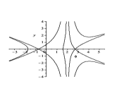
(a)

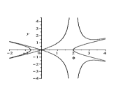
(b)

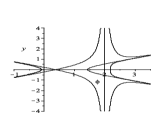
(c)

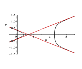
(d)

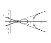
(e)

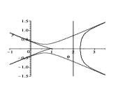
(f)

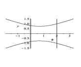
(g)

Figure 1: The phase portraits of system (2.5). (a) $g<g_{3}(c)$; (b) $g=g_{3}(c)$; (c) $g_{3}(c)<g<g_{2}(c)$; (d) $g=g_{2}(c)$; (e) $g_{2}(c)<g<g_{1}(c)$; (f) $g=g_{1}(c)$; (g) $g>g_{1}(c)$.

3 Solitons, peakons and periodic cusp wave solutions

Suppose that $\varphi(\xi)(\xi=x-ct)$ is a travelling wave solution for Eq.(1.1) for $\xi\in(-\infty,+\infty)$, and $\mathop{\lim}\limits_{\xi\to-\infty}\varphi(\xi)=A$, $\mathop{\lim}\limits_{\xi\to\infty}\varphi(\xi)=B$, where $A$ and $B$ are two constants. If $A=B$, then $\varphi(\xi)$ is called a soliton solution. If $A\neq B$, then $\varphi(\xi)$ is called a kink (or an antikink) solution. Usually, a soliton solution for Eq.(1.1) corresponds to a homoclinic orbit of system (2.3) and a periodic travelling wave solution for Eq.(1.1) corresponds to a periodic orbit of system (2.3). Similarly, a kink (or an antikink) wave solution of Eq.(1.1) corresponds to a heteroclinic orbit (or the so-called connecting orbit) of system (2.3). The graphs of the homoclinic orbit, periodic orbit and their limit cure are shown in Fig.2.

The following lemma gives the relationship of soliton solutions of Eq.(1.1) and homoclinic orbits of system (2.3).

Lemma 3.1

Assume that $\Gamma$ is a homoclinic orbit of system (2.3) and its parameter expression is $\varphi=\varphi(\xi)$ and $y=y(\xi)$; then $u=\varphi(\xi)$ with $\xi=x-ct$ is a soliton solution for Eq.(1.1).

Proof. From Fig.1(e), we can see that the homoclinic orbit $\Gamma$ encloses $(\varphi_{1+},0)$ and connects $(\varphi_{1-},0)$. Therefore, $\lim_{|\xi|\rightarrow\infty}\varphi(\xi)=\varphi_{1-}$.

On the other hand, $u=\varphi(\xi)$ is the solution for system (2.3). This implies that $u=\varphi(\xi)$ is the solution for Eq.(2.1). Thus, $u=\varphi(x-ct)$ is the soliton solution for Eq.(1.1).  

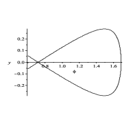
(a)

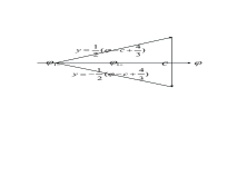
(b)

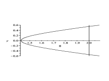
(c)

Figure 2: The orbits of system (2.3). (a) The homoclinic orbit (corresponding to $g_{2}(c)<g<g_{1}(c)$). (b) The limit curve of homoclinic orbit and periodic orbit (corresponding to $g=g_{2}(c)$). (c) The periodic orbit (corresponding to $g_{3}(c)<g<g_{2}(c)$).

In Fig.2(a), the homoclinic orbit of system (2.3) can be expressed as

$$y=\pm\frac{(\varphi-\varphi_{1-})\sqrt{\varphi^{2}+l_{1}\varphi+l_{2}}}{2(\varphi-c)}\quad for\quad\varphi_{1-}<\varphi<\varphi_{2+},$$ (3.1)

where

$$l_{1}=\frac{2}{3}(1-3c-3\sqrt{(c-1)^{2}-2g}),$$ (3.2)

$$l_{2}=\frac{2}{3}(1-4c+3c^{2}-3g+(3c+1)\sqrt{(c-1)^{2}-2g}),$$ (3.3)

$$\varphi_{2+}=-\frac{1}{3}(1-3c-3\sqrt{(c-1)^{2}-2g}+2\sqrt{1-3\sqrt{(c-1)^{2}-2g}}).$$ (3.4)

Substituting Eq.(3.1) into the first equation of system (2.3) and integrating along the homoclinic orbits, we have

$${\int_{\varphi}^{\varphi_{2+}}{\frac{s-c}{(s-\varphi_{1-})\sqrt{s^{2}+l_{1}s+l_{2}}}ds=-\frac{1}{2}|\xi|}}.$$ (3.5)

It follows from (3.5) that

$$\beta(\varphi_{2+})=\beta(\varphi)\exp(-\frac{1}{2}|\xi|),$$ (3.6)

where

$$\beta_{(}\varphi)=\frac{(2\sqrt{\varphi^{2}+l_{1}\varphi+l_{2}}+2\varphi+l_{1})(\varphi-\varphi_{1-})^{\alpha_{1}}}{(2\sqrt{a_{1}}\sqrt{\varphi^{2}+l_{1}\varphi+l_{2}}+b_{1}\varphi+l_{3})^{\alpha_{1}}},$$ (3.7)

$$l_{1}=\frac{2}{3}(1-3c-3\sqrt{(c-1)^{2}-2g}),$$ (3.8)

$$l_{2}=\frac{2}{3}(1-4c+3c^{2}-3g+(3c+1)\sqrt{(c-1)^{2}-2g}),$$ (3.9)

$$l_{3}=\frac{4}{3}(2-5c+3c^{2}-6g+(3c+2)\sqrt{(c-1)^{2}-2g}),$$ (3.10)

$$a_{1}=4(1-2c+c^{2}-2g+\sqrt{(c-1)^{2}-2g}),$$ (3.11)

$$b_{1}=-\frac{4}{3}-4\sqrt{(c-1)^{2}-2g},$$ (3.12)

$$\alpha_{1}=-\frac{1+\sqrt{(c-1)^{2}-2g},}{2\sqrt{(c-1)^{2}-2g+\sqrt{(c-1)^{2}-2g}}}.$$ (3.13)

(3.6) is the implicit expression for solitons for Eq.(1.1). We show the graphs of the solitons in Fig.3 under some parameter conditions. From Fig.3, we can see that when $g_{2}(c)<g<g_{1}(c)$ and $g$ tends to $g_{2}(c)$, the solitons lose their smoothness and tend to peakons.

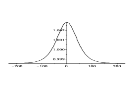
(a)

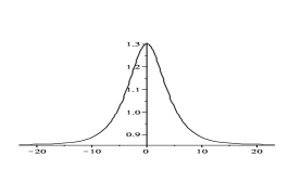
(b)

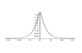
(c)

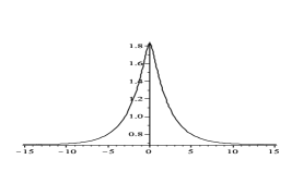
(d)

Figure 3: The solitons for Eq.(1.1). (a) $c=2$, $g=0.499999$; (b) $c=2$, $g=0.49$; (c) $c=2$, $g=0.46$ ; (d) $c=2$, $g=0.45$.

Note the following facts: when $g_{2}(c)<g<g_{1}(c)$ and $g$ tends to $g_{2}(c)$, the limit curve of such homoclinic orbit of system (2.3) is a triangle with the following three line segments (see Fig.2(b)):

$$y=\pm\frac{1}{2}(\varphi-c+\frac{4}{3})\quad for\quad\varphi_{1-}\leq\varphi\leq\varphi_{2},$$ (3.14)

and

$$\varphi=c\quad for\quad-\frac{2}{3}\leq y\leq\frac{2}{3}.$$ (3.15)

Let us have $g_{2}(c)<g<g_{1}(c)$ and $g$ tends to $g_{2}(c)$; then we obtain that

$$\varphi(\xi)=\frac{4}{3}\exp({-\frac{1}{2}|\xi|})+c-\frac{4}{3},$$ (3.16)

which implies that for arbitrary constant $c\neq 0$, Eq.(1.1) has peakons

$$u(x,t)=\frac{4}{3}\exp({-\frac{1}{2}|x-ct|})+(c-\frac{4}{3}).$$ (3.17)

Obviously, $u$ has peaks at $x-ct=0$. We show graphs of the peakons in Fig.4 under some parameter conditions.

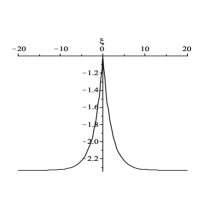
(a)

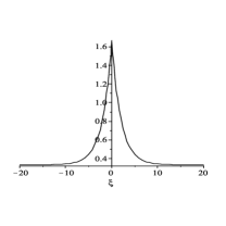
(b)

Figure 4: The peakons for Eq.(1.1). (a) $c=-1$ ; (b) $c=2$.

Remark 3.1

(1) If we take $c=\frac{4}{3}$ in (3.17), then we can see that (3.17) agrees with the result in [3].

(2) In the phase portaits, the triangle curve corresponds to a peakon solution.

We have the following lemma, similar to Lemma 3.1, which indicates the relationship of periodic wave solutions for Eq.(1.1) and periodic orbits of system (2.3).

Lemma 3.2

Assume that $\Gamma$ is a periodic orbit of system (2.3) and that its parameter expression is $\varphi=\varphi(\xi)$ and $y=y(\xi)$; then $u=\varphi(\xi)$ with $\xi=x-ct$ is a periodic wave solution for Eq.(1.1).

In Fig.2(c), the periodic orbit can be expressed as

$$y=\pm\sqrt{\frac{1}{4}\varphi^{2}-(\frac{1}{2}c-\frac{2}{3})\varphi-\frac{1}{4}c^{2}+\frac{1}{3}c+g}\quad for\quad\varphi_{2-}\leq\varphi\leq c,$$ (3.18)

and

$$\varphi=c\quad for\quad y_{1-}\leq y\leq y_{1+},$$ (3.19)

where

$$\varphi_{2-}=\frac{1}{3}(-4+3c+\sqrt{2(9c^{2}-18c+8-18g)}).$$ (3.20)

Substituting (3.18) into the first equation of system (2.3) and integrating along the periodic orbit, we have

$${\int_{\varphi}^{c}{\frac{1}{\sqrt{\varphi^{2}-(2c-\frac{8}{3})\varphi-c^{2}+\frac{4}{3}c+4g}}}ds=-\frac{1}{2}\xi}\quad for\quad\xi<0,$$ (3.21)

and

$${\int_{\varphi}^{c}{\frac{1}{\sqrt{\varphi^{2}-(2c-\frac{8}{3})\varphi-c^{2}+\frac{4}{3}c+4g}}}ds=\frac{1}{2}\xi}\quad for\quad\xi>0.$$ (3.22)

It follows from (3.21) and (3.22) that

$$\varphi(\xi)=l_{+}\exp({-\frac{1}{2}|\xi|})+l_{-}\exp({\frac{1}{2}|\xi|})+(c-\frac{4}{3})\quad for\quad\varphi_{2-}\leq\varphi\leq c,$$ (3.23)

where

$$l_{\pm}=\frac{1}{6}(4\pm 3\sqrt{4g+4c-2c^{2}}).$$ (3.24)

Let

$$T=2|\ln(\varphi_{2-}-c+\frac{4}{3})-\ln(2l_{-})|.$$ (3.25)

Then

$$u(x,t)=\varphi(x-ct-2nT)\quad for\quad(2n-1)T<x-ct<(2n+1)T,$$ (3.26)

are periodic cusp wave solutions for Eq.(1.1) with $2T$ period. Clearly, when $g_{3}(c)<g<g_{2}(c)$ and $g\rightarrow g_{2}(c)$, $T\rightarrow\infty$, $l_{+}\rightarrow\frac{3}{4}$, $l_{-}\rightarrow 0$, and $u(x,t)$ in (3.26) tends to

$$u(x,t)=\frac{4}{3}\exp({-\frac{1}{2}|x-ct|})+(c-\frac{4}{3}).$$ (3.27)

(3.27) is identical with (3.17). The graphs of some periodic waves for Eq.(1.1) are shown in Fig.5 under some parameter conditions. From Fig.5 we can see that $g_{3}(c)<g<g_{2}(c)$ and $g$ tends to $g_{2}(c)$, the periodic cusp wave solutions tend to peakons.

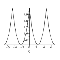
(a)

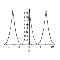
(b)

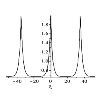
(c)

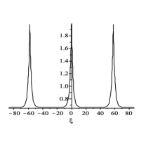
(d)

Figure 5: The periodic cusp wave solutions for Eq.(1.1). (a) $c=2$, $g=0.3$; (b) $c=2$, $g=0.4$; (c) $c=2$, $g=0.4444444$ ; (d) $c=2$, $g=0.444444444444$.

Remark 3.2

(1) In the phase portaits, the semi-elliptic closed curve with one side on the singular line $\varphi=c$ corresponds to a periodic cusp wave solution.

(2) In [4], we dealt with the case $g\leq g_{1}(c)$, and obtained the kink-like and antikink-like wave solutions for Eq.(1.1).

4 Conclusion

In this work, by using the bifurcation method, we obtain the analytic expressions for solitons, peakons and periodic wave solutions for the Fornberg-Whitham equation, given as (3.6), (3.17) and (3.26), respectively. We also show the relationships among the solitons, peakons and periodic cusp wave solutions.

References

- [1] G. B. Whitham, Variational methods and applications to water wave, Proc. R. Soc. Lond. Ser. A 299 (1967) 6-25.
- [2] R. Ivanov, On the integrability of a class of nonlinear dispersive wave equations, J. Nonlinear Math. Phys. 1294 (2005) 462-468.
- [3] B. Fornberg, G. B. Whitham, A numerical and theoretical study of certain nonlinear wave phenomena, Philos. Trans. R. Soc. Lond. Ser. A 289 (1978) 373-404.
- [4] J. Zhou, L. Tian, A type of bounded traveling wave solutions for the Fornberg-Whitham equation, J. Math. Anal. Appl. 346 (2008) 255-261.
- [5] D. Luo, et al., Bifurcation Theory and Methods of Dynamical Systems, World Scientific Publishing Co., London, 1997.