New exact travelling wave solutions for the $K(2,2)$ equation with osmosis dispersion

Abstract

In this paper, by using bifurcation method, we successfully find the $K(2,2)$ equation with osmosis dispersion $u_{t}+(u^{2})_{x}-(u^{2})_{xxx}=0$ possess two new types of travelling wave solutions called kink-like wave solutions and antikink-like wave solutions. They are defined on some semifinal bounded domains and possess properties of kink waves and anti-kink waves. Their implicit expressions are obtained. For some concrete data, the graphs of the implicit functions are displayed, and the numerical simulation of travelling wave system is made by Maple. The results show that our theoretical analysis agrees with the numerical simulation.

, ,

1 Introduction

In recent years, many nonlinear partial differential equations (NLPDEs) have been derived from physics, mechanics, engineering, biology, chemistry and other fields. Since exact solutions can help people know deeply the described process and possible applications, seeking exact solutions for NLPDEs is of great importance.

In 1993, Rosenau and Hyman [1] introduced a genuinely nonlinear dispersive equation, a special type of KdV equation, of the form

$$u_{t}+a(u^{n})_{x}+(u^{n})_{xxx}=0,n>1,$$ (1.1)

where $a$ is a constant and both the convection term $(u^{n})_{x}$ and the dispersion effect term $(u^{n})_{xxx}$ are nonlinear. These equations arise in the process of understanding the role of nonlinear dispersion in the formation of structures like liquid drops. Rosenau and Hyman derived solutions called compactons for Eq.(1.1) and showed that while compactons are the essence of the focusing branch where $a>0$, spikes, peaks, and cusps are the hallmark of the defocusing branch where $a<0$ which also supports the motion of kinks. Further, the negative branch, where $a<0$, was found to give rise to solitary patterns having cusps or infinite slopes. The focusing branch and the defocusing branch represent two different models, each leading to a different physical structure. Many powerful methods were applied to construct the exact solutions for Eq.(1.1), such as Adomain method [2], homotopy perturbation method [3], Exp-function method [4], variational iteration method [5], variational method [6, 7]. In [8], Wazwaz studied a generalized forms of the Eq.(1.1), that is $mK(n,n)$ equations and defined by

$$u^{n-1}u_{t}+a(u^{n})_{x}+b(u^{n})_{xxx}=0,n>1,$$ (1.2)

where $a,b$ are constants. He showed how to construct compact and noncompact solutions for Eq.(1.2) and discussed it in higher dimensional spaces in [9]. Chen et al. [10] showed how to construct the general solutions and some special exact solutions for Eq.(1.2) in higher dimensional spatial domains. He et al. [11] considered the bifurcation behavior of travelling wave solutions for Eq.(1.2). Under different parametric conditions, smooth and non-smooth periodic wave solutions, solitary wave solutions and kink and anti-kink wave solutions were obtained. Yan [12] further extended Eq.(1.2) to be a more general form

$$u^{m-1}u_{t}+a(u^{n})_{x}+b(u^{k})_{xxx}=0,nk\neq 1,$$ (1.3)

And using some direct ansatze, some abundant new compacton solutions, solitary wave solutions and periodic wave solutions of Eq.(1.3) were obtained. By using some transformations, Yan [13] obtained some Jacobi elliptic function solutions for Eq.(1.3). Biswas [14] obtained 1-soliton solution of equation with the generalized evolution term

$$(u^{l})_{t}+a(u^{m})u_{x}+b(u^{n})_{xxx}=0,$$ (1.4)

where $a,b$ are constants, while $l,m$ and $n$ are positive integers. Zhu et al. [15] applied the decomposition method and symbolic computation system to develop some new exact solitary wave solutions for the $K(2,2,1)$ equation

$$u_{t}+(u^{2})_{x}-(u^{2})_{xxx}+u_{xxxxx}=0,$$ (1.5)

and the $K(3,3,1)$ equation

$$u_{t}+(u^{3})_{x}-(u^{3})_{xxx}+u_{xxxxx}=0.$$ (1.6)

In [16], Xu and Tian introduced the osmosis $K(2,2)$ equation

$$u_{t}+(u^{2})_{x}-(u^{2})_{xxx}=0,$$ (1.7)

where the negative coefficient of dispersive term denotes the contracting dispersion. They obtained the peaked solitary wave solution and the periodic cusp wave solution for Eq.(1.7). In this paper, we’ll continue their work and using the bifurcation method of planar dynamical systems to derive two new types of bounded travelling wave solutions for Eq.(1.7). They are defined on some semifinal bounded domains and possess properties of kink waves and anti-kink waves. To our knowledge, such type of travelling wave solution has never been found for Eq.(1.7) in the former literature.

The remainder of the paper is organized as follows. In Section 2, we give the phase portrait of the travelling wave system and use Maple to show the graphs of the orbits connecting with the saddle points for our purpose. In Section 3, we state the main results which are implicit expressions of the kink-like and antikink-like wave solutions. In Section 4, we give the proof of the main results. For some concrete data, we use Maple to display the graphs of the implicit functions. In Section 5, the numerical simulations of travelling wave system are made by Maple. A short conclusion is given in Section 6.

2 Phase portrait of the travelling wave system

Eq.(1.7) also takes the form

$$u_{t}+2uu_{x}-6u_{x}u_{xx}-2uu_{xxx}=0,$$ (2.1)

Let $u=\varphi(\xi)$ with $\xi=x-ct(c\neq 0)$ be the solution for Eq.(2.1), then it follows that

$$-c\varphi^{\prime}+2\varphi\varphi^{\prime}-6\varphi^{\prime}\varphi^{\prime\prime}-2\varphi\varphi^{\prime\prime\prime}=0.$$ (2.2)

Integrating (2.2) once we have

$$-c\varphi+(\varphi)^{2}-2(\varphi^{\prime})^{2}-2\varphi\varphi^{\prime\prime}=g,$$ (2.3)

where $g$ is the integral constant.

Let $y=\varphi^{\prime}$, then we get the following planar dynamical system:

$$\left\{{\begin{array}[]{l}\frac{\textstyle d\varphi}{\textstyle d\xi}=y\\ \frac{\textstyle dy}{\textstyle d\xi}=\frac{\textstyle\varphi^{2}-c\varphi-g-2y^{2}}{\textstyle 2\varphi}\\ \end{array}}\right.$$ (2.4)

with a first integral

$$H(\varphi,y)=\varphi^{2}(y^{2}-\frac{1}{4}\varphi^{2}+\frac{c}{3}\varphi+\frac{1}{2}g)=h,$$ (2.5)

where $h$ is a constant.

Note that (2.4) has a singular line $\varphi=0$, to avoid the line temporarily we make transformation $d\xi=2\varphi d\zeta$. Under this transformation, Eq.(2.4) becomes

$$\left\{{\begin{array}[]{l}\frac{\textstyle d\varphi}{\textstyle d\zeta}=2\varphi y\\ \frac{\textstyle dy}{\textstyle d\zeta}=\varphi^{2}-c\varphi-g-2y^{2}\\ \end{array}}\right.$$ (2.6)

Eq.(2.4) and Eq.(2.6) have the same first integral as (2.5). Consequently, system (2.4) has the same topological phase portraits as system (2.6) except for the straight line $\varphi=0$. Obviously, $\varphi=0$ is an invariant straight-line solution for system (2.6).

Now we consider the singular points of system (2.6) and their properties. Note that for a fixed $h$, (2.5) determines a set of invariant curves of (2.6). As $h$ is varied, (2.5) determines different families of orbits of (2.6) having different dynamical behaviors. Let $M(\varphi_{e},y_{e})$ be the coefficient matrix of the linearized system of (2.6) at the equilibrium point $(\varphi_{e},y_{e})$, then

$$M(\varphi_{e},y_{e})=\left({{\begin{array}[]{*{20}c}{\indent y_{e}}&&&{\indent 2\varphi_{e}}\\ {2\varphi_{e}-c}&&&\indent{-4y_{e}}\\ \end{array}}}\right)$$

and at this equilibrium point, we have

$$J(\varphi_{e},y_{e})=\det M(\varphi_{e},y_{e})=-4y_{e}^{2}-4\varphi_{e}(\varphi_{e}-\frac{c}{2}\varphi_{e}),$$

$$p(\varphi_{e},y_{e})=\mathrm{trace}(M(\varphi_{e},y_{e}))=-3y_{e}.$$

By the theory of planar dynamical system (see [17]), for an equilibrium point of a planar dynamical system, if $J<0$, then this equilibrium point is a saddle point; it is a center point if $J>0$ and $p=0$; if $J=0$ and the Poincáre index of the equilibrium point is 0, then it is a cusp.

Although the distribution and properties of equilibrium points of system (2.4) has been given in [16]. Here we also state it briefly for our purpose. System (2.4) has the following properties:

(1) When $g>0$, system (2.4) has two equilibrium points $(\varphi_{0}^{-},0)$ and $(\varphi_{0}^{+},0)$. They are saddle points. (i) If $c<0$, then there is inequality $\varphi_{0}^{-}<\frac{c}{2}<0<\varphi_{0}^{+}$; (ii) If $c>0$, then there is inequality $\varphi_{0}^{-}<0<\frac{c}{2}<\varphi_{0}^{+}$.

(2) When $g=0$, system (2.4) has two equilibrium points $(0,0)$ and $(c,0)$. $(0,0)$ is a cusp, and $(c,0)$ is a saddle point.

(3) When $-\frac{c^{2}}{4}<g<0$, system (2.4) has two equilibrium points $(\varphi_{0}^{-},0)$ and $(\varphi_{0}^{+},0)$. (i) If $c<0$, then $(\varphi_{0}^{-},0)$ is a saddle point while $(\varphi_{0}^{+},0)$ is a center point. There is inequality $\varphi_{0}^{-}<\frac{c}{2}<\varphi_{0}^{+}<0$; (ii) If $c>0$ , then $(\varphi_{0}^{-},0)$ is a center point while $(\varphi_{0}^{+},0)$ is a saddle point. There is inequality $0<\varphi_{0}^{-}<\frac{c}{2}<\varphi_{0}^{+}$.

(4) When $g=-\frac{c^{2}}{4}$, system (2.4) has only one equilibrium point $(\frac{c}{2},0)$. It is a cusp.

(5) When $g<-\frac{c^{2}}{4}$, system (2.4) has no equilibrium point.

Remark 2.1

Suppose that $\varphi(\xi)(\xi=x-ct)$ is a travelling wave solution for Eq.(1.7) for $\xi\in(-\infty,+\infty)$, and $\mathop{\lim}\limits_{\xi\to-\infty}\varphi(\xi)=A$, $\mathop{\lim}\limits_{\xi\to\infty}\varphi(\xi)=B$, where $A$ and $B$ are two constants. If $A=B$, then $\varphi(\xi)$ is called a solitary wave solution. If $A\neq B$, then $\varphi(\xi)$ is called a kink (or an anti-kink) solution. Usually, a solitary wave solution for Eq.(1.7) corresponds to a homoclinic orbit of system (2.6) and a periodic orbit of system (2.6) corresponds to a periodic travelling wave solution of Eq.(1.7). Similarly, a kink (or an anti-kink) wave solution of Eq.(1.7) corresponds to a heteroclinic orbit (or so-called connecting orbit) of system (2.6). In [16], Xu and Tian reported that when $-\frac{c^{2}}{4}<g<-\frac{2c^{2}}{9}$, system (2.6) has homoclinic orbits, and when $-\frac{c^{2}}{4}<g<0$, system (2.6) has a periodic orbit which consist of an arc and a line segment. They obtained peakon solutions from the limit of solitary waves and from the limit of periodic cusp waves. We’ll obtain a new type of bounded travelling wave solutions called kink-like and antikink-like wave solutions for Eq.(1.7) when $g>-\frac{2c^{2}}{9}$, which correspond to the orbits of system (2.6) connecting with the saddle points.

We show the phase portraits in each region and on the bifurcation curves in Fig.1. From Fig.1, we can see that when $g>-\frac{2c^{2}}{9}$, system (2.6) has orbits connecting with the saddle points.

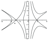
(a)

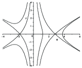
(b)

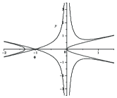
(c)

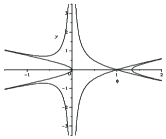
(d)

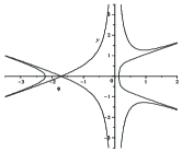
(e)

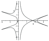
(f)

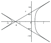
(g)

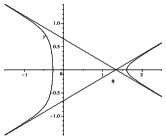
(h)

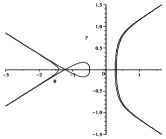
(i)

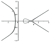
(j)

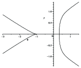
(k)

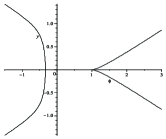
(l)

Figure 1: Phase portrait of system (2.6). (a) $g>0$, $c<0$; (b) $g>0$, $c>0$; (c) $g=0$, $c<0$; (d) $g=0$, $c>0$; (e) $-\frac{2c^{2}}{9}<g<0$, $c<0$; (f) $-\frac{2c^{2}}{9}<g<0$, $c>0$; (g) $g=-\frac{2c^{2}}{9}$, $c<0$; (h) $g=-\frac{2c^{2}}{9}$, $c>0$; (i) $-\frac{c^{2}}{4}<g<-\frac{2c^{2}}{9}$, $c<0$; (j) $-\frac{c^{2}}{4}<g<-\frac{2c^{2}}{9}$, $c>0$; (k) $g=-\frac{c^{2}}{4}$, $c<0$; (l) $g=-\frac{c^{2}}{4}$, $c>0$.

3 Main results

We state our main result as follows.

Theorem 3.1

For given constant $c\neq 0$, let

$$\xi=x-ct,$$ (3.1)

$$\varphi_{0}^{\pm}=\frac{c\pm\sqrt{c^{2}+4g}}{2},$$ (3.2)

(1) When $g>0$ and $c<0$, Eq.(1.7) has two kink-like wave solutions $u=\varphi_{1}(\xi)$ and $u=\varphi_{3}(\xi)$ and two antikink-like wave solutions $u=\varphi_{2}(\xi)$ and $u=\varphi_{4}(\xi)$.

$$\beta_{1}(\varphi_{1})=\beta_{1}(a)\exp(-\frac{1}{2}\xi),\\ \quad\xi\in(-\infty,\xi_{0}^{1}),$$ (3.3)

$$\beta_{1}(\varphi_{2})=\beta_{1}(a)\exp(\frac{1}{2}\xi),\\ \quad\quad\xi\in(-\xi_{0}^{1},\infty),$$ (3.4)

$$\beta_{2}(\varphi_{3})=\beta_{2}(b)\exp(-\frac{1}{2}\xi),\\ \quad\quad\xi\in(-\xi_{0}^{3},\infty),$$ (3.5)

$$\beta_{2}(\varphi_{4})=\beta_{2}(b)\exp(\frac{1}{2}\xi),\\ \quad\quad\xi\in(-\infty,\xi_{0}^{3}),$$ (3.6)

(2) When $g>0$ and $c>0$, Eq.(1.7) has two kink-like wave solutions $u=\varphi_{1}(\xi)$ and $u=\varphi_{3}(\xi)$ and two antikink-like wave solutions $u=\varphi_{2}(\xi)$ and $u=\varphi_{4}(\xi)$.

$$\beta_{1}(\varphi_{1})=\beta_{1}(a)\exp(-\frac{1}{2}\xi),\\ \quad\xi\in(-\infty,\xi_{0}^{5}),$$ (3.7)

$$\beta_{1}(\varphi_{2})=\beta_{1}(a)\exp(\frac{1}{2}\xi),\\ \quad\quad\xi\in(-\xi_{0}^{5},\infty),$$ (3.8)

$$\beta_{2}(\varphi_{3})=\beta_{2}(b)\exp(-\frac{1}{2}\xi),\\ \quad\quad\xi\in(-\xi_{0}^{7},\infty),$$ (3.9)

$$\beta_{2}(\varphi_{4})=\beta_{2}(b)\exp(\frac{1}{2}\xi),\\ \quad\quad\xi\in(-\infty,\xi_{0}^{7}),$$ (3.10)

(3) When $-\frac{2c^{2}}{9}<g\leq 0$ and $c<0$, Eq.(1.7) has a kink-like wave solution $u=\varphi_{5}(\xi)$ and an antikink-like wave solution $u=\varphi_{6}(\xi)$.

$$\beta_{1}(\varphi_{5})=\beta_{1}(d)\exp(-\frac{1}{2}\xi),\\ \quad\xi\in(-\infty,\xi_{0}^{9}),$$ (3.11)

$$\beta_{1}(\varphi_{6})=\beta_{1}(d)\exp(\frac{1}{2}\xi),\\ \quad\quad\xi\in(-\xi_{0}^{9},\infty),$$ (3.12)

(4) When $-\frac{2c^{2}}{9}<g\leq 0$ and $c>0$, Eq.(1.7) has a kink-like wave solution $u=\varphi_{7}(\xi)$ and an antikink-like wave solution $u=\varphi_{8}(\xi)$.

$$\beta_{2}(\varphi_{7})=\beta_{2}(k)\exp(-\frac{1}{2}\xi),\\ \quad\xi\in(-\infty,\xi_{0}^{11}),$$ (3.13)

$$\beta_{2}(\varphi_{8})=\beta_{2}(k)\exp(\frac{1}{2}\xi),\\ \quad\quad\xi\in(-\xi_{0}^{11},\infty),$$ (3.14)

where

$$\varphi_{1}^{*}=\frac{c-\sqrt{c^{2}+3g}}{2},$$ (3.15)

$$\varphi_{2}^{*}=\frac{c+\sqrt{c^{2}+3g}}{2},$$ (3.16)

$$l_{1}=-\frac{1}{3}(c+3\sqrt{c^{2}+4g}),$$ (3.17)

$$l_{2}=\frac{1}{6}(c^{2}+6g-c\sqrt{c^{2}+4g}),$$ (3.18)

$$l_{3}=\frac{2}{3}(c^{2}+6g-c\sqrt{c^{2}+4g}),$$ (3.19)

$$m_{1}=-\frac{1}{3}(c-3\sqrt{c^{2}+4g}),$$ (3.20)

$$m_{2}=\frac{1}{6}(c^{2}+6g+c\sqrt{c^{2}+4g}),$$ (3.21)

$$m_{3}=\frac{2}{3}(c^{2}+6g+c\sqrt{c^{2}+4g}),$$ (3.22)

$$a_{1}=c^{2}+4g-c\sqrt{c^{2}+4g},$$ (3.23)

$$a_{2}=c^{2}+4g+c\sqrt{c^{2}+4g},$$ (3.24)

$$b_{1}=\frac{1}{3}(2c-6\sqrt{c^{2}+4g}),$$ (3.25)

$$b_{2}=\frac{1}{3}(2c+6\sqrt{c^{2}+4g}),$$ (3.26)

$$\alpha_{1}=\frac{c-\sqrt{c^{2}+4g}}{2\sqrt{c^{2}+4g-c\sqrt{c^{2}+4g}}},$$ (3.27)

$$\alpha_{2}=\frac{c+\sqrt{c^{2}+4g}}{2\sqrt{c^{2}+4g+c\sqrt{c^{2}+4g}}},$$ (3.28)

$$\beta_{1}(\varphi)=\frac{(2\sqrt{\varphi^{2}+l_{1}\varphi+l_{2}}+2\varphi+l_{1})(\varphi-\varphi_{0}^{-})^{\alpha_{1}}}{(2\sqrt{a_{1}}\sqrt{\varphi^{2}+l_{1}\varphi+l_{2}}+b_{1}\varphi+l_{3})^{\alpha_{1}}},$$ (3.29)

$$\beta_{2}(\varphi)=\frac{(2\sqrt{\varphi^{2}+m_{1}\varphi+m_{2}}+2\varphi+m_{1})(\varphi-\varphi_{0}^{+})^{\alpha_{2}}}{(2\sqrt{a_{2}}\sqrt{\varphi^{2}+m_{1}\varphi+m_{2}}+b_{2}\varphi+m_{3})^{\alpha_{2}}},$$ (3.30)

$$\xi_{0}^{1}=2\ln(\beta_{1}(a)/\beta_{1}(\frac{c}{2})),$$ (3.31)

$$\xi_{0}^{3}=2\ln(\beta_{2}(\varphi_{2}^{*})/\beta_{2}(b))$$ (3.32)

$$\xi_{0}^{5}=2\ln(\beta_{1}(a)/\beta_{1}(\varphi_{1}^{*})),$$ (3.33)

$$\xi_{0}^{7}=2\ln(\beta_{2}(\frac{c}{2})/\beta_{2}(b)),$$ (3.34)

$$\xi_{0}^{9}=2\ln(\beta_{1}(d)/\beta_{1}(\frac{c}{2})),$$ (3.35)

$$\xi_{0}^{11}=2\ln(\beta_{2}(\frac{c}{2})/\beta_{2}(k)),$$ (3.36)

$a$, $b$, $d$, $k$ are four constants satisfying $\varphi_{1}(0)=\varphi_{2}(0)=a$, $\varphi_{3}(0)=\varphi_{4}(0)=b$, $\varphi_{5}(0)=\varphi_{6}(0)=d$, $\varphi_{7}(0)=\varphi_{8}(0)=k$, and there are inequalities $\varphi_{0}^{-}<a<\frac{c}{2}<0<\varphi_{2}^{*}<b<\varphi_{0}^{+}$ for $c<0$, $\varphi_{0}^{-}<a<\varphi_{1}^{*}<0<\frac{c}{2}<b<\varphi_{0}^{+}$ for $c>0$, $\varphi_{0}^{-}<d<\frac{c}{2}<\varphi_{0}^{+}<0$ for $c<0$ and $0<\varphi_{0}^{-}<\frac{c}{2}<k<\varphi_{0}^{+}$ for $c>0$.

We will give the proof of this theorem in Section 4. Now we take a set of data and employ Maple to display the graphs of $u=\varphi_{i}(\xi)(i=1,2,3,4,5,6,7,8)$.

Example 3.1

Taking $g=5$, $c=-1$ (corresponding to (1) in Theorem (3.1)), it follows that $\varphi_{0}^{-}=-2.79129$ , $\varphi_{0}^{+}=1.79129$, $l_{1}=-4.24924$, $l_{2}=5.93043$, $l_{3}=23.7217$, $a_{1}=25.5826$, $b_{1}=-9.83182$ , $\alpha_{1}=-0.551865$. Further, choosing $a=-0.75\in(\varphi_{0}^{-},\frac{c}{2})$, we obtain $\xi_{0}^{1}=0.0482492$. We present the graphs of the solutions $\varphi_{1}(\xi)$ and $\varphi_{2}(\xi)$ in Fig.2 (a) and (b), respectively. Meanwhile, we get $m_{1}=4.51591$, $m_{2}=4.4029$, $m_{3}=17.6116$, $a_{2}=16.4174$, $b_{2}=8.49848$, $\alpha_{2}=0.442092$, $\varphi_{2}^{*}=1.5$. Further, choosing $b=1.6\in(\varphi_{2}^{*},\varphi_{0}^{+})$, we get $\xi_{0}^{3}=0.343656$. The graphs of the solutions $\varphi_{3}(\xi)$ and $\varphi_{4}(\xi)$ are presented in Fig.2(c) and (d), respentively. The graphs in Fig.2 show that $\varphi_{1}(\xi)$ and $\varphi_{3}(\xi)$ are two kink-like wave solutions and $\varphi_{2}(\xi)$ and $\varphi_{4}(\xi)$ are two antikink-like wave solutions.

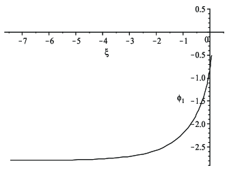
(a)

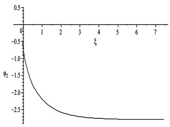
(b)

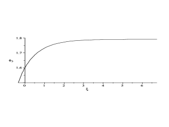
(c)

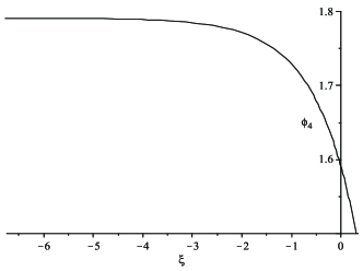
(d)

Figure 2: The graphs of $\varphi_{i}(\xi)(i=1,2,3,4)$ when $g=5$, $c=-1$, $a=-0.75$, $b=1.6$.

Example 3.2

Taking $g=5$, $c=1$ (corresponding to (2) in Theorem (3.1)), it follows that $\varphi_{0}^{-}=-1.79129$ , $\varphi_{0}^{+}=2.79129$, $l_{1}=-4.51591$, $l_{2}=4.4029$, $l_{3}=17.6116$, $a_{1}=16.4174$, $b_{1}=-8.49848$ , $\alpha_{1}=-0.442092$, $\varphi_{1}^{*}=-1.5$. Further, choosing $a=-1.6\in(\varphi_{0}^{-},\varphi_{1}^{*})$, we obtain $\xi_{0}^{5}=0.343656$. We present the graphs of the solutions $\varphi_{1}(\xi)$ and $\varphi_{2}(\xi)$ in Fig.3 (a) and (b), respectively. Meanwhile, we get $m_{1}=4.249241$, $m_{2}=5.93043$, $m_{3}=23.7214$, $a_{2}=25.58264$, $b_{2}=9.93182$, $\alpha_{2}=0.551865$. Further, choosing $b=2\in(\frac{c}{2},\varphi_{0}^{+})$, we get $\xi_{0}^{7}=0.773847$. The graphs of the solutions $\varphi_{3}(\xi)$ and $\varphi_{4}(\xi)$ are presented in Fig.3(c) and (d), respentively. The graphs in Fig.3 show that $\varphi_{1}(\xi)$ and $\varphi_{3}(\xi)$ are two kink-like wave solutions and $\varphi_{2}(\xi)$ and $\varphi_{4}(\xi)$ are two antikink-like wave solutions.

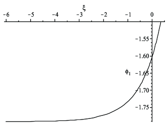
(a)

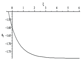
(b)

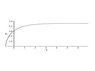
(c)

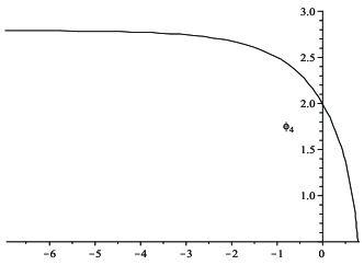
(d)

Figure 3: The graphs of $\varphi_{i}(\xi)(i=1,2,3,4)$ when $g=5$, $c=1$, $a=-1.6$, $b=2$.

Example 3.3

Taking $g=-0.5$, $c=-2$ (corresponding to (3) in Theorem (3.1)), it follows that $\varphi_{0}^{-}=-1.70711$ , $\varphi_{0}^{+}=-0.292893$, $l_{1}=-0.747547$, $l_{2}=0.638071$, $l_{3}=2.5528$, $a_{1}=4.82843$, $b_{1}=-4.16176$ , $\alpha_{1}=-0.776887$. Further, choosing $d=-1.2\in(\varphi_{0}^{-},\frac{c}{2})$, we obtain $\xi_{0}^{9}=0.448123$. We present the graphs of the solutions $\varphi_{5}(\xi)$ and $\varphi_{6}(\xi)$ in Fig.4 (a) and (b), respectively. The graphs in Fig.4 show that $\varphi_{5}(\xi)$ is a kink-like wave solution and $\varphi_{6}(\xi)$ is an antikink-like wave solution.

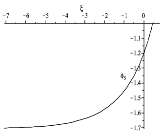
(a)

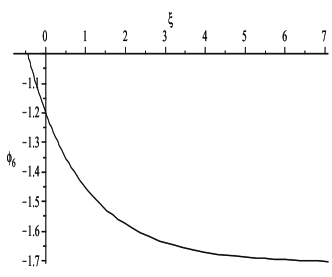
(b)

Figure 4: The graphs of $\varphi_{i}(\xi)(i=5,6)$ when $g=-0.5$, $c=-2$, $d=-1.2$.

Example 3.4

Taking $g=-0.5$, $c=2$ (corresponding to (4) in Theorem (3.1)), it follows that $\varphi_{0}^{-}=0.292893$ , $\varphi_{0}^{+}=1.70711$, $m_{1}=0.747547$, $m_{2}=0638071$, $m_{3}=2.55228$, $a_{2}=4.82843$, $b_{2}=4.1676$, $\alpha_{2}=0.776887$. Further, choosing $k=1.2\in(\frac{c}{2},\varphi_{0}^{+})$, we get $\xi_{0}^{11}=0.448123$. The graphs of the solutions $\varphi_{7}(\xi)$ and $\varphi_{8}(\xi)$ are presented in Fig.5 (a) and (b), respentively. The graphs in Fig.5 show that $\varphi_{7}(\xi)$ is a kink-like wave solutions and $\varphi_{8}(\xi)$ is an antikink-like wave solutions.

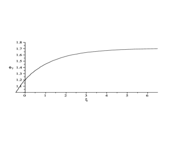
(a)

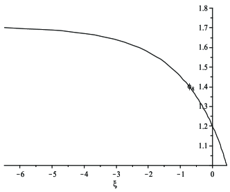
(b)

Figure 5: The graphs of $\varphi_{i}(\xi)(i=7,8)$ when $g=-0.5$, $c=2$, $k=1.2$.

4 Proof of main results

Suppose $g>0$ and $c<0$, then system (2.4) has two saddle points $(\varphi_{0}^{-},0)$ and $(\varphi_{0}^{+},0)$. There are four orbits connecting with $(\varphi_{0}^{-},0)$. We use $l_{\varphi_{0}^{-}}^{2}$ to denote the two orbits lying on the right side of $(\varphi_{0}^{-},0)$ (see Fig.6(a)). Meanwhile, there are four orbits connecting with $(\varphi_{0}^{+},0)$. We employ $l_{\varphi_{0}^{+}}^{1}$ and $l_{\varphi_{0}^{+}}^{2}$ to denote the two orbits lying on the left side of $(\varphi_{0}^{+},0)$ (see Fig.6(a)).

(a)

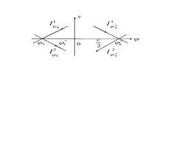
(b)

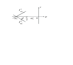
(c)

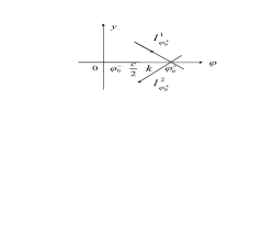
(d)

Figure 6: The sketches of orbits connecting with saddle points. (a)$g>0$, $c<0$; (b)$g>0$, $c>0$; (c) $-\frac{2c^{2}}{9}<g\leq 0$, $c<0$; (d)$-\frac{2c^{2}}{9}<g\leq 0$, $c>0$.

On the $\varphi-y$ plane, the orbits $l_{\varphi_{0}^{-}}^{1}$, $l_{\varphi_{0}^{-}}^{2}$, $l_{\varphi_{0}^{+}}^{1}$ and $l_{\varphi_{0}^{+}}^{2}$ have the following expressions, respectively,

$$l_{\varphi_{0}^{-}}^{1}:\quad y=\frac{(\varphi_{0}^{-}-\varphi)\sqrt{\varphi^{2}+l_{1}\varphi+l_{2}}}{2\varphi}$$ (4.1)

$$l_{\varphi_{0}^{-}}^{2}:\quad y=\frac{(\varphi-\varphi_{0}^{-})\sqrt{\varphi^{2}+l_{1}\varphi+l_{2}}}{2\varphi}$$ (4.2)

$$l_{\varphi_{0}^{+}}^{1}:\quad y=\frac{(\varphi_{0}^{+}-\varphi)\sqrt{\varphi^{2}+m_{1}\varphi+m_{2}}}{2\varphi}$$ (4.3)

$$l_{\varphi_{0}^{+}}^{2}:\quad y=\frac{(\varphi-\varphi_{0}^{+})\sqrt{\varphi^{2}+m_{1}\varphi+m_{2}}}{2\varphi}$$ (4.4)

where $\varphi_{0}^{-}$ and $\varphi_{0}^{+}$ are in (3.2) , $l_{1}$ and $l_{2}$ are in (3.17) and (3.18), $m_{1}$ and $m_{2}$ are in (3.20) and (3.21), respectively.

Assume that $\varphi=\varphi_{1}(\xi)$, $\varphi=\varphi_{2}(\xi)$, $\varphi=\varphi_{3}(\xi)$ and $\varphi=\varphi_{4}(\xi)$ on $l_{\varphi_{0}^{-}}^{1}$, $l_{\varphi_{0}^{-}}^{2}$, $l_{\varphi_{0}^{+}}^{1}$ and $l_{\varphi_{0}^{+}}^{2}$, respectively and $\varphi_{1}(0)=\varphi_{2}(0)=a$, $\varphi_{3}(0)=\varphi_{4}(0)=b$, $\varphi_{2}^{*}=\frac{c+\sqrt{c^{2}+3g}}{2}$, where $a$ and $b$ are two constants satisfying $\varphi_{0}^{-}<a<\frac{c}{2}$ and $\varphi_{2}^{*}<b<\varphi_{0}^{+}$. Substituting (4.1)-(4.4) into the first equation of (2.4) and integrating along the corresponding orbits, respectively, we have

$$\int_{a}^{\varphi_{1}}{\frac{-s}{(s-\varphi_{0}^{-})\sqrt{s^{2}+l_{1}s+l_{2}}}ds=\frac{1}{2}\int_{0}^{\xi}{ds}}\quad\quad(\textmd{along}\quad l_{\varphi_{0}^{-}}^{1}),$$ (4.5)

$$\int_{\varphi_{2}}^{a}{\frac{s}{(s-\varphi_{0}^{-})\sqrt{s^{2}+l_{1}s+l_{2}}}ds=\frac{1}{2}\int_{\xi}^{0}{ds}}\quad\quad(\textmd{along}\quad l_{\varphi_{0}^{-}}^{2}),$$ (4.6)

$$\int_{\varphi_{3}}^{b}{\frac{-s}{(s-\varphi_{0}^{+})\sqrt{s^{2}+m_{1}s+m_{2}}}ds=\frac{1}{2}\int_{\xi}^{0}{ds}}\quad(\textmd{along}\quad l_{\varphi_{0}^{+}}^{1}),$$ (4.7)

$$\int_{b}^{\varphi_{4}}{\frac{s}{(s-\varphi_{0}^{+})\sqrt{s^{2}+m_{1}s+m_{2}}}ds=\frac{1}{2}\int_{0}^{\xi}{ds}}\quad(\textmd{along}\quad l_{\varphi_{0}^{+}}^{2}).$$ (4.8)

With the aim of Maple, we obtain the implicit expressions of $\varphi_{i}(\xi)$ as in (3.3)-(3.6).

Meanwhile, suppose that $\varphi_{1}(\xi)\to\frac{c}{2}$ as $\xi\to\xi_{0}^{1}$, $\varphi_{2}(\xi)\to\frac{c}{2}$ as $\xi\to-\xi_{0}^{2}$, $\varphi_{3}(\xi)\to\varphi_{2}^{*}$ as $\xi\to-\xi_{0}^{3}$ and $\varphi_{4}(\xi)\to\varphi_{2}^{*}$ as $\xi\to\xi_{0}^{4}$, then it follow from (4.5) -(4.8) that

$$\xi_{0}^{1}=\xi_{0}^{2}=\int_{a}^{\frac{c}{2}}{\frac{-s}{(s-\varphi_{0}^{-})\sqrt{s^{2}+l_{1}s+l_{2}}}ds}\quad\quad(\textmd{along}\quad l_{\varphi_{0}^{-}}^{1}),$$ (4.9)

$$\xi_{0}^{3}=\xi_{0}^{4}=\int_{b}^{\varphi_{2}^{*}}{\frac{s}{(s-\varphi_{0}^{+})\sqrt{s^{2}+m_{1}s+m_{2}}}ds}\quad(\textmd{along}\quad l_{\varphi_{0}^{+}}^{2}).$$ (4.10)

With the aim of Maple, we get the expressions of $\xi_{0}^{1}$ and $\xi_{0}^{3}$ as in (3.31) and (3.32). The proof of (1) in Theorem (3.1) is finished.

Similarly, we can prove (2)-(4) in Theorem (3.1). Here we omit the details.

5 Numerical simulations

In this section, we will simulate the planar graphs of the kink-like and antikink-like wave solutions.

From Section 2, we see that in the parameter expressions $\varphi=\varphi(\xi)$ and $y=y(\xi)$ of the orbits of system (2.6), the graph of $\varphi(\xi)$ and the integral curve of Eq.(2.3) are the same. In other words, the integral curves of Eq.(2.3) are the planar graphs of the traveling waves of Eq.(1.7). Therefore, we can see the planar graphs of the kink-like and the antikink-like waves through the simulation of the integral curves of Eq.(2.3).

Example 5.1

Take the same data as Example (3.1), that is $g=5$, $c=-1$, $a=-0.75$, $b=1.6$. Let $\varphi=a=-0.75$ in (4.1) and (4.2), then we can get $y\approx 4.23397$ or $y\approx-4.23397$. And let $\varphi=b=1.6$ in (4.3) and (4.4), then we obtain $y\approx 0.23198$ or $y\approx-0.23198$. Thus we take the initial conditions of Eq.(2.3) as follows: (a) Corresponding to $l_{\varphi_{0}^{-}}^{1}$ we take $\varphi(0)=-0.75$ and $\varphi^{\prime}(0)=4.23397$; (b) Corresponding to $l_{\varphi_{0}^{-}}^{2}$ we take $\varphi(0)=-0.75$ and $\varphi^{\prime}(0)=-4.23397$; (c) Corresponding to $l_{\varphi_{0}^{+}}^{1}$ we take $\varphi(0)=1.6$ and $\varphi^{\prime}(0)=0.23198$; (d) Corresponding to $l_{\varphi_{0}^{+}}^{2}$ we take $\varphi(0)=1.6$ and $\varphi^{\prime}(0)=-0.23198$. Under each set of initial conditions we use Maple to simulate the integrals curve of Eq.(2.3) in Fig.7.

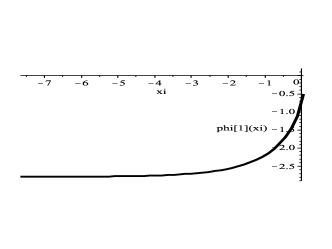
(a)

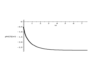
(b)

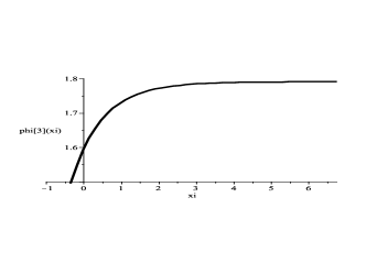
(c)

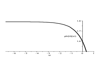
(d)

Figure 7: The numerical simulations of integral curves of Eq.(2.3) when $g=5$ and $c=-1$. (a) $\varphi(0)=-0.75$, $\varphi^{\prime}(0)=4.23397$; (b) $\varphi(0)=-0.75$, $\varphi^{\prime}(0)=-4.23397$; (c) $\varphi(0)=1.6$, $\varphi^{\prime}(0)=0.230189$; (d) $\varphi(0)=1.6$, $\varphi^{\prime}(0)=-0.230189$.

Example 5.2

Take the same data as Example (3.2), that is $g=5$, $c=1$, $a=-1.6$, $b=2$. Let $\varphi=a=-1.6$ in (4.1) and (4.2) , then we can get $y\approx 0.230189$ or $y\approx-0.230189$. And let $\varphi=b=2$ in (4.3) and (4.4), then we obtain $y\approx 0.849228$ or $y\approx-0.849228$. Thus we take the initial conditions of Eq.(2.3) as follows: (a) Corresponding to $l_{\varphi_{0}^{-}}^{1}$ we take $\varphi(0)=-1.6$ and $\varphi^{\prime}(0)=0.230189$; (b) Corresponding to $l_{\varphi_{0}^{-}}^{2}$ we take $\varphi(0)=-1.6$ and $\varphi^{\prime}(0)=-0.230189$; (c) Corresponding to $l_{\varphi_{0}^{+}}^{1}$ we take $\varphi(0)=2$ and $\varphi^{\prime}(0)=0.849228$; (d) Corresponding to $l_{\varphi_{0}^{+}}^{2}$ we take $\varphi(0)=2$ and $\varphi^{\prime}(0)=-0.849228$. Under each set of initial conditions we use Maple to simulate the integrals curve of Eq.(2.3) in Fig.8.

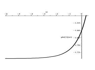
(a)

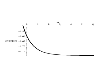
(b)

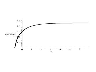
(c)

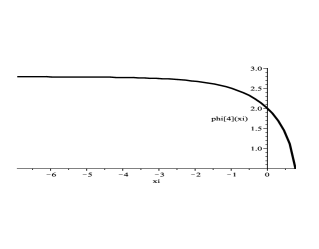
(d)

Figure 8: The numerical simulations of integral curves of Eq.(2.3) when $g=5$ and $c=1$. (a) $\varphi(0)=-1.6$, $\varphi^{\prime}(0)=0.230189$; (b) $\varphi(0)=-1.6$, $\varphi^{\prime}(0)=-0.230189$; (c) $\varphi(0)=2$, $\varphi^{\prime}(0)=0.849228$; (d) $\varphi(0)=2$, $\varphi^{\prime}(0)=-0.849228$.

Example 5.3

Take the same data as Example (3.3), that is $g=-0.5$, $c=-2$, $d=-1.2$. Let $\varphi=d=-1.2$ in (4.1) and (4.2), then we can get $y\approx 0.364453$ or $y\approx-0.364453$. Thus we take the initial conditions of Eq.(2.3) as follows: (a) Corresponding to $l_{\varphi_{0}^{-}}^{1}$ we take $\varphi(0)=-1.2$ and $\varphi^{\prime}(0)=0.364453$; (b) Corresponding to $l_{\varphi_{0}^{-}}^{2}$ we take $\varphi(0)=-1.2$ and $\varphi^{\prime}(0)=-0.364453$. Under each set of initial conditions we use Maple to simulate the integrals curve of Eq.(2.3) in Fig.9.

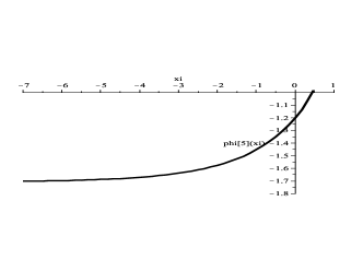
(a)

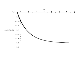
(b)

Figure 9: The numerical simulations of integral curves of Eq.(2.3) when $g=-0.5$ and $c=-2$. (a) $\varphi(0)=-1.6$, $\varphi^{\prime}(0)=0.230189$; (b) $\varphi(0)=-1.6$, $\varphi^{\prime}(0)=-0.230189$.

Example 5.4

Take the same data as Example (3.4), that is $g=-0.5$, $c=2$, $k=1.2$. Let $\varphi=k=-1.6$ in (4.3) and (4.4) , then we can get $y\approx 0.364453$ or $y\approx-0.364453$. Thus we take the initial conditions of Eq.(2.3) as follows: (a) Corresponding to $l_{\varphi_{0}^{+}}^{1}$ we take $\varphi(0)=1.2$ and $\varphi^{\prime}(0)=0.364453$; (b) Corresponding to $l_{\varphi_{0}^{+}}^{2}$ we take $\varphi(0)=1.2$ and $\varphi^{\prime}(0)=-0.364453$. Under each set of initial conditions we use Maple to simulate the integrals curve of Eq.(2.3) in Fig.10.

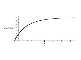
(a)

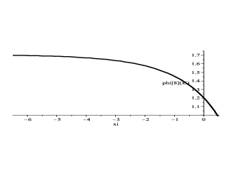
(b)

Figure 10: The numerical simulations of integral curves of Eq.(2.3) when $g=-0.5$ and $c=2$. (a) $\varphi(0)=1.2$, $\varphi^{\prime}(0)=0.364453$; (b) $\varphi(0)=1.2$, $\varphi^{\prime}(0)=-0.364453$.

Comparing Fig.2 with Fig.7, Fig.3 with Fig.8, Fig.4 with Fig.9, and Fig.5 with Fig.10, we can see that the graphs of $\varphi_{i}(\xi)(i=1,2,3,4,5,6,7,8)$ are the same as the corresponding integral curves of Eq.(2.3). This implies that our theoretical results agree with the numerical simulations.

6 Conclusion

In this paper, we find a new type of bounded travelling wave solutions for the $K(2,2)$ equation with osmosis dispersion. Their implicit expressions are obtained in (3.3)-(3.14). From the graphs (see Fig.2-Fig.5) of the implicit functions and the numerical simulations (see Fig.7-Fig.10) we see that these new bounded solutions are defined on some semifinal bounded domains and possess properties of kink and anti-kink wave solutions.

References

- [1] P. Rosenau, J. M. Hyman, Compactons: solitons with finite wavelengths, Phys. Rev. Lett. 70 (5) (1993) 564-567.
- [2] A. M. Wazwaz, Compactons and solitary patterns structures for variants of the KdV and the KP equations, Appl. Math. Comput. 138 (2/3) (2003) 309-319.
- [3] J. H. He, Homotopy perturbation method for bifurcation of nonlinear problems, Int. J Nonlinear Sci. Numer. Simulat. 6 (2) (2005) 207-208.
- [4] J. H. He, X. H. Wu, Exp-function method for nonlinear wave equations, Chaos, Solitons and Fractals 30 (3) (2006) 700-708.
- [5] J. H. He, X. H. Wu, Construction of solitary solution and compacton-like solution by variational iteration method, Chaos, Solitons and Fractals 29 (1) (2006) 108-113.
- [6] J. H. He, Some asymptotic methods for strongly nonlinear equations, Int. J Modern Phys. B 20 (10) (2006) 1141-1199.
- [7] L. Xu, Variational approach to solitons of nonlinear dispersive equations, Chaos, Solitons and Fractals 37 (1) (2008) 137-143.
- [8] A. M. Wazwaz, General compacts solitary patterns solutions for modified nonlinear dispersive equation in higher dimensional spaces, Math. Comput. Simulat. 59 (6) (2002) 519-531.
- [9] A. M. Wazwaz, Compact and noncompact structures for a variant of KdV equation in higher dimensions, Appl. Math. Comput. 132 (1) (2002) 29-45.
- [10] Y. Chen, B. Li, H. Q. Zhang, New exact solutions for modified nonlinear dispersive equations in higher dimensions spaces, Math. Comput. Simul. 64 (5) (2004) 549-559.
- [11] B. He, Q. Meng, W. Rui , Y. Long, Bifurcations of travelling wave solutions for the equation, Commun. Nonlinear Sci. Numer. Simulat. 13 (2008) 2114-2123.
- [12] Z. Y. Yan, Modified nonlinearly dispersive equations: I. New compacton solutions and solitary pattern solutions, Comput. Phys. Commun. 152 (1) (2003) 25-33.
- [13] Z. Y. Yan, Modified nonlinearly dispersive equations: II. Jacobi elliptic function solutions, Comput. Phys. Commun. 153 (1) (2003) 1-16.
- [14] A. Biswas, 1-soliton solution of the equation with generalized evolution, Phys. Lett. A 372 (25) (2008) 4601-4602.
- [15] Y. G. Zhu, K. Tong, T. C. Lu, New exact solitary-wave solutions for the and equations, Chaos, Solitons and Fractals 33 (4) (2007) 1411-1416.
- [16] C. H. Xu, L. X. Tian, The bifurcation and peakon for equation with osmosis dispersion, Chaos, Solitons and Fractals 40 (2) (2009) 893-901.
- [17] D. Luo et al., Bifurcation Theory and Methods of Dynamical Systems, World Scientific Publishing Co., London, 1997.