Solitons, peakons, and periodic cuspons of a generalized Degasperis-Procesi equation

Abstract

In this paper, we employ the bifurcation theory of planar dynamical systems to investigate the exact travelling wave solutions of a generalized Degasperis-Procesi equation $u_{t}-u_{xxt}+4uu_{x}+\gamma(u-u_{xx})_{x}=3u_{x}u_{xx}+uu_{xxx}$. The implicit expression of smooth soliton solutions is given. The explicit expressions of peaked soliton solutions and periodic cuspon solutions are also obtained. Further, we show the relationship among the smooth soliton solutions, the peaked solitons solution and the periodic cuspon solutions. The physical relevance of the found solutions and the reason why these solutions can exist in this equation are also given.

,

1 Introduction

Recently, Degasperis and Procesi [1] derived a nonlinear dispersive equation

$$u_{t}-u_{xxt}+4uu_{x}=3u_{x}u_{xx}+uu_{xxx}$$ (1.1)

which is called the Degasperis-Procesi equation. Here $u(t,x)$ represents the fluid velocity at time $t$ in the $x$ direction in appropriate nondimensional units (or, equivalently the height of the water’s free surface above a flat bottom). The nonlinear convection term $uu_{x}$ in Eq.(1.1) causes the steepening of wave form, whereas the nonlinear dispersion effect term $3u_{x}u_{xx}+uu_{xxx}=(\frac{1}{2}u^{2})_{xxx}$ in Eq.(1.1) makes the wave form spread. Eq.(1.1) can be regarded as a model for nonlinear shallow water dynamics [2]. Degasperis, Holm and Hone [2] showed that the Eq.(1.1) is integrable by deriving a Lax pair and a bi-Hamiltonian structure for it. Yin proved local well-posedness to Eq.(1.1) with initial data $u_{0}\in H^{s}(\mathbb{R})$, $s>3$ on the line [3] and on the circle [4]. The global existence of strong solutions and weak solutions to Eq.(1.1) are investigated in [4]-[10]. The solution to Cauchy problem of Eq.(1.1) can also blow up in finite time when the initial data satisfies certain sign condition[7]-[10]. Vakhnenko and Parkes [11] obtained periodic and solitary-wave solutions of Eq.(1.1). Matsuno [12, 13] obtained multisoliton, cusp and loop soliton solutions of Eq.(1.1). Lundmark and Szmigielski [14] investigated multi-peakon solutions of Eq.(1.1). Lenells [15] classified all weak traveling wave solutions. The shock wave solutions of Eq.(1.1) are investigated in [16, 17].

Yu and Tian [18] investigated the following generalized Degasperis-Procesi equation

$$u_{t}-u_{xxt}+4uu_{x}=3u_{x}u_{xx}+uu_{xxx}-\gamma u_{xxx},$$ (1.2)

where $\gamma$ is a real constant, and the term $u_{xxx}$ denotes the linear dispersive effect. They obtained peaked soliton solutions and period cuspon solutions of Eq.(1.2). Unfortunately, they didn’t obtain smooth soliton solutions of Eq.(1.2).

In this paper, we are interesting in the following generalized Degasperis-Procesi equation

$$u_{t}-u_{xxt}+4uu_{x}+\gamma(u-u_{xx})_{x}=3u_{x}u_{xx}+uu_{xxx},$$ (1.3)

where $\gamma$ is a real constant, the term $u_{x}$ denotes the dissipative effect and the term $u_{xxx}$ represents the linear dispersive effect. Employing the bifurcation theory of planar dynamical systems, we obtain the analytic expressions of smooth solitons, peaked solitons and period cuspons of Eq.(1.3). Our work covers and supplements the results obtained in [18].

The remainder of the paper is organized as follows. In Section 2, using the travelling wave transformation, we transform Eq.(1.3) into the planar dynamical system (2.3) and then discuss bifurcations of phase portraits of system (2.3). In Section 3, we obtain the implicit expression of smooth solitons and the explicit expressions of peaked solitons and periodic cuspon solutions. At the same time, we show that the limits of smooth solitons and periodic cusp waves are peaked solitons. In Section 4, we discuss the physical relevance of the found solutions and give the reason why these solutions can exist in Eq.(1.3).

2 Bifurcations of phase portraits of system (2.3)

We look for travelling wave solutions of Eq.(1.3) in the form of $u(x,t)=\varphi(x-ct)=\varphi(\xi)$, where $c$ is the wave speed and $\xi=x-ct$. Substituting $u=\varphi(\xi)$ into Eq.(1.3), we obtain

$$-c\varphi^{\prime}+c\varphi^{\prime\prime\prime}+4\varphi\varphi^{\prime}-3\varphi^{\prime}\varphi^{\prime\prime}-\varphi\varphi^{\prime\prime\prime}+\gamma\varphi^{\prime}-\gamma\varphi^{\prime\prime\prime}=0.$$ (2.1)

Integrating (2.1) once we have

$$\varphi^{\prime\prime}(\varphi-c+\gamma)=g-(c-\gamma)\varphi+2\varphi^{2}-(\varphi^{\prime})^{2},$$ (2.2)

where $g$ is the integral constant.

Let $y=\varphi^{\prime}$, then we get the following planar dynamical system:

$$\left\{{\begin{array}[]{l}\frac{\textstyle d\varphi}{\textstyle d\xi}=y\\ \frac{\textstyle dy}{\textstyle d\xi}=\frac{\textstyle g-(c-\gamma)\varphi+2\varphi^{2}-y^{2}}{\textstyle\varphi-c+\gamma}\\ \end{array}}\right.$$ (2.3)

with a first integral

$$H(\varphi,y)=(\varphi-c+\gamma)^{2}\left(y^{2}-\varphi^{2}-g\right)=h,$$ (2.4)

where $h$ is a constant.

Note that (2.3) has a singular line $\varphi=c-\gamma$. To avoid the line temporarily we make transformation $d\xi=(\varphi-c+\gamma)d\zeta$. Under this transformation, Eq.(2.3) becomes

$$\left\{{\begin{array}[]{l}\frac{\textstyle d\varphi}{\textstyle d\zeta}=(\varphi-c+\gamma)y\\ \frac{\textstyle dy}{\textstyle d\zeta}=g-(c-\gamma)\varphi+2\varphi^{2}-y^{2}\\ \end{array}}\right.$$ (2.5)

System (2.3) and system (2.5) have the same first integral as (2.4). Consequently, system (2.5) has the same topological phase portraits as system (2.3) except for the straight line $\varphi=c-\gamma$. Obviously, $\varphi=c-\gamma$ is an invariant straight-line solution for system (2.5).

For a fixed $h$, (2.4) determines a set of invariant curves of system (2.5). As $h$ is varied, (2.4) determines different families of orbits of system (2.5) having different dynamical behaviors. Let $M(\varphi_{e},y_{e})$ be the coefficient matrix of the linearized system of (2.5) at the equilibrium point $(\varphi_{e},y_{e})$, then

$$M(\varphi_{e},y_{e})=\left({{\begin{array}[]{*{20}c}{\indent y_{e}\hfill}&&&{\varphi_{e}-c+\gamma\hfill}\\ {4\varphi_{e}-c+\gamma\hfill}&&&\indent{-2y_{e}\hfill}\\ \end{array}}}\right)$$ (2.6)

and at this equilibrium point, we have

$$J(\varphi_{e},y_{e})=\det M(\varphi_{e},y_{e})=-2y_{e}^{2}-(\varphi_{e}-c+\gamma)(4\varphi_{e}-c+\gamma),$$ (2.7)

$$p(\varphi_{e},y_{e})=\mathrm{trace}(M(\varphi_{e},y_{e}))=-y_{e}.$$ (2.8)

By the qualitative theory of differential equations (see [19]), for an equilibrium point of a planar dynamical system, if $J<0$, then this equilibrium point is a saddle point; it is a center point if $J>0$ and $p=0$; if $J=0$ and the Poincaré index of the equilibrium point is 0, then it is a cusp.

By using the first integral value and properties of equilibrium points, we obtain the bifurcation curves as follows:

$$g_{1}(c)=\frac{(c-\gamma)^{2}}{8},$$ (2.9)

$$g_{2}(c)=-(c-\gamma)^{2}.$$ (2.10)

Obviously, the two curves have no intersection point and $g_{2}(c)<0<g_{1}(c)$ for arbitrary constants $c\neq\gamma$.

Using bifurcation method of vector fields (e.g., [19]), we have the following result which describes the locations and properties of the singular points of system (2.5).

Theorem 2.1

For given any constant wave speed $c\neq 0$, let

$$\varphi_{0}^{\pm}=\frac{c-\gamma\pm\sqrt{(c-\gamma)^{2}-8g}}{4}\quad for\quad g\leq g_{1}(c),$$ (2.11)

$$y_{0}^{\pm}=\pm\sqrt{(c-\gamma)^{2}+g}\quad for\quad g\geq g_{2}(c).$$ (2.12)

When $c=\gamma$,

(1) if $g<0$, then system (2.5) has two equilibrium points $(-\sqrt{-\frac{g}{2}},0)$ and $(\sqrt{-\frac{g}{2}},0)$, which are saddle points.

(2) if $g=0$, then system (2.5) has only one equilibrium point $(0,0)$, which is a cusp.

(3) if $g>0$, then system (2.5) has two equilibrium points $(0,-\sqrt{g})$ and $(0,\sqrt{g})$, which are saddle points.

When $c\neq\gamma$,

(1) if $g<g_{2}(c)$, then system (2.5) has two equilibrium points $(\varphi_{0}^{-},0)$ and $(\varphi_{0}^{+},0)$. They are saddle points.

(i) if $c>\gamma$, then $\varphi_{0}^{-}<-\frac{1}{2}(c-\gamma)<\frac{1}{4}(c-\gamma)<c-\gamma<\varphi_{0}^{+}$.

(ii) if $c<\gamma$, then $\varphi_{0}^{-}<c-\gamma<\frac{1}{4}(c-\gamma)<-\frac{1}{2}(c-\gamma)<\varphi_{0}^{+}$.

(2) if $g=g_{2}(c)$, then system (2.5) has three equilibrium points $(\varphi_{0}^{-},0)$, $(\varphi_{0}^{+},0)$ and $(c-\gamma,0)$. $(c-\gamma,0)$ is a cusp.

(i) if $c>\gamma$, then $\varphi_{0}^{-}=-\frac{1}{2}(c-\gamma)<\frac{1}{4}(c-\gamma)<c-\gamma=\varphi_{0}^{+}$. $(\varphi_{0}^{-},0)$ is a saddle point, while $(\varphi_{0}^{+},0)$ is a degenerate center point.

(ii) if $c<\gamma$, then $\varphi_{0}^{-}=c-\gamma<\frac{1}{4}(c-\gamma)<-\frac{1}{2}(c-\gamma)=\varphi_{0}^{+}$. $(\varphi_{0}^{-},0)$ is a degenerate center point, while $(\varphi_{0}^{+},0)$ is a saddle point.

(3) if $g_{2}(c)<g<g_{1}(c)$, then system (2.5) has four equilibrium points $(\varphi_{0}^{-},0)$, $(\varphi_{0}^{+},0)$, $(c-\gamma,y_{0}^{-})$ and $(c-\gamma,y_{0}^{+})$. $(c-\gamma,y_{0}^{-})$ and $(c-\gamma,y_{0}^{+})$ are two saddle points.

(i) if $c>\gamma$, then $\varphi_{0}^{-}<\frac{1}{4}(c-\gamma)<\varphi_{0}^{+}\leq c-\gamma$. $(\varphi_{0}^{-},0)$ is a saddle point, while $(\varphi_{0}^{+},0)$ is a center point.

(ii) if $c<\gamma$, then $c-\gamma\leq\varphi_{0}^{-}<\frac{1}{4}(c-\gamma)<\varphi_{0}^{+}$. $(\varphi_{0}^{-},0)$ is a center point, while $(\varphi_{0}^{+},0)$ is a saddle point.

Specially, when $g=0$,

(i) if $c>\gamma$, then the three saddle points $(\varphi_{0}^{-},0)$, $(c-\gamma,y_{0}^{-})$ and $(c-\gamma,y_{0}^{+})$ form a triangular orbit which encloses the center point $(\varphi_{0}^{+},0)$.

(ii) if $c<\gamma$, then the three saddle points $(\varphi_{0}^{+},0)$, $(c-\gamma,y_{0}^{-})$ and $(c-\gamma,y_{0}^{+})$ form a triangular orbit which encloses the center point $(\varphi_{0}^{-},0)$.

(4) if $g=g_{1}(c)$, then system (2.5) has three equilibrium points $(\frac{c-\gamma}{4},0)$, $(c-\gamma,y_{0}^{-})$ and $(c-\gamma,y_{0}^{+})$. $(\frac{c-\gamma}{4},0)$ is a degenerate center point, while $(c-\gamma,y_{0}^{-})$ and $(c-\gamma,y_{0}^{+})$ are two saddle points.

(5) if $g>g_{1}(c)$, then system (2.5) has two equilibrium points $(c-\gamma,y_{0}^{-})$ and $(c-\gamma,y_{0}^{+})$, which are saddle points.

Corresponding to the case $c=\gamma$ and the case $c\neq\gamma$, we show the phase portraits of system (2.5) in Fig.1 and Fig.2, respectively.

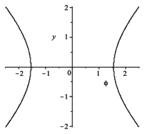
(a)

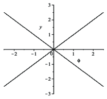
(b)

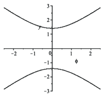
(c)

Figure 1: The phase portraits of system (2.5)($c=\gamma$). (a) $g<0$; (b) $g=0$; (c) $g>0$.

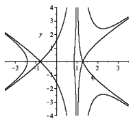
(a)

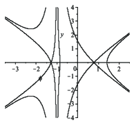
(b)

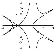
(c)

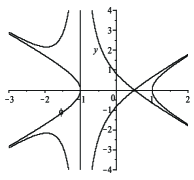
(d)

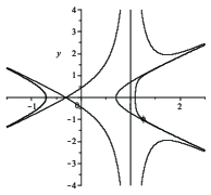
(e)

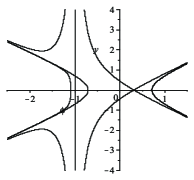
(f)

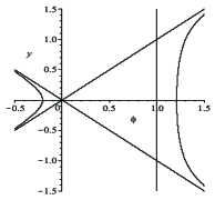
(g)

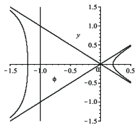
(h)

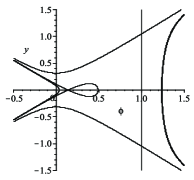
(i)

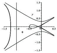
(j)

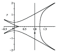
(k)

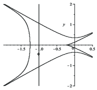
(l)

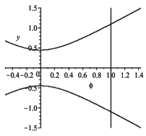
(m)

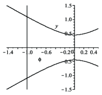
(n)

Figure 2: The phase portraits of system (2.5) ($c\neq\gamma$). (a) $g<g_{2}(c),c>\gamma$; (b) $g<g_{2}(c),c<\gamma$; (c) $g=g_{2}(c),c>\gamma$; (d)$g=g_{2}(c),c<\gamma$; (e) $g_{2}(c)<g<0,c>\gamma$; (f) $g_{2}(c)<g<0,c<\gamma$; (g) $g=0,c>\gamma$; (h) $g=0,c<\gamma$; (i) $0<g<g_{1}(c),c>\gamma$; (j)$0<g<g_{1}(c),c<\gamma$; (k) $g=g_{1}(c),c>\gamma$; (l) $g=g_{1}(c),c<\gamma$;(m)$g>g_{1}(c),c>\gamma$;(n)$g>g_{1}(c),c<\gamma$.

3 Solitons, peakons and periodic cusp wave solutions

Theorem 3.1

Given arbitrary constant $c\neq\gamma$, let $\xi=x-ct$, then

(1) when $0<g<g_{1}(c)$,

(i) if $c>\gamma$, then Eq.(1.3) has the following smooth hump-like soliton solutions

$$\beta_{1}(\varphi_{1}^{+})=\beta_{1}(\varphi)e^{-|\xi|}\quad for\quad\varphi_{0}^{-}<\varphi<\varphi_{1}^{+},$$ (3.1)

(ii) if $c<\gamma$, then Eq.(1.3) has the following smooth valley-like soliton solutions

$$\beta_{2}(\varphi)=\beta_{2}(\varphi_{1}^{-})e^{-|\xi|}\quad for\quad\varphi_{1}^{-}<\varphi<\varphi_{0}^{+},$$ (3.2)

(2) when $g=0$ʱ, Eq.(1.3) has the following peaked soliton solutions

$$\varphi=(c-\gamma)e^{-|\xi|},$$ (3.3)

(3) when $g_{2}(c)<g<0$,

(i) if $c>\gamma$, then Eq.(1.3) has the following periodic cusp wave solutions

$$u(x,t)=\varphi_{3}(x-ct-2nT)\quad for\quad(2n-1)T<x-ct<(2n+1)T,$$ (3.4)

(ii) if $c<\gamma$, then Eq.(1.3) has the following periodic cusp wave solutions

$$u(x,t)=\varphi_{4}(x-ct-2nT)\quad for\quad(2n-1)T<x-ct<(2n+1)T,$$ (3.5)

where

$$\beta_{1}(\varphi)=\frac{(2\sqrt{\varphi^{2}+l_{1}\varphi+l_{2}}+2\varphi+l_{1})(\varphi-\varphi_{0}^{-})^{\alpha_{1}}}{(2\sqrt{a_{1}}\sqrt{\varphi^{2}+l_{1}\varphi+l_{2}}+b_{1}\varphi+l_{3})^{\alpha_{1}}},$$ (3.6)

$$\beta_{2}(\varphi)=\frac{(2\sqrt{\varphi^{2}+m_{1}\varphi+m_{2}}+2\varphi+m_{1})(\varphi-\varphi_{0}^{+})^{\alpha_{2}}}{(2\sqrt{a_{2}}\sqrt{\varphi^{2}+m_{1}\varphi+m_{2}}+b_{2}\varphi+m_{3})^{\alpha_{2}}},$$ (3.7)

$$l_{1}=-\frac{3(c-\gamma)+\sqrt{(c-\gamma)^{2}-8g}}{2},$$ (3.8)

$$l_{2}=\frac{3(c-\gamma)^{2}-4g+5(c-\gamma)\sqrt{(c-\gamma)^{2}-8g}}{8},$$ (3.9)

$$l_{3}=\frac{(c-\gamma)^{2}-4g+3(c-\gamma)\sqrt{(c-\gamma)^{2}-8g}}{2},$$ (3.10)

$$m_{1}=-\frac{3(c-\gamma)-\sqrt{(c-\gamma)^{2}-8g})}{2},$$ (3.11)

$$m_{2}=\frac{3(c-\gamma)^{2}-4g-5(c-\gamma)\sqrt{(c-\gamma)^{2}-8g}}{8},$$ (3.12)

$$m_{3}=\frac{(c-\gamma)^{2}-4g-3(c-\gamma)\sqrt{(c-\gamma)^{2}-8g}}{2},$$ (3.13)

$$a_{1}=\frac{((c-\gamma)^{2}-8g+3(c-\gamma)\sqrt{(c-\gamma)^{2}-8g}}{4},$$ (3.14)

$$a_{2}=\frac{((c-\gamma)^{2}-8g-3(c-\gamma)\sqrt{(c-\gamma)^{2}-8g}}{4},$$ (3.15)

$$b_{1}=-(c-\gamma)-\sqrt{(c-\gamma)^{2}-8g},$$ (3.16)

$$b_{2}=-(c-\gamma)+\sqrt{(c-\gamma)^{2}-8g},$$ (3.17)

$$\alpha_{1}=-\frac{3(c-\gamma)+\sqrt{(c-\gamma)^{2}-8g}}{2\sqrt{(c-\gamma)^{2}-8g+3(c-\gamma)\sqrt{(c-\gamma)^{2}-8g}}},$$ (3.18)

$$\alpha_{2}=\frac{-3(c-\gamma)+\sqrt{(c-\gamma)^{2}-8g}}{2\sqrt{(c-\gamma)^{2}-8g-3(c-\gamma)\sqrt{(c-\gamma)^{2}-8g}}},$$ (3.19)

$$\varphi_{3}(\xi)=l_{+}e^{-|\xi|}+l_{-}e^{|\xi|}\quad for\quad\sqrt{-g}\leq\varphi_{3}\leq c-\gamma,$$ (3.20)

$$\varphi_{4}(\xi)=l_{+}e^{|\xi|}+l_{-}e^{-|\xi|}\quad for\quad c-\gamma\leq\varphi_{4}\leq-\sqrt{-g},$$ (3.21)

$$l_{\pm}=\frac{c-\gamma\pm\sqrt{(c-\gamma)^{2}+g}}{2},$$ (3.22)

$$T=\left|\ln(\sqrt{-g}+\sqrt{-2g})-\ln(2l_{-})\right|.$$ (3.23)

$$\varphi_{1}^{\pm}=\frac{3}{4}(c-\gamma)\pm\frac{1}{4}\sqrt{(c-\gamma)^{2}-8g}\mp\frac{1}{2}\sqrt{(c-\gamma)^{2}\mp(c-\gamma)\sqrt{(c-\gamma)^{2}-8g}},$$ (3.24)

$\varphi_{0}^{+}$ and $\varphi_{0}^{-}$ are as in (2.11).

Before proving this theorem, we take a set of data and employ Maple to display the graphs of smooth solion, peaked soliton and periodic cuspon solutions of Eq.(1.3), see Fig.3-Fig.7.

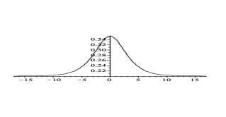
(a)

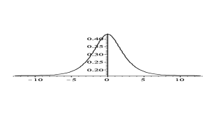
(b)

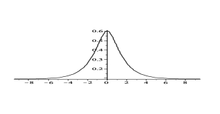
(c)

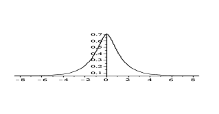
(d)

Figure 3: Smooth hump-like soliton solutions of Eq.(1.3)( $c=2$, $\gamma=1$). (a) $g=0.12$; (b)g=0.1; (c) g=0.075; (d) g=0.05.

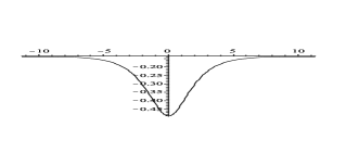
(a)

(b)

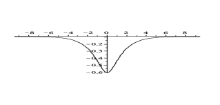
(c)

(d)

Figure 4: Smooth valley-like soliton solutions of Eq.(1.3).($c=1$, $\gamma=2$). (a) g = 0.12; (b) g=0.1; (c) g=0.075; (d) g=0.05.

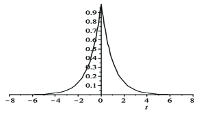
(a)

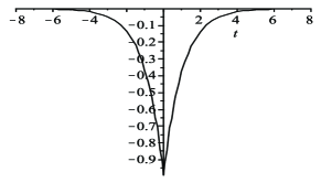
(b)

Figure 5: Peaked soliton solutions of Eq.(1.3). (a) $c=2$, $\gamma=1$; (b) $c=1$, $\gamma=2$.

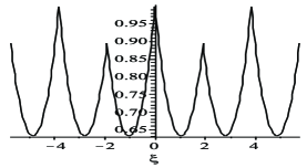
(a)

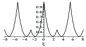
(b)

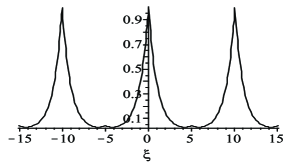
(c)

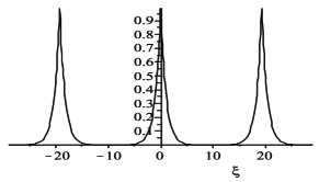
(d)

Figure 6: Period cuspon solutions of Eq.(1.3)( $c=2$, $\gamma=1$). (a) g = -0.4; (b) g=-0.1; (c) g=-0.01; (d) g=-0.0000001.

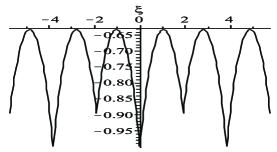
(a)

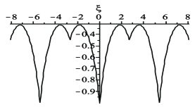
(b)

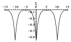
(c)

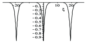
(d)

Figure 7: Period cuspon solutions of Eq.(1.3)($c=1$, $\gamma=2$). (a) g = -0.4; (b) g=-0.1; (c) g=-0.01; (d) g=-0.0000001.

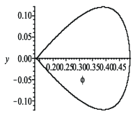
(a)

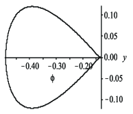
(b)

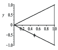
(c)

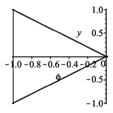
(d)

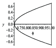
(e)

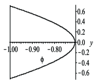
(f)

Figure 8: The orbits of system (2.5) connecting with the saddle points. (a)$0<g<g_{1}(c),c>\gamma$; (b) $0<g<g_{1}(c),c<\gamma$; (c) $g=0,c>\gamma$; (d) $g=0,c<\gamma$; (e) $g_{2}(c)<g<0,c>\gamma$; (f) $g_{2}(c)<g<0,c<\gamma$.

Proof. Usually, a solion solution of Eq.(1.3) corresponds to a homoclinic orbit of system (2.5) and a periodic travelling wave solution of Eq.(1.3) corresponds to a periodic orbit of system (2.5). The graphs of homoclinic orbit, periodic orbit of system (2.5) and their limit curves are shown in Fig.8.

(1) When $0<g<g_{1}(c),c>\gamma$, system (2.5) has a homoclinic orbit (see Fig.8(a)). This homoclinic orbit can be expressed as

$$y=\pm\frac{(\varphi-\varphi_{0}^{-})\sqrt{\varphi^{2}+l_{1}\varphi+l_{2}}}{c-\gamma-\varphi}\quad for\quad\varphi_{0}^{-}<\varphi<\varphi_{1}^{+}.$$ (3.25)

Substituting (3.25) into the first equation of system (2.3) and integrating along this homoclinic orbit, we obtain (3.1).

When $0<g<g_{1}(c),c<\gamma$, we can obtain (3.2) in similar way.

(2) When $g=0,c>\gamma$, system (2.5) has a homoclinic orbit that consists of the following three line segments (see Fig.8(c)).

$$y=\pm\varphi\quad for\quad\varphi_{0}^{-}\leq\varphi\leq\varphi_{1}^{+},$$ (3.26)

and

$$\varphi=c-\gamma\quad for\quad-\sqrt{(c-\gamma)^{2}+g}\leq y\leq\sqrt{(c-\gamma)^{2}+g}.$$ (3.27)

Substituting (3.26) into the first equation of system (2.3) and integrating along this orbit, we obtain (3.3).

When $g=0,c<\gamma$, we can also obtain (3.3).

(3) When $g_{2}(c)<g<0,c>\gamma$, system (2.5) has a periodic orbit (see Fig. 8(e)). This periodic orbit can be expressed as

$$y=\pm\sqrt{\varphi^{2}+g}\quad for\quad\sqrt{-g}\leq\varphi\leq c-\gamma,$$ (3.28)

and

$$\varphi=c-\gamma\quad for\quad-\sqrt{(c-\gamma)^{2}+g}\leq y\leq\sqrt{(c-\gamma)^{2}+g}.$$ (3.29)

Substituting (3.28) into the first equation of system (2.3) and integrating along this periodic orbit, we obtain (3.4).

When $g_{2}(c)<g<0,c<\gamma$, we can obtain (3.5).  

Remark 3.1

From the above discussion, we can see that when $g<0,g\rightarrow 0$, the period of the periodic cusp wave solution becomes bigger and bigger, and the periodic cuspon solutions (3.4) and (3.5) tend to the peaked soliton solutions (3.3) . When $g>0,g\rightarrow 0$, the smooth hump-like soliton solutions (3.1) and the smooth valley-like soliton solutions (3.2) lose their smoothness and tend to the peaked soliton solutions (3.3).

4 Discussion

In this paper, we obtain the solitons, peakons, and periodic cuspons of a generalized Degasperis-Procesi equation (1.3). These solitons denote the nonlinear localized waves on the shallow water’s free surface that retain their individuality under interaction and eventually travel with their original shapes and speeds. The balance between the nonlinear steepening and dispersion effect under Eq.(1.3) gives rise to these solitons.

The peakon travels with speed equal to its peak amplitude. This solution is nonanalytic, having a jump in derivative at its peak. Peakons are true solitons that interact via elastic collisions under Eq.(1.3). We claim that the existence of a singular straight line for the planar dynamical system (2.3) is the original reason why the travelling waves lose their smoothness.

Also, the periodic cuspon solution is nonanalytic, having a jump in derivative at its each cusp.

References

- [1] A. Degasperis, M. Procesi, Asymptotic integrability, in: A. Degasperis, G. Gaeta (Eds.), Symmetry and Perturbation Theory (SPT 98), Rome, December 1998, World Scientific, River Edge, NJ, 1999, 23-37.
- [2] A. Degasperis, D. D. Holm, A. N. W. Hone, A new integral equation with peakon solutions, Theo. Math. Phys. 133 (2002) 1463-1474.
- [3] Z. Y. Yin, On the cauchy problem for an integrable equation with peakon solutions, I11. J. Math. 47 (2003) 649-666.
- [4] Z. Y. Yin, Global weak solutions to a new periodic integrable equation with peakon solutions, J. Funct. Anal. 212 (2004) 182-194.
- [5] Z. Y. Yin, Global solutions to a new integrable equation with peakons, Ind. Univ. Math. J. 53 (2004) 1189-1210.
- [6] Z. Y. Yin, Global existence for a new periodic integrable equation, J. Math. Anal. Appl. 283 (2003) 129-139.
- [7] Y. Zhou, Blow-up phenomena for the integrable Degasperis-Procesi equation, Phys. Lett. A. 328 (2004) 157-162.
- [8] J. Escher, Y. Liu, Z. Y. Yin, Global weak solutions and blow-up structure for the Degasperis-Procesi equation, J. Funct. Anal. 241 (2006) 57-485.
- [9] Z. Y. Yin, Well-posedness, blow up, and global existence for an integrable shallow water equation, Disc. Conti. Dyn. Sys. 11 (2004) 393-411.
- [10] Y. Liu, Z. Y. Yin, Global existence and blow-up phenomena for the Degasperis-Procesi equation, Commun. Math. Phys. 267 (2006) 801-820.
- [11] V. O. Vakhnenko, E. J. Parkes, Periodic and solitary-wave solutions of the Degasperis-Procesi equation, Chaos Solitons and Fractals 20 (2004) 1059-1073.
- [12] Y. Matsuno, Multisoliton solutions of the Degasperis-Procesi equation and their peakon limit, Inverse Problems 21 (2005) 1553-1570.
- [13] Y. Matsuno, Cusp and loop soliton solutions of short-wave models, for the Camassa-Holm and Degasperis-Procesi equations, Phys. Lett. A 359 (2006) 451-457.
- [14] H. Lundmark, J. Szmigielski, Multi-peakon solutions of the Degasperis-Procesi equation, Inverse Problems 19 (2003) 1241-1245.
- [15] J. Lenells, Traveling wave solutions of the Degasperis-Procesi equation, J. Math. Anal. Appl. 306 (2005) 72-82.
- [16] H. Lundmark, Formation and dynamics of shock waves in the Degasperis-Procesi equation, J. Nonlinear Sci. 17 (2007) 169-198.
- [17] J. Escher, Y. Liu, Z. Y. Yin, Shock waves and blow-up phenomena for the periodic degasperis equation, Ind. Univ. Math. J. 56 (2007) 187-117.
- [18] L. Q. Yu, L. X. Tian, X. D. Wang, The bifurcation and peakon for Degasperis-Procesi equation, Chaos, Solitons and Fractals 30 (2006) 956-966.
- [19] D. Luo, et al., Bifurcation Theory and Methods of Dynamical Systems, World Scientific Publishing Co., London, 1997.