Vibrational interference of Raman and high-harmonic generation pathways

Abstract

Experiments have shown that the internal vibrational state of a molecule can affect the intensity of high harmonic light generated from that molecule. This paper presents a model which explains this modulation in terms of interference between different vibrational states occurring during the high harmonic process. In addition, a semiclassical model of the continuum electron propagation is developed which connects with rigorous treatments of the electron-ion scattering.

I Introduction

In the usual three step model of high harmonic generation, HHG is treated as a purely electronic process. A single active electron tunnels free of a parent molecule and eventually scatters from it, but the molecule itself is treated in essentially the same way as a lone atom; no more than a complicated potential influencing the active electron. However, molecules differ from atoms in an essential way because they possess non electronic internal degrees of freedom, which can themselves be affected by the high harmonic process.

The possibility that such internal degrees of freedom could play a detectable role in HHG is intriguing, because the intrinsic timescale in HHG – the time necessary to ionize, propagate and rescatter – is only half a laser cycle. This is faster than many chemically interesting processes, holding out the possibility that HHG could serve as a probe of molecular motion. Alternatively, tailoring the state of a molecule prior to HHG could serve to give additional control over the generated light.

These issues were brought to the fore by an experiment at JILA Wagner et al. (2006). In the experiment, a high harmonic generating laser pulse was preceded by a weaker pulse whose effect was to stimulate Raman-active vibrations in SF₆ molecules. Varying the delay between the two pulses was observed to modulate the intensity of the HHG light generated by the second pulse. Moreover, the modulation corresponds to the frequencies of the Raman-active normal modes stimulated by the first pulse. None of the 3 non-Raman-active vibrational modes of SF₆ were detected in the modulated signal.

This paper presents a quantum mechanical model of high harmonic generation in molecules. This model provides a framework to interpret the observed modulation of high harmonic intensities observed in the JILA experiment, and is easily extended to systems with more complicated dynamics. Secondly, it presents a version of the three step model which has been improved for the purpose of treating HHG in molecules with relevant internal degrees of freedom. Finally, the modulations predicted by this improved model are compared with the modulations observed in the JILA experiment. This paper recapitulates and extends work which originally appeared in Walters et al. (2007).

II The Vibrational Wavefunction of the Molecule

An important difference between atomic and molecular systems, probed by the aforementioned experimentWagner et al. (2006) is the presence of vibrational degrees of freedom in the latter. For an $M$-atom molecule, this corresponds to $N=3M-6$ ($N=3M-5$ for linear molecules) internal degrees of freedom, which can be expressed in normal mode coordinates. The vibrational wavefunction of the molecule can then be expanded as the product of simple harmonic oscillator basis functions in each of the normal modes of the molecule:

$$\ket{\psi_{\text{vib}}}=\sum_{n_{1},n_{2},\ldots n_{N}=0}^{\infty}A_{n_{1},n_{2},\ldots,n_{N}}\ket{n_{1},n_{2},\ldots n_{N}}$$ (1)

where

$$\bf{a^{(i){\dagger}}}\bf{a^{(i)}}\ket{n_{1}\ldots n_{N}}=n_{i}\ket{n_{1}\ldots n_{N}}$$ (2)

where $\ket{n_{1}n_{2}\ldots n_{N}}$ is the outer product of simple harmonic oscillator state $\ket{n_{1}}$ in the first normal mode, $\ket{n_{2}}$ in the second normal mode, and so on.

For the purposes of this paper, all operators will be expanded to first order in raising $\bf{a^{{\dagger}(i)}}$ and lowering $\bf{a^{(i)}}$ operators in each normal mode $i$. At this level of approximation, the evolution of the vibrational wavefunction becomes separable, and the overall coefficient $A_{n_{1}n_{2}\ldots n_{N}}(t)$ can be factored into the product of individual coefficients $a_{n_{i}}(t)$:

$$A_{n_{1}n_{2}\ldots n_{N}}(t)=a_{n_{1}}(t)a_{n_{2}}(t)\ldots a_{n_{N}}(t).$$ (3)

(Note that the coefficients $a_{n_{i}}(t)$ should not be confused with lowering operators $\bf{a^{(i)}}$.)

In the interests of simplicity and clarity, the remainder of this paper will use a 1-D picture, describing the evolution of the vibrational wavefunction for each single normal mode. The concepts from the 1-D model extend readily to the higher intensity regime of coupled modes, in the event that operators involving two or more raising or lowering operators become important.

III Vibrational Interference

Although high harmonic generation is primarily an electronic process, the vibrational state of the molecule can affect the harmonic intensity. This occurs because at several points in the high harmonic process, the vibrational wavefunction has amplitudes either to stay unchanged or to “hop” up or down from simple harmonic oscillator state $\ket{n}$ to states $\ket{n\pm 1}$, much in the same way that a photon in a beamsplitter has amplitudes to take two or more paths. As in a beamsplitter experiment, two or more indistinguishable pathways interfere with one another and modulate the output signal detectably. The multiple pathways at play in the high harmonic process are diagrammed in Figure 1.

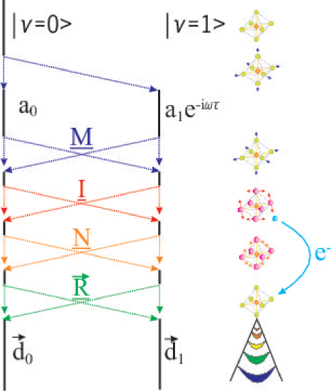
Figure 1: The vibrational interference model Walters et al. (2007) in one dimension. The molecule ends the first (Raman) pulse in a superposition of the $\nu=0$ and $\nu=1$ vibrational states. After a time delay, the two vibrational states are mixed by stimulated Raman scattering (transfer matrix M), “hopping” during ionization (I) and recombination (R), as well as evolution of the ionic wavefunction while the electron is away (N). Interference between adjacent vibrational states modulates the high harmonic signal.

Raman Excitation

The first opportunity to change vibrational states occurs when the vibrationally cold molecules are subjected to the weak, off-resonant initial pulse. This causes the molecule to undergo stimulated Raman scattering. At the start of the first pulse the molecule is in the $\ket{0}$ vibrational state, and it is then driven into a coherent superposition of the zeroth and first vibrational states

$$\ket{\psi_{\text{vib}}}=a_{0}(0)\ket{0}+a_{1}(0)\ket{1}$$ (4)

by the end of the pulse. (For the pulse length and intensity used in the JILA experiment, calculations show no appreciable population of the $\ket{2}$ or higher states after the Raman pulse. Accordingly, the $\ket{2}$ and higher states have been dropped from this analysis.) Because only one normal mode is used in this analysis, the $N$ quantum number has been dropped, so that $a_{0}=a_{1_{0}}(0)$ and $a_{1}=a_{1_{1}}(0)$. $t=0$ is chosen at some time after the end of the first pulse, when the stimulated Raman scattering is over.

The vibrational state coefficients follow equations of motion given by

$$\begin{split}i\dot{a}_{n_{i}}(t)=\omega_{i}\left(n_{i}+\frac{1}{2}\right)a_{n_{i}}(t)-\frac{1}{2}\sum_{A,B}E_{A}(t)E_{B}(t)\times\\ \left[\alpha_{AB}a_{n_{i}}+\partial_{i}\alpha_{AB}(\sqrt{n_{i}+1}a_{n_{i}+1}+\sqrt{n_{i}}a_{n_{i}-1})\right].\end{split}$$ (5)

Here $\omega_{i}$ is the normal mode frequency, indices $A$ and $B$ run over $\{x,y,z\}$, $E_{A}(t)$ is the component of the electric field in the (body-frame) $A$ direction at time $t$, $Q_{i}$ is the normalized displacement associated with normal mode $i$ and $\alpha_{AB}(Q_{1},Q_{2},...)$ is the polarizability tensor of the molecule. These equations of motion have off-diagonal elements only if $\partial_{i}\alpha_{AB}\equiv\left(2m\omega_{i}\right)^{-1/2}\partial\alpha_{AB}/\partial Q_{i}|_{Q_{i}=0}\neq 0$, which is the condition for a mode to be Raman active. The polarizability tensor and its derivatives are found by performing an unrestricted Hartree-Fock calculation Frisch et al. (1998) using the aug-cc-pVTZ basis set. Dunning Jr (1989)

Between the two pulses, the $\ket{0}$ and $\ket{1}$ states evolve as eigenstates of the simple harmonic oscillator Hamiltonian. The states are then mixed once again by stimulated Raman scattering during the high harmonic generating pulse. These effects are approximated by a unitary $2\times 2$ transfer matrix $\underline{M}$, where $M_{ij}$ is the amplitude to be in state $\ket{i}$ at the instant of ionization after beginning the second pulse in state $\ket{j}$.

Ionization and Recombination

The vibrational wavefunction evolves further during each of the three steps –ionization, propagation, and recombination–of the three step model. The molecule’s vibrational state hops up or down a level during ionization, evolves while the propagating electron is away from the molecule, and hops once again when the electron recombines with the parent ion.

These hopping amplitudes arise because ionization and recombination, commonly thought of as purely electronic processes, are both strongly modulated by molecular distortions. This is the simplest way in which the internal degrees of freedom in molecules allows for behavior that has no analogue in atomic systems. Nonzero derivatives of ionization and recombination amplitudes translate directly into amplitudes for the molecule to change its vibrational state during these processes. Taylor-expanding the ionization operator about the equilibrium configuration of the neutral molecule,

$$\hat{I}=\hat{I}|_{\text{eq}}+\frac{\partial\hat{I}}{\partial Q}Q+\mathbb{O}(Q^{2}),$$ (6)

using the identity $Q=(\bf{a}+\bf{a^{{\dagger}}})/\sqrt{2m\omega}$ and substituting $I_{0}=\hat{i}|_{\text{eq}}$, $I_{1}=(2m\omega)^{-1/2}\frac{\partial\hat{I}}{\partial Q}$, the ionization operator can be rewritten

$$\hat{I}=I_{0}+I_{1}(\bf{a}+\bf{a^{{\dagger}}}).$$ (7)

Identical logic gives the recombination dipole vector operator

$$\hat{\vec{R}}=\vec{R}_{0}+\vec{R}_{1}(\bf{a}+\bf{a^{{\dagger}}})$$ (8)

Vibrational Dynamics of the Parent Ion

Between the times of ionization and recombination, the evolution of the internal state of SF${}_{6}^{+}$ is quite complicated. This is because SF₆ has three degenerate orbitals at the point of maximum symmetry. Thus, at any nuclear configuration near this maximum symmetry point, these three SF${}_{6}^{+}$ orbitals are very nearly degenerate, and are mixed with one another strongly by molecular distortions. Orbital degeneracies can be broken and orbital energies can cross even with relatively small distortions. Because of this, it is necessary to treat this interplay between electronic and vibrational states when describing the dynamics of SF${}_{6}^{+}$ in the vicinity of the maximum symmetry point.

In its maximum symmetry configuration, SF${}_{6}^{+}$ belongs to the O_h point group, with three degenerate T_1g orbitals which transform like axial vectors $\hat{x}$, $\hat{y}$ and $\hat{z}$. When the molecule is distorted away from the maximum symmetry point via either an E_g or a T_2g distortion, the triple degeneracy breaks up into three nondegenerate electronic orbitals. The fully symmetric A_1g or “breathing” mode preserves the triple degeneracy.

The full vibronic (vibrational-electronic) Jahn-Teller coupling matrix for a triply degenerate system is given byEstreicher and Estle (1985); Moffitt and Thorson (1957); Bersuker and Borisovich (1984)

$$H_{T}=\begin{pmatrix}g_{1}-g_{\theta}+\sqrt{3}g_{\epsilon}&g_{\zeta}&g_{\eta}\\ g_{\zeta}&g_{1}-g_{\theta}-\sqrt{3}g_{\epsilon}&g_{\xi}\\ g_{\eta}&g_{\xi}&g_{1}+2g_{\theta}\end{pmatrix}$$ (9)

This matrix represents the coupling between the states with $\hat{x}$, $\hat{y}$, and $\hat{z}$ symmetry, caused by vibrational operators, so that $g_{\zeta}$ represents the off-diagonal coupling between the states with $\hat{x}$ and $\hat{y}$ symmetry, $g_{\eta}$ the off-diagonal coupling between the states with $\hat{x}$ and $\hat{z}$ symmetry, and $g_{\xi}$ represents the off-diagonal coupling between the states with $\hat{y}$ and $\hat{z}$ symmetry.

Defining the E_g normal mode coordinates $Q_{\theta}$ and $Q_{\epsilon}$, which transform like $2z^{2}-x^{2}-y^{2}$ and $x^{2}-y^{2}$ respectively, and the T_2g normal mode coordinates $Q_{\xi}$, $Q_{\eta}$ and $Q_{\zeta}$ respectively as the coordinates that transform like $yz$,$xz$, and $xy$, the functions $g_{i}$ are given by Estreicher and Estle (1985)

$$g_{1}= \frac{1}{2}K_{E}(Q_{\theta}^{2}+Q_{\epsilon}^{2})+\frac{1}{2}K_{T}(Q_{\xi}^{2}+Q_{\eta}^{2}+Q_{\zeta}^{2})$$ (10)

$$g_{\theta}= \frac{1}{\sqrt{3}}V_{E_{g}}Q_{\theta}+N_{E}(Q_{\epsilon}^{2}-Q_{\theta}^{2})+N_{1}(2Q_{\zeta}^{2}-Q_{\xi}^{2}-Q_{\eta}^{2})$$ (11)

$$g_{\epsilon}= \frac{1}{\sqrt{3}}V_{E_{g}}Q_{\epsilon}+2N_{E}Q_{\theta}Q_{\epsilon}+\sqrt{3}N_{1}(Q_{\xi}^{2}-Q_{\eta}^{2})$$ (12)

$$g_{\xi}= V_{T_{2g}}Q_{\xi}+N_{T}Q_{\eta}Q_{\zeta}+N_{2}Q_{\xi}(\sqrt{3}Q_{\epsilon}-Q_{\theta})$$ (13)

$$g_{\eta}= V_{T_{2g}}Q_{\eta}+N_{T}Q_{\zeta}Q_{\xi}+N_{2}Q_{\eta}(-\sqrt{3}Q_{\epsilon}-Q_{\theta})$$ (14)

$$g_{\zeta}= V_{T_{2g}}Q_{\zeta}+N_{T}Q_{\xi}Q_{\eta}+2N_{2}Q_{\zeta}Q_{\theta}$$ (15)

These constants were found by performing a CASSCF state-averaged calculation for the three lowest energy states of SF${}_{6}^{+}$ for various displacements of the molecule away from the maximum symmetry configuration. These energies are shown in Figure 2. The CASSCF calculations were carried using a basis of Hartree-Fock orbitals calculated for neutral SF₆. These three adiabatic energies were then fitted to the eigenvalues of the diabatic Jahn-Teller coupling matrix. This process yielded $V_{T_{2g}}$=.001209 H/bohr, $V_{E_{g}}$=.1406 H/bohr, $N_{1}$=-.0362 H/bohr², $K_{T_{2g}}$=.7288 H/bohr², $K_{E_{g}}$=1.8486 H/bohr². For the A_1g mode, which does not enter into the vibronic Hamiltonian, an adiabatic potential $E=V_{A_{1g}}Q_{A_{1g}}+\frac{1}{2}K_{A_{1g}}Q_{A_{1g}}^{2}$, with $V_{A_{1g}}$=.0645 H/bohr, $K_{A_{1g}}$=2.98 H/bohr² gives the potential energy surface for all three electronic states.

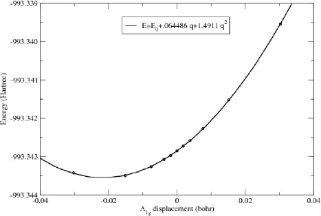
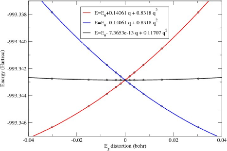
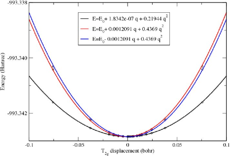
Figure 2: a)Spherically symmetric $A_{1g}$ (breathing mode) distortions change electronic state energies, but preserve the triple degeneracy. Non symmetric E_g (b) and T_2g (c) distortions break the triple degeneracy of SF${}_{6}^{+}$ at the maximum symmetry point. Adiabatic energies are fitted to the eigenvalues of the vibronic coupling matrix (equation 9) to solve for the vibronic coupling constants.

Here there is a significant distinction between distortions of type $E_{g}$, which break the triple degeneracy but have no linear off-diagonal terms, and distortions of type T_2g, which do contribute to off-diagonal coupling. For small distortions, an adiabatic electronic state of an E_g distorted molecule will have the same symmetry – $\hat{x}$, $\hat{y}$, $\hat{z}$ – as the diabatic electronic states. The adiabatic electronic states of a T_2g-distorted molecule, on the other hand, are linear combinations of the diabatic orbitals. An important simplification is that $V_{T_{2g}}$, controlling off-diagonal coupling between different electronic states, is small in SF${}_{6}^{+}$ and can be neglected for the short time between ionization and recombination.

The evolution of the ionic wavefunction is calculated in the vibrational basis of the neutral molecule, but using potential energy surfaces calculated for the ion. Potential energy curves are found to quadratic order in $Q$ using quantum chemistry calculations, then expressed in terms of raising and lowering operators by substituting $Q=(2m\omega)^{-1/2}(\bf{a}+\bf{a^{{\dagger}}})$, $Q^{2}=(2m\omega)^{-1}(\bf{a}+\bf{a^{{\dagger}}})(\bf{a}+\bf{a^{{\dagger}}})$. All terms up to linear in raising and lowering operators are then used to integrate the time-dependent Schrödinger equation to find a transfer matrix $\underline{N}$ describing the evolution of the ionic wavefunction between ionization and recombination.

Modulation of Harmonic Intensity

In the two-state model used here, the $i-$th vibrational wavefunction of the neutral molecule after recombination has occurred is $\ket{\psi_{\text{vib}}}=d_{0}\ket{0}+d_{1}\ket{1}$, where

$$\begin{pmatrix}\vec{d}_{0}&\vec{d}_{1}\end{pmatrix}=\begin{pmatrix}a_{0}(0)&a_{1}(0)e^{-i\omega\tau}\end{pmatrix}\underline{M}^{T}\underline{I}^{T}\underline{N}^{T}\underline{\vec{R}}^{T}.$$ (16)

Here, e.g. $\underline{M}^{T}$ denotes the transpose of matrix $\underline{M}$.

The number of photons emitted in a given harmonic is proportional to $\vec{d}_{0}\cdot\vec{d}^{*}_{0}+\vec{d}_{1}\cdot{\vec{d}^{*}_{1}}$. The high harmonic intensity is a sum over all Raman active modes $i$:

$$P(\tau)=P_{0}+\Sigma_{i}P_{1}^{(i)}\cos\left(\omega_{i}\tau+\delta_{i}\right)$$ (17)

. The static $P_{0}$ primarily results from terms of the form $a_{0}(0)^{*}a_{0}(0)$, while $P_{1}$ results from terms of the form $a_{0}(0)a_{1}(0)^{*}e^{i\omega\tau}$ and $a_{1}(0)a_{0}(0)^{*}e^{-i\omega\tau}$. Defining $\underline{W}=\underline{M}^{{\dagger}}\underline{I}^{{\dagger}}\underline{N}^{{\dagger}}\underline{\vec{R}}^{{\dagger}}\cdot\underline{\vec{R}NIM}$, $P_{0}=a_{0}(0)^{*}W_{00}a_{0}(0)$ and $P_{1}\cos\left(\omega t+\delta\right)=\frac{1}{2}(a_{1}^{*}e^{i\omega\tau}W_{10}a_{0}(0)+\text{c.c.})$. Since $I_{1}$ and $R_{1}$ are small relative to $I_{0}$ and $R_{0}$, only their first-order terms are kept.

IV Describing the Continuum Electron

The evolution of the continuum electron wavefunction is strongly influenced by interactions with both the parent ion and the driving laser. When the electron first tunnels free out of the parent molecule, its wavefunction is determined by both the molecular potential and the electric field of the laser. Once free, it propagates in the time-varying field of the laser while feeling a weak force due to Coulomb attraction to the parent ion. Finally it recollides with the parent ion, and is once again strongly distorted by the molecular potential.

A full solution of the time dependent Schrödinger equation for this process would be computationally demanding for complicated molecules such as SF₆. In addition, much of the information in the continuum wavefunction is not relevant to the HHG problem: only a small part of the wavefunction overlaps with the unoccupied orbital into which the rescattering electron recombines.

One frequently used treatment which avoids the complications of the full time-dependent Schrödinger equation Corkum (1993); Lewenstein et al. (1994a) is based on a classical or semiclassical propagation of the continuum electron, ignoring the ionic Coulomb potential. The returning electron wavefunction is the approximated as a plane wave throughout the recombination process. This approach has been successful in describing the high harmonic cutoff, the chirp of the emitted high harmonic light and other quantities of interest in atomic systemsLewenstein et al. (1994b); Kazamias and Balcou (2004). However, as was shown in Walters et al. (2008), the plane wave approximation is not adequate to describe the returning electron because of the tremendous distortion caused by the electron’s interaction with the ionic potential and by exchange effects with the other electrons in the molecule.Le et al. (2008); Smirnova et al. (2008) For the time-reversed problem of photoionization, it is known that the plane wave approximation is prone to error for photoelectron energies smaller than the deepest K-shell binding energy. Energies attained in high harmonic generation experiments usually fall below this range.

This section gives a semiclassical model of the free electron propagation which improves upon the Corkum/Lewenstein model by connecting with calculated short-range wavefunctions. Any method could be used to calculate these short-range wavefunctions. In this treatment, the tunneling wavefunction is modeled semiclassically using ideas based on the initial value representation Miller (2001); Nakamura (2005). The continuum wavepacket of the recolliding electron is described in terms of electron-molecule scattering states as used in Walters et al. (2008), calculated in the absence of an external electric field.

In this way, the molecular potential nontrivially affects the electron wavefunction at the two times when the electron is near the molecular ion. When the electron is far from the molecule, the comparatively simple evolution of its wavefunction is described using the shortest-time, dominant contribution to the Gutzwiller propagator Gutzwiller (1990). Finally, stationary phase arguments serve to identify the isolated trajectories that encapsulate the effect of the electron propagation in the field on high harmonic generation, greatly reducing the computational burden of propagating the continuum electron wavefunction.

IV.1 Tunneling Ionization

During the ionization step, the tunneling electron wavefunction is described in a simple 1-D WKB tunneling picture, in which electrons are allowed to tunnel only in directions parallel to the laser’s applied electric field. This approach is motivated by the semiclassical “initial value representation” Miller (2001); Nakamura (2005), where a source wavefunction acquires an imaginary phase (and hence an exponential growth or decay) along a trajectory that passes through a classically forbidden region. The unperturbed highest occupied molecular orbital (HOMO) here serves as the source wavefunction, so that the tunneling wavefunction is approximated by the unperturbed HOMO in the classically-allowed region near the molecule, connecting to a WKB exponential which is set equal to the HOMO at the inner turning point and decays exponentially until it reaches the outer turning point. SF₆ has three degenerate HOMOs: one of these is illustrated in Figure 3.

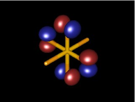
Figure 3: One of three degenerate orbitals of SF₆. Red denotes positive lobes; blue denotes negative lobes.

The classically forbidden region, illustrated in Figure 4, is defined by two turning points, $a$ and $b$, between which $V(x)-E>0$. The slope of $V(x)$ is $C_{1}$ at inner turning point $a$ and $C_{2}$ at outer turning point $b$. The tunneling wavefunction $\psi_{t}(\vec{r},t)$ is now found by applying WKB connection formulas. The appendix derives the ratio of the tunneling wavefunction at the outer turning point to the tunneling wavefunction at the inner turning point

$$\frac{\psi(x=b)}{\psi(x=a)}=\frac{1}{2}e^{-\Gamma}|\frac{C_{1}}{C_{2}}|^{1/6}\frac{\text{Bi}(0)}{\text{Ai}(0)}$$ (18)

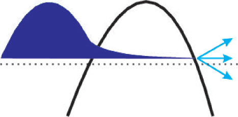
Figure 4: The tunneling wavefunction is approximated as an unperturbed molecular HOMO inside the classically allowed region, connecting to a decreasing WKB exponential in the classically forbidden region. Stationary phase trajectories leave from the outer turning point, beginning with zero velocity at time of ionization.

In this approximation, the tunneling wavefunction behaves like an Airy $Bi$ function near the outer turning point, i.e. it has no linear complex phase term. This property will be revisited in the section dealing with stationary phase analysis.

IV.2 Semiclassical Propagation

When the active electron has tunneled free from the molecule, the evolution of its wavefunction is controlled by the oscillating electric field of the laser, plus a residual Coulomb attraction to the molecular ion. This relatively simple evolution continues until the electron returns to the molecule, when the complicated molecular potential again becomes significant. During this excursion, until it re-enters the non-Coulomb part of the potential, the continuum wavefunction can be approximated using Gutzwiller’s semiclassical propagatorGutzwiller (1990):

$$\begin{split}K(\vec{r},t;\vec{r}_{0},t_{0})=\sum_{\text{cl. traj.}}(2\pi i)^{-3/2}\sqrt{C(\vec{r},t;\vec{r}_{0},t_{0})}\times\\ \exp(iS(\vec{r},t;\vec{r}_{0},t_{0})-i\phi)\end{split}$$ (19)

Here $S(\vec{r},t;\vec{r}_{0},t_{0})$ is the action integral $S=\int L(q,\dot{q},t)dt$ calculated for a classical trajectory starting at $(\vec{r}_{0},t_{0})$ and ending at $(\vec{r},t)$, while $C(\vec{r},t;\vec{r}_{0},t_{0})=|\frac{-\partial^{2}S}{\partial r_{0,A}}\partial r_{B}|$, where $r_{A}$ is the A-component of the vector $\vec{r}$. $\phi$ is a phase factor equal to $\frac{\pi}{2}$ times the number of conjugate points crossed by the trajectoryGutzwiller (1990).

This propagator acts on the tunneling wavepacket $\psi_{t}$ to give a semiclassical continuum wavepacket

$$\psi_{c}(\vec{r},t)=\int d^{3}\vec{r}_{0}\int dt_{0}K(\vec{r},t;\vec{r}_{0},t_{0})\psi_{t}(\vec{r}_{0},t_{0}).$$ (20)

until the molecular potential asserts itself during the rescattering.

During the terminal portion of the scattering process, when the scattering wavefunction acquires its maximum dipole matrix element with the molecular HOMO into which it recombines, the electronic wavefunction is expanded into a truncated (but in principle complete) basis of field-free electron-molecule scattering orbitals, calculated using techniques described in references Tonzani and Greene (2005, 2006); Tonzani (2007). Beyond the range of the molecular potential, i.e. for $r>r_{0}$, the $(l,m)$-th independent scattering state is expressed as a partial wave expansion in terms of incoming and outgoing Coulomb radial functions $f^{\pm}_{El}(r)$ and the scattering S-matrix as

$$\begin{split}\psi_{E,lm}(\vec{r})=\frac{1}{i\sqrt{2}}f^{-}_{El}(r)Y_{lm}(\theta,\phi)-\\ \frac{1}{i\sqrt{2}}\sum_{l^{\prime}m^{\prime}}f^{+}_{El^{\prime}}(r)Y_{l^{\prime}m^{\prime}}(\theta,\phi)S_{l^{\prime}m^{\prime};lm}(E),r\geq r_{0}.\end{split}$$ (21)

The laser electric field is typically far smaller when the electron returns to the ion than it was when it departed. Even if this were not the case, this external force is less than that due to the electron-ion interaction force when the electron is in the molecular field. Neglecting the effect of the external field on the electron during its brief recollision with the ion, the time-dependent wavefunction becomes

$$\psi_{\text{scat}}(\vec{r},t)=\int dE\sum_{lm}A_{lm}(E)\psi_{E,lm}(\vec{r})e^{-iEt}$$ (22)

and the expansion coefficients $A_{l,m}(E)$ are given by

$$A_{lm}(E)=e^{iEt}\int d^{3}\vec{r}\psi^{*}_{E,lm}(\vec{r})\psi_{c}(\vec{r},t)$$ (23)

for some chosen time $t$ when $\psi_{c}$ is projected onto the scattering states. This projection time is chosen so that the bulk of the returning wavepacket is approaching close to the ion but has not yet recollided.

The dipole recombination amplitudes

$$d_{l,m}(E)=\bra{\psi_{E,lm}}\hat{\epsilon}\cdot\vec{r}\ket{\psi_{\text{HOMO}}}$$ (24)

are calculated between the distorted scattering states and the molecular HOMO into which the electron recombines.

Equations [20] and [23] now define the expansion coefficients $A_{lm}(E)$ for some chosen projection time $t$, in terms of two three-dimensional integrals over initial and final positions, one integral over the time of ionization, and a summation over all possible classical trajectories. Stationary phase arguments dramatically simplify the calculation of these expansion coefficients.

IV.3 Stationary phase calculation of scattering coefficients

A difficulty which must be resolved when using the Gutzwiller propagator to describe the evolution of the continuum wavefunction far from the molecule and scattering/tunneling wavefunctions to describe its evolution near the molecule is the very different physical pictures employed in the two treatments. The Gutzwiller propagator $K(\vec{r},t;\vec{r}_{0},t_{0})$ defined in equation [19] involves a summation over the classical paths having $(\vec{r}_{0},t_{0})$ and $(\vec{r},t)$ as their endpoints, whereas short-range treatments of scattering and tunneling use more familiar wavefunction descriptions. Moreover, previous semiclassical treatments such as Corkum (1993); Lewenstein et al. (1994a) have found only a few such classical paths to be significant in describing the high harmonic process.

Both of these difficulties may be resolved by using stationary phase techniques to search for families of classical trajectories which add together to give nonvanishing contributions to the expansion coefficients $A_{l,m}(E)$ defined in equation 23.

Consider the contribution to $A_{l,m}(E)$ made by all classical paths originating at a given point $(\vec{r}_{0},t_{0})$. Making the usual assumption of isolated trajectories, there will be one classical path connecting starting point $(\vec{r}_{0},t_{0})$ to any given ending point $(\vec{r},t)$, which will have the property of extremizing the action integral $S(\vec{r},t;\vec{r}_{0},t_{0})=\int L(q,\dot{q},t)dt$ with respect to any perturbation which does not alter the starting or finishing points. The connection to the wavefunction treatment of the scattering and tunneling wavefunctions is made by noting that $S(\vec{r},t;\vec{r}_{0},t_{0})$ appears as a phase term in the Gutzwiller propagator. Thus, the change in accumulated action which is caused by changing the endpoints of a classical path corresponds to a change in the phase of the propagated wavefunction.

This variation of the action integral with respect to the starting and ending points of a trajectory, is known (see Goldstein et al Goldstein et al. (2002) section 8.6) as the $\Delta$ variation of the action, given by

$$\Delta S(\vec{r},t;\vec{r}_{0},t_{0})=(p_{A}\delta q_{A}-\hat{H}(t)\delta t)|_{\text{initial}}^{\text{final}}.$$ (25)

The condition for a nonoscillating integrand in Eq. 23 is now that the variation of the phase of the Gutzwiller propagator resulting from Eq. 25 must be offset by the variation of phase of the tunneling or scattering wavefunction. In this paper, a trajectory where the $\Delta$ variation of the action is counterbalanced by the phase of the tunneling wavefunction at $(\vec{r}_{0},t_{0})$ and by the phase of the scattering wavefunction at $(\vec{r},t)$ will be known as a “stationary phase trajectory.” The initial and final points $(\vec{r}_{0},t_{0})$ and $(\vec{r},t)$ identify the points in the 7-dimensional integral of Eq. 23 where the integrand oscillates slowly, giving a non-canceling contribution to the expansion coefficients $A_{lm}(E)$.

Stationary phase trajectories will be found to correspond with the trajectories used in prior semiclassical theories of high harmonic generation. However, the current approach allows for more detailed treatments of the short-range tunneling and scattering wavefunctions, where semiclassical methods may give unsatisfactory descriptions of the physics.

Stationary phase trajectories may be found by expanding the phase-oscillating parts of the 7D integral from Eq. 23

$$\begin{split}A_{lm}(E)=\int d^{3}\vec{r}\int d^{3}\vec{r}_{0}\int dt_{0}e^{iEt}\sqrt{C(\vec{r},t;\vec{r}_{0},t_{0})}\\ \exp(iS(\vec{r},t;\vec{r}_{0},t_{0})-i\phi)\psi^{*}_{E,lm}(\vec{r},t)\psi_{t}(\vec{r}_{0},t_{0}).\end{split}$$ (26)

about the starting point $(\vec{r}_{0c},t_{0c})$ and about the ending point $(\vec{r}_{c},t)$

The $\Delta$ variation gives the expansion of the action integral

$$\begin{split}S(\vec{r}_{c}+\delta\vec{r},t;\vec{r}_{0c}+\delta\vec{r}_{0},t_{0c}+\delta t_{0})=S(\vec{r}_{c},t;\vec{r}_{0c},t_{0c})+\\ p_{A}\delta r_{A}+\frac{1}{2}\frac{\partial^{2}S}{\partial r_{A}\partial r_{B}}\delta r_{A}\delta r_{B}+p_{0A}\delta r_{0A}+\\ \frac{1}{2}\frac{\partial^{2}S}{\partial r_{0A}\partial r_{0B}}\delta r_{0A}\delta r_{0B}+\hat{H}\delta t_{0}+\frac{1}{2}\frac{\partial^{2}R}{\partial t_{0}^{2}}(\delta t_{0})^{2}.\end{split}$$ (27)

The condition for a nonoscillatory integrand is now that the first-order terms in $\delta\vec{r}_{0}$,$\delta\vec{r}$ and $\delta t_{0}$ must disappear.

For the tunneling wavefunction, which resembles a declining WKB exponential in the forbidden region and has no oscillatory component, this corresponds to a trajectory which leaves the molecule with zero initial momentum.

For the scattering wavefunction, ignoring the angular derivative of the spherical harmonics, the phase evolution of the scattering states is given by the asymptotic form of the Coulomb wave functions $f^{\pm}_{El}(r)$

$$\begin{split}\psi^{*}_{E,lm}(\vec{r}_{c}+\delta\vec{r})=\frac{(2\pi i)^{-3/2}}{-i\sqrt{2}}f^{-*}_{El}(r_{c})Y^{*}_{lm}(\theta_{c},\phi_{c})\exp(ik(r_{c})\delta r)-\\ \sum_{l^{\prime},m^{\prime}}\frac{1}{-i\sqrt{2}}f^{+}_{El^{\prime}}Y^{*}_{l^{\prime}m^{\prime}}(\theta_{c},\phi_{c})S_{l^{\prime}m^{\prime};lm}(E)\exp(-ik(r_{c})\delta r))\end{split}$$ (28)

where $k_{l}(r)=\sqrt{(}2(E-V_{l}(r)))$. The condition for a nonoscillatory phase integrand is that $p_{r}=-k_{l}(r)=\sqrt{(}2(E-V_{l}(r)))$.

Neglecting the angular derivatives of the spherical harmonics is justified because the action along the recollision trajectory is much greater than that in a low-order angular solution. It translates into a stationary phase condition that the trajectory must return with zero angular momentum.

Finally, setting the coefficients of $\delta t_{0}$ to zero yields the condition that

$$\frac{\vec{p}_{0}^{2}}{2m}+V(\vec{r}_{0},t_{0})=E_{\text{HOMO}}.$$ (29)

Thus, a stationary phase trajectory is launched with zero momentum from the classical turning point and returns to the molecule with zero angular momentum, and with kinetic energy equal to the energy of the scattering state. This is a familiar result from, e.g., Corkum (1993); Lewenstein et al. (1994a), with the distinction that the present work considers the effect of the electron-ion Coulomb interaction during the continuum propagation of the electron. Also, the wavefunction is projected onto scattering states shortly before recollision, rather than treating the electron in a Volkov approximation throughout the recollision with the molecular ion. Because the electron-molecule scattering states are calculated with no external electric field present, there is a slight dependence on the time at which the wavefunction is projected onto scattering states; here the projection is made when $\omega t$ for the laser cycle is equal to 3.9, i.e. when the short trajectories with energies equal to the energy of the 39th harmonic have nearly returned to the molecule.

Because the linear phase variation of the integrand vanishes in the vicinity of a stationary phase trajectory, the expansion coefficients $A_{lm}(E)$ are now found via Gaussian integrals:

$$\begin{split}A_{lm}(E)=(2\pi i)^{-3/2}\frac{i}{\sqrt{2}}f^{-*}_{El}(r_{c})Y^{*}_{lm}(\theta_{c},\phi_{c})\times\\ \exp(iS(\vec{r}_{c},t;\vec{r}_{0c},t_{0c})-i\phi)\psi_{t}(\vec{r}_{0c})e^{-iE_{\text{HOMO}}t_{0c}}\times\\ ((I)=\int d(\delta t_{0})\exp(\frac{i}{2}\frac{\partial^{2}S}{\partial t_{0}^{2}}(\delta t_{0})^{2}))\times\\ ((II)=\int d^{3}(\delta\vec{r}_{0})\exp(\frac{i}{2}\frac{\partial^{2}S}{\partial r_{0A}\partial r_{0B}}\delta r_{0a}\delta r_{0B}))\times\\ ((III)=\int d^{3}(\delta\vec{r})\exp(\frac{i}{2}\frac{\partial^{2}S}{\partial r_{A}\partial r_{B}}\delta r_{A}\delta r_{B}))\end{split}$$ (30)

where the integrals labeled $(I)$,$(II)$ and $(III)$ are evaluated as

$$(I)=\sqrt{2\pi i}|\frac{\partial^{2}S}{\partial t_{0}^{2}}|^{-1/2}$$ (31)

$$(II)=(2\pi i)^{3/2}|\frac{\partial^{2}S}{\partial r_{0A}\partial r_{0B}}|^{-1/2}$$ (32)

$$(III)=(2\pi i)^{3/2}|\frac{\partial^{2}S}{\partial r_{A}\partial r_{B}}|^{-1/2}$$ (33)

yielding expansion coefficients

$$\begin{split}A_{lm}(E)=(2\pi i)^{2}\sqrt{|\frac{\partial r_{A}}{\partial p_{0B}}|}\times\\ (\frac{\partial^{2}S}{\partial t_{0}^{2}})^{-1/2}\frac{i}{\sqrt{2}}\times\\ f^{-*}_{El}(r_{c})Y^{*}_{lm}(\theta_{c},\phi_{c})\exp(iS(\vec{r}_{c},t;\vec{r}_{0c},t_{0c})-i\phi)\times\\ \psi_{t}(\vec{r}_{0c})e^{-iE_{\text{HOMO}}t_{0c}}\end{split}$$ (34)

Once these expansion coefficients have been calculated, the dipole matrix element between the distorted scattering wave and the molecular HOMO is simply

$$\vec{D}(E)=\sum_{lm}A_{lm}(E)\vec{d}_{lm}(E).$$ (35)

V Comparison with Experiment

The model of vibrational interference connects with this treatment of the high harmonic process when $\hat{I}\hat{\vec{R}}$ is set to $\vec{D}(E)$. This is broken up by setting $\hat{I}=\psi_{t}(\vec{r}_{0},t_{0})$ and $\hat{\vec{R}}=\vec{D}(E)/\hat{I}$. Both of these quantities are calculated for a molecule at the equilibrium geometry, and for a molecule displaced by 0.1 bohr in the normal mode coordinate. This involves recalculating the scattering states and recombination dipoles for each distorted molecular geometry.

The modulation of the 39th harmonic was chosen for purposes of comparison with experiment, since this harmonic was considered in detail in Wagner et al. (2006). The 39th harmonic falls close to the measured cutoff, and can only be produced by a half-cycle coming close to the maximum of the gaussian envelope of the laser pulse.

The JILA experiment used a gas jet as a source of SF₆, giving no preferred molecular orientation. However, both ionization and recombination amplitudes are highly dependent on orientation. Therefore, a rotational average was calculated for both the static and oscillatory parts of the harmonic intensity. Only those polarizations perpendicular to the propagating laser beam for a given molecular orientation were included in these averages.

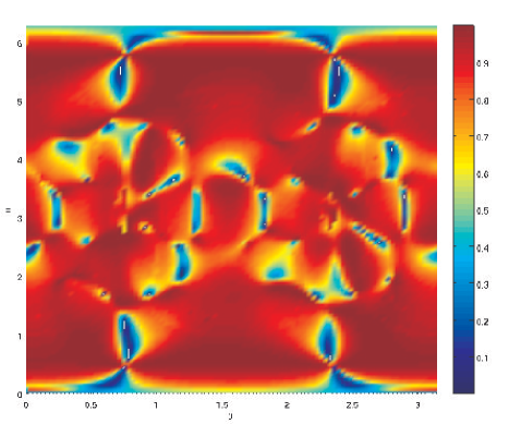
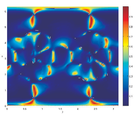
Figure 5: Population of $\ket{0}$ and $\ket{1}$ vibrational states after the high harmonic process as a function of angle for the $T_{2g}$ normal mode transforming like $xy$.

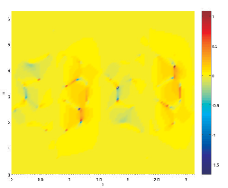
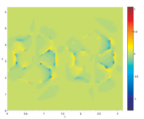
Figure 6: Modulation of HHG signal resulting in final vibrational state $\ket{0}$ as a function of angle for the $T_{2g}$ normal mode transforming like $xy$. a) real component of modulation b) imaginary component of modulation

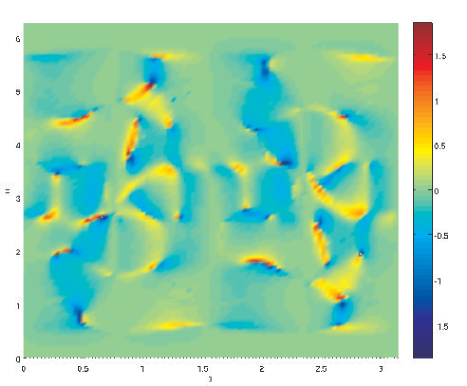
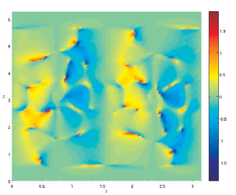
Figure 7: Modulation of HHG signal resulting in final vibrational state $\ket{1}$ as a function of angle for the $T_{2g}$ normal mode transforming like $xy$. a) real component of modulation b) imaginary component of modulation

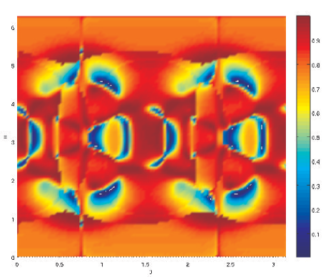
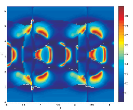
Figure 8: Population of $\ket{0}$ and $\ket{1}$ vibrational states after the high harmonic process as a function of angle for the $E_{g}$ normal mode transforming like $2z^{2}-x^{2}-y^{2}$.

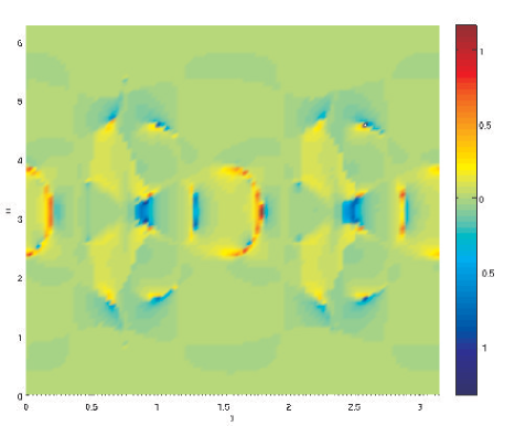
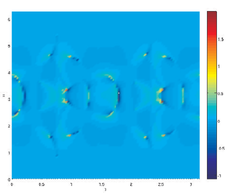
Figure 9: Modulation of HHG signal resulting in final vibrational state $\ket{0}$ as a function of angle for the $E_{g}$ normal mode transforming like $2z^{2}-x^{2}-y^{2}$. a) real component of modulation b) imaginary component of modulation

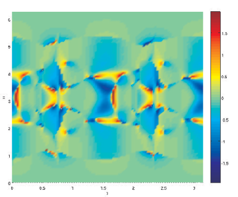
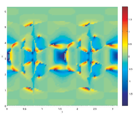
Figure 10: Modulation of HHG signal resulting in final vibrational state $\ket{1}$ as a function of angle for the $E_{g}$ normal mode transforming like $2z^{2}-x^{2}-y^{2}$. a) real component of modulation b) imaginary component of modulation.

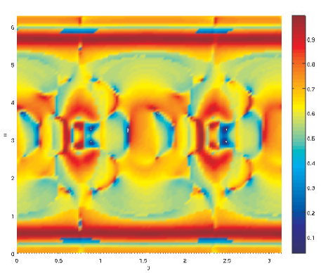
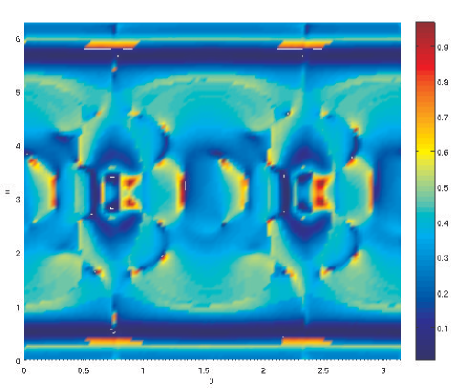
Figure 11: Population of $\ket{0}$ and $\ket{1}$ vibrational states after the high harmonic process as a function of angle for the totally symmetric $A_{1g}$ mode.

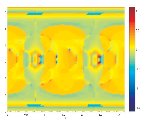
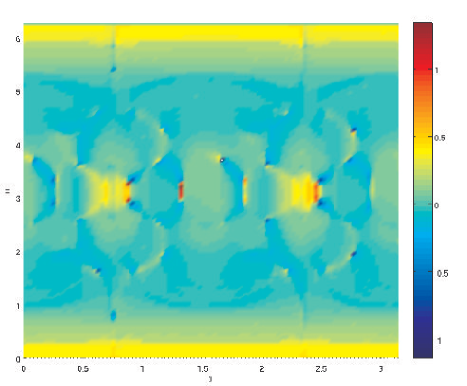
Figure 12: Modulation of HHG signal resulting in final vibrational state $\ket{0}$ as a function of angle for the totally symmetric $A_{1g}$ mode. a) real component of modulation b) imaginary component of modulation

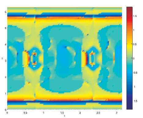
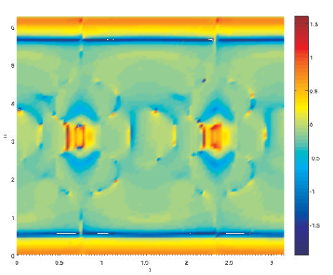
Figure 13: Modulation of HHG signal resulting in final vibrational state $\ket{1}$ as a function of angle for the totally symmetric $A_{1g}$ mode. a) real component of modulation b) imaginary component of modulation.

A previous workWalters et al. (2007) compared only the angular averaged modulation of the entire signal to experiment, by calculating the modulation to first order in raising and lowering operators. For the present work, the modulation at a particular molecular orientation was calculated using the full transfer matrices $\underline{I}$, $\underline{R}$ and $\underline{M}$. The resulting vibrational state populations and modulations of the different components of the HHG signal show a rich angular structure which is lost upon angular averaging.

Note that all calculations presented here have used the separable approximation of Eq.3 for the amplitudes of the different vibrational modes. This is expected to be accurate to the extent that the ground vibrational state dominates, meaning that for the amplitudes that we have calculated here, the higher-order nonseparable pathways are at least beginning to become important, which diminishes the validity of this approximation. Nevertheless, it is still expected to have at least qualitative and perhaps even semi-quantitative validity for the range of parameters studied here.

Using the separable approximation, the final populations of the $\ket{0}$ and $\ket{1}$ for each normal mode and their modulation as a function of time were calculated as a function of angle using equation 17. Figures 5,6,7 show final state populations and the real and imaginary components of the modulation as a function of angle for the $T_{2g}$ mode transforming like $xy$. Figures 8,9,10 show final state populations and modulations for the $E_{g}$ mode transforming like $2z^{2}-x^{2}-y^{2}$, while Figures 11,12,13 show final populations and modulation fractions for the totally symmetric $A_{1g}$ mode. In all three modes, the population of the $\ket{1}$ vibrational state is modulated much more heavily than the population of the $\ket{0}$ state.

A noteworthy feature of these figures is that in regions where Raman excitation during the HHG pulse is weak, the modulation of the HHG signal due to $d_{0}^{*}d_{0}$ (ie, HHG processes ending with the molecule in the ground vibrational state) tends to cancel modulation due to $d_{1}^{*}d_{1}$ (leaving the molecule in the first vibrational state). For this reason, angle-averaged modulations of the overall HHG signal due to the T_2g and E_g normal modes give almost zero overall modulation, while the modulations of the $d_{0}^{*}d_{0}$ or $d_{1}^{*}d_{1}$ give a large fractional modulation. (The A_1g mode experiences strong Raman excitation at all molecular orientations, and experiences less cancellation as a result.)

It is not clear why this cancellation is not observed in the experiment, where the T_2g mode is typically the most visible wag . This could arise due to a variety of causes, such as preferential detection of the $d_{1}^{*}d_{1}$ component of the signal relative to the $d_{0}^{*}d_{0}$ component, or some mechanism changing the phase between the modulation of the two components and thereby eliminate the cancellation. Table 3 shows the fraction of molecules finishing the HHG process in the $\ket{0}$ and $\ket{1}$ states, while table 1 compares the modulation of the $d_{0}^{*}d_{0}$ and $d_{1}^{*}d_{1}$ components of the signal, the modulation of the total signal, and the two experimental runs which were able to detect modulations at all three vibrational frequencies. Tables 4 and 2 shows the same information when the HHG process is allowed to populate vibrational states up to $\ket{4}.$ It is apparent from Table 4 that including higher vibrational states of the T_2g and E_g modes do not greatly affect the calculated modulations. For the $A_{1g}$ mode, which undergoes stronger Raman excitation, the presence of $\ket{2}$ and higher vibrational states does become important.

Table 1: Peak-to-peak Modulation, Theory vs. Experiment (2 state model)

Mode	Experiment 1	Experiment 2	$\ket{0}$	$\ket{1}$	Total Signal
A1g	.06	.105	.0439	.187	.0246
T2g	.105	.122	.0010	.236	.0016
Eg	.025	.029	.0255	.121	.0020

Table 2: Peak-to-peak Modulation, Theory vs. Experiment (5 state model)

Mode	$\ket{0}$	$\ket{1}$	$\ket{2}$	$\ket{3}$	$\ket{4}$	Total modulation
A1g	.0495	.249	.508	1.01	1.44	.0901
T2g	.0099	.232	.708	1.45	1.84	.0011
Eg	.0264	.142	.907	1.55	1.88	.0071

Table 3: Vibrational State Population After HHG process (2 state model)

Mode	$\ket{0}$ pop.	$\ket{1}$ pop.
A1g	0.71	0.29
T2g	0.87	0.13
Eg	0.69	0.33

Table 4: Vibrational State Population After HHG process (5 state model)

Mode	$\ket{0}$ pop.	$\ket{1}$ pop.	$\ket{2}$ pop.	$\ket{3}$ pop.	$\ket{4}$ pop.
A1g	.611	.310	.0719	7.03$\times 10^{-3}$	4.37$\times 10^{-4}$
T2g	.955	.0438	6.92$\times 10^{-4}$	7.90$\times 10^{-6}$	8.73$\times 10^{-8}$
Eg	.826	.168	5.91$\times 10^{-3}$	1.63$\times 10^{-4}$	3.59$\times 10^{-6}$

Although the agreement with experiment is not perfect, it is nevertheless significant that the simple model of vibrational interference presented here agrees with experiment to the correct order of magnitude. This is particularly notable in light of conventional Raman spectroscopy, in which the A_1g peak is 20 times more prominent than the others. It is difficult to precisely gauge the agreement of theory and experiment, due to the paucity of experimental data. Peak-to-peak modulations vary extensively from one experimental run to another wag with this SF₆ experiment. The modulation at 525 $cm^{-1}$, corresponding to the T_2g mode, appears most prominently in the experimental data, yet it gives the smallest modulation in this treatment. The prominence of the T_2g mode modulation may suggest that the off-diagonal Jahn-Teller coupling $V_{T_{2g}}$ is larger than obtained in the present calculations. Alternatively, it may be necessary to model the experiment in more detail – i.e. to incorporate the spatially-varying laser intensity, the uncontrolled carrier envelope phase, the combination of multiple laser half cycles, etc – beyond that which has been included in the present theoretical description.

VI Conclusions

The problem of high harmonic generation in molecules can be conceptually separated into two parts: the evolution of the continuum electron, and the evolution of the internal (vibrational) wavefunction of the parent ion. This paper describes the evolution of the continuum electron in a model which combines a semiclassical treatment of the propagation with a fully quantum mechanical description of the electron-molecule scattering. This flexible and robust model has a simple conceptual link to existing semiclassical models, yet it allows for a sophisticated treatment of the complicated electron-molecule scattering. The internal dynamics of the parent ion are tracked throughout the high harmonic process. Together, these two innovations serve to give an unprecedented view of high harmonic generation in a comparatively large, complicated molecule with many internal degrees of freedom, giving results which agree with experiment to within an order of magnitude.

The possibility that high harmonic generation may serve as an ultrafast interferometric probe of a molecular vibrational wavefunction is extremely promising. Such a wavefunction need not be prepared by an initial Raman pulse, as was the case for the JILA experiment. Instead, a preparatory pulse could photoionize a molecule, excite it to a higher electronic state, or trigger the beginning of some other chemical process. In this way, vibrational wavepacket evolution during chemical processes could be observed as it happens.

VII Acknowledgments

We thank the group of H. Kapteyn and M. Murnane for helpful discussions. This work was supported in part by the Office of Science, Department of Energy, and in part by the NSF EUV Engineering Research Center.

VIII Appendix: Tunneling Ionization

In this approximate treatment, the wavefunction in the forbidden region is found using the WKB connection formulas. As is illustrated in Figure 4, the classically forbidden region is defined by two turning points, $a$ and $b$, aligned in the downfield direction, between which $V(x)-E>0$. The slope of $V(x)$ is $C_{1}>0$ at the inner turning point $a$ and $C_{2}<0$ at the outer turning point $b$.

Near turning point $a$, $k^{2}(x)\equiv 2m(E-V(x))\approx C_{1}(a-x)$ and the time independent Schrödinger equation is

$$\psi^{\prime\prime}+k^{2}(x)\psi=0,$$ (36)

which has solutions near $x=a$ of

$$\psi(x)=\text{Ai}(\frac{C_{1}(x-a)}{C_{1}^{2/3}})b_{1}+\text{Bi}(\frac{C_{1}(x-a)}{C_{1}^{2/3}})b_{2}$$ (37)

where Ai and Bi are Airy functions, asymptotically behaving like

$$\text{Ai}(z)\Rightarrow_{z\rightarrow\infty} (2\pi)^{-1/2}z^{-1/4}\exp[\frac{-2}{3}z^{3/2}]$$ (38)

$$\text{Ai}(z)\Rightarrow_{z\rightarrow-\infty} \pi^{-1/2}(-z)^{-1/4}\sin(\frac{2}{3}(-z)^{3/2}+\pi/4)$$ (39)

$$\text{Bi}(z)\Rightarrow_{z\rightarrow\infty} \pi^{-1/2}z^{-1/4}\exp(\frac{2}{3}z^{3/2})$$ (40)

$$\text{Bi}(z)\Rightarrow_{z\rightarrow-\infty} \pi^{-1/2}(-z)^{-1/4}\cos(\frac{2}{3}(-z)^{3/2}+\pi/4)$$ (41)

where $z=C_{1}^{1/3}(x-a)$

Similarly, near $x=b$

$$\psi(x)=\text{Ai}(C_{2}^{1/3}(b-x))d_{1}+\text{Bi}(C_{2}^{1/3}(b-x))d_{2}$$ (42)

Under the barrier but away from the turning points, the WKB wavefunction is given by

$$\begin{split}\psi(x)=\pi^{-1/2}|k(x)|^{-1/2}\exp(\int_{a}^{x}|k(x^{\prime})|dx^{\prime})\sin(\phi)-\\ \frac{1}{2}|k(x)|^{-1/2}\exp(-\int_{a}^{x}|k(x^{\prime})|dx^{\prime})\cos(\phi)\end{split}$$ (43)

for some value of $\phi$.

Setting $\int_{a}^{b}|k(x^{\prime}|dx^{\prime}\equiv\Gamma$, note that

$$\int_{a}^{x}|k(x^{\prime})|dx^{\prime}=\Gamma-\int_{x}^{b}|k(x^{\prime}|dx^{\prime}$$ (44)

and for x close to $b$

$$\int_{b}^{x}k(x^{\prime})dx^{\prime}=\frac{2}{3}C_{2}^{1/2}(x-b)^{3/2}$$ (45)

Connecting the asymptotic forms of the Airy functions to the WKB solution in the forbidden region gives the solution for $x\approx b$ as

$$\begin{split}\psi(x)=_{x\approx b}2C_{2}^{-1/6}\sin(\phi)e^{\Gamma}\text{Ai}(C_{2}^{1/3}(b-x))-\\ \frac{1}{2}C_{2}^{-1/6}\cos(\phi)e^{-\Gamma}\text{Bi}(C_{2}^{1/3}(b-x)),\end{split}$$ (46)

giving a scattering phaseshift $\delta$ of

$$\delta=\tan^{-1}(4e^{2\tau}\tan(\phi))$$ (47)

yielding a resonance at $\phi\approx 0$, $\delta\approx\frac{pi}{2}$

Similar logic gives the wavefunction for $x\approx a$

$$\begin{split}\psi(x)=_{x\approx a}C_{1}^{-1/6}\sin(\phi)\text{Bi}(C_{1}^{1/3}(x-a))-\\ C_{1}^{1/6}\cos(\phi)\text{Ai}(C_{1}^{1/3}(x-a))\end{split}$$ (48)

Finally, setting $\phi=0$, the ratio of the tunneling wavefunction at the outer turning point to the tunneling wavefunction at the inner turning point is

$$\frac{\psi(x=b)}{\psi(x=a)}=\frac{1}{2}e^{-\Gamma}(|\frac{C_{1}}{C_{2}}|)^{1/6}\frac{\text{Bi}(0)}{\text{Ai}(0)}$$ (49)

References

- Wagner et al. (2006) N. Wagner, A. Wüest, I. Christov, T. Popmintchev, X. Zhou, M. Murnane, and H. Kapteyn, Proc. Natl. Acad. Sci. U.S.A. 103, 13279 (2006).
- Walters et al. (2007) Z. Walters, S. Tonzani, and C. Greene, J. Phys. B 40, F277 (2007).
- Frisch et al. (1998) M. Frisch, G. Trucks, H. Schlegel, G. Scuseria, M. Robb, J. Cheeseman, V. Zakrzewski, J. Montgomery Jr, R. Stratmann, J. Burant, et al., Inc., Pittsburgh, PA (1998).
- Dunning Jr (1989) T. Dunning Jr, J. Chem. Phys. 90, 1007 (1989).
- Estreicher and Estle (1985) S. Estreicher and T. L. Estle, Phys. Rev. B 31, 5616 (1985).
- Moffitt and Thorson (1957) W. Moffitt and W. Thorson, Phys. Rev. 108, 1251 (1957).
- Bersuker and Borisovich (1984) I. Bersuker and I. Borisovich, The Jahn-Teller effect and vibronic interactions in modern chemistry (Plenum Press, 1984).
- Corkum (1993) P. Corkum, Phys. Rev. Lett. 71, 1994 (1993).
- Lewenstein et al. (1994a) M. Lewenstein, P. Balcou, M. Y. Ivanov, A.L’Huillier, and P. B. Corkum, Phys. Rev. A 49, 2117 (1994a).
- Lewenstein et al. (1994b) M. Lewenstein, P. Balcou, M. Ivanov, A. L’Huillier, and P. Corkum, Phys. Rev. A 49, 2117 (1994b).
- Kazamias and Balcou (2004) S. Kazamias and P. Balcou, Physical Review A 69, 063416 (2004).
- Walters et al. (2008) Z. B. Walters, S. Tonzani, and C. H. Greene, J. Phys. Chem. A 112, 9439 (2008).
- Le et al. (2008) A. Le, R. D. Picca, P. D. Fainstein, D. A. Telnov, M. Lein, and C. D. Lin, J. Phys. B 41, 081002 (2008).
- Smirnova et al. (2008) O. Smirnova, M. Spanner, and M. Ivanov, Phys. Rev. A 77, 033407 (2008).
- Miller (2001) W. H. Miller, J. Phys. Chem. A 105, 2942 (2001).
- Nakamura (2005) H. Nakamura, J. Theor. Comp. Chem. 4, 127 (2005).
- Gutzwiller (1990) M. Gutzwiller, Chaos in Classical and Quantum Mechanics (Springer, New York, 1990).
- Tonzani and Greene (2005) S. Tonzani and C. H. Greene, J. Chem. Phys. 122, 014111 (2005).
- Tonzani and Greene (2006) S. Tonzani and C. H. Greene, J. Chem. Phys. 124, 054312 (2006).
- Tonzani (2007) S. Tonzani, Comp. Phys. Comm. 176, 146 (2007).
- Goldstein et al. (2002) H. Goldstein, C. Poole, J. Safko, and S. Addison, Classical Mechanics, Third Edition (Addison Wesley, 2002).
- (22) N. Wagner, private communication.