The Sigma Model on
Complex Projective Superspaces

The sigma model on projective superspaces $\text{$\mathbb{CP}$}^{S-1|S}$ gives rise to a continuous family of interacting 2D conformal field theories which are parametrized by the curvature radius $R$ and the theta angle $\theta$. Our main goal is to determine the spectrum of the model, non-perturbatively as a function of both parameters. We succeed to do so for all open boundary conditions preserving the full global symmetry of the model. In string theory parlor, these correspond to volume filling branes that are equipped with a monopole line bundle and connection. The paper consists of two parts. In the first part, we approach the problem within the continuum formulation. Combining combinatorial arguments with perturbative studies and some simple free field calculations, we determine a closed formula for the partition function of the theory. This is then tested numerically in the second part. There we extend the proposal of [arXiv:0908.1081] for a spin chain regularization of the $\text{$\mathbb{CP}$}^{S-1|S}$ model with open boundary conditions and use it to determine the spectrum at the conformal fixed point. The numerical results are in remarkable agreement with the continuum analysis.

DESY 09-120 0908.0878

1 Introduction

Sigma models with target space supersymmetry are of much recent interest. They possess a number of truly remarkable properties. Most importantly, many of them come in continuous families with vanishing $\beta$-function, i.e. they provide examples of (non-unitary) 2-dimensional conformal field theories with continuously varying exponents. There are several series of such models that arise from compact symmetric superspaces, including the sigma model on the odd-dimensional superspheres $S^{2S+1|2S}$ and on the complex projective superspaces $\text{$\mathbb{CP}$}^{S-1|S}$. Their systematic investigation was initiated in [1]. More recently, the superspheres have been reconsidered both through numerical and algebraic investigations of lattice discretizations [2, 3] and within the continuum formulation [4]. In particular, it was shown that the conformal weights of fields with open boundary conditions possess a very simple dependence on the curvature radius of the supersphere. In fact, when Neumann boundary conditions are imposed on both ends of the strip, the boundary partition function can be computed exactly. The resulting formula provides strong evidence for a remarkable new non-perturbative (in the radius $R$ or, equivalently, the sigma model coupling $g_{\sigma}$) duality between the sigma model on superspheres and the OSP($2S+2|2S$) Gross-Neveu model. It generalizes the famous duality between the compactified free boson and the massless Thirring model.

The aim of this note is to extend the investigations of [2, 4] to sigma models with target space $\text{$\mathbb{CP}$}^{S-1|S}$. The sigma model on complex projective superspaces gives rise to a 2-parameter family of conformal fields theories with central charge $c=-2$. In addition to the sigma model coupling $g_{\sigma}$ (or radius $R$) one can also introduce a theta term with arbitrary coefficient $\theta$. There are several reasons to be interested in these models. To begin with, the spaces $\text{$\mathbb{CP}$}^{S-1|S}$ are the simplest examples of Calabi-Yau supermanifolds. Supersymmetric sigma models on these spaces have been investigated by several authors (see e.g. [5, 6, 7, 8, 9, 10]) after Witten had proposed the open topological B-model on $\text{$\mathbb{CP}$}^{3|4}$ as a candidate for a string theoretic description of N=4 super Yang-Mills theory [11]. Further motivation comes from one of the ramifications of the $AdS/CFT$ correspondence. According to a recent conjecture in [12], the IR fixed point of the effective gauge field theory on a stack of D2 branes is dual to string theory on $AdS_{4}\times\text{$\mathbb{CP}$}^{3|4}$. Though our findings for the sigma model on $\text{$\mathbb{CP}$}^{S-1|S}$ do not possess direct applications to the spectrum of string theory, our study throws light on some basic features such as e.g. the issue of instanton corrections to physical quantities. Since the bosonic base of $\text{$\mathbb{CP}$}^{S-1|S}$ has a non-trivial second cohomology $H_{2}$, world-sheet instanton solutions to the classical sigma model do exist and signal the possibility of non-perturbative effects. These seem well worth a more detailed investigation, both in the $\text{$\mathbb{CP}$}^{S-1|S}$ sigma models and the string background $AdS_{4}\times\text{$\mathbb{CP}$}^{3|4}$. A third motivation we want to mention is related to the theory of quantum Hall plateau transitions. The model we are about to study may be considered as a compact relative of the sigma model $\text{U}(1,1|2)/\text{U}(1|1)\times\text{U}(1|1)$ at $\theta=\pi$ that has been extensively studied in this context in [13, 14]. Some of our constructions and results suggest interesting extensions to the non-compact model. We shall come back to the last two applications in the concluding section.

Let us now describe the content of the paper and its main results. Our work is split into two parts, one on the continuum formulation, the other on numerical studies of a lattice discretization. Our presentation begins with a review of the classical sigma model on $\text{$\mathbb{CP}$}^{S-1|S}$. Since we are mostly interested in world-sheets with boundaries, particular attention will be paid to boundary conditions. In particular, we analyze the possible $\text{U}(S\,|S)$ symmetric boundary conditions. As we shall discuss, these are associated with complex line bundles on $\text{$\mathbb{CP}$}^{S-1|S}$ and hence they are labelled by an integer $M$. In Section 3 we analyze the quantum theory in the limit of infinite radius $R$ (vanishing sigma model coupling $g_{\sigma}$). We start our presentation by reviewing the state space of a particle on $\text{$\mathbb{CP}$}^{1|2}$ in the presence of a monopole gauge field. One of the two different descriptions we provide generalizes straightforwardly to the full quantum field theory. The main goal of section 3 is to construct and analyze the partition function (3.18) of the boundary field theory at $R=\infty$. Our strategy then is to deform the partition function from $R=\infty$ to finite $R$. To this end we adapt the background field expansion to the sigma model on $\text{$\mathbb{CP}$}^{S-1|S}$and explain how to compute boundary 2-point functions. As in the case of superspheres, there are remarkable cancellations in the expansion for boundary conformal weights. These suggest an exact expression (4.2) for the partition function of the model at finite radius and for arbitrary value of the $\theta$ angle. After explaining the various ingredients of this formula, we extract a list of consequences that will be confronted with numerical tests.

In the second part, we consider a lattice version of the sigma model on $\text{$\mathbb{CP}$}^{S-1|S}$. This lattice version was first studied in [15]. Our approach does not rely on direct discretization of the action and Monte Carlo simulations, but rather on the general relation between sigma models and spin chains. We are thus led to study an ”antiferromagnetic” spin chain where the degrees of freedom take values in an alternating sequence of $\text{u}(S\,|S)$  modules $V$ and $V^{\star}$. By allowing interactions between nearest neighbors as well as second nearest neighbors, we are able to recover the spectrum of the $\text{$\mathbb{CP}$}^{S-1|S}$ model, and to check most predictions from the continuum theory. In particular, we find good agreement with our proposal for the exact partition function (4.2), and we determine the running coupling constant $g_{\sigma}^{2}$ in terms of the lattice parameters. We also come up with a natural lattice version of the boundary conditions of the sigma model associated with non trivial complex line bundles.

Part I: Continuum Theory
In the first part we shall approach the $\text{$\mathbb{CP}$}^{S-1|S}$ model through its continuum formulation. Target space supersymmetry will allow us to find exact expressions for the conformal weights of boundary fields as a function of radius $R$ and theta angle $\theta$.

2 The Sigma Model on Projective Superspace

The aim of this section is to review some facts about the complex projective superspace $\text{$\mathbb{CP}$}^{S-1|S}$ and the non-linear sigma model thereon. In the first subsection we discuss two different formulations of the theory. The first one involves a constraint and it is manifestly $\text{U}(S\,|S)$ invariant. There exists an alternative description, in which the constraint is solved at the expense of breaking the $\text{U}(S\,|S)$ symmetry down to U($S-1|S$). Both formulations will play some role in the subsequent analysis. The second subsection contains a comprehensive analysis of $\text{U}(S\,|S)$ symmetric boundary conditions. We shall argue that there exists an infinite family of such boundary conditions, one for each integer $M$. They correspond to the choice of a complex line bundle in $\text{$\mathbb{CP}$}^{S-1|S}$ along with a connection one-form $A_{M}$. For $S=2$ the connection one-form is a supersymmetric version of the gauge field produced by a Dirac monopole of charge $M$.

2.1 The sigma model on $\text{$\mathbb{CP}$}^{S-1|S}$

Complex projective superspaces $\text{$\mathbb{CP}$}^{S-1|S}$ are built in a way that resembles closely the construction of their bosonic cousins. We begin with flat superspace $\mathbb{C}^{S|S}$. The $S$ complex bosonic coordinates are denoted by $z_{a}$ and we use $\xi_{a}$ for the $S$ fermionic directions. Within the flat complex superspace we consider the odd (real) dimensional supersphere defined by the equation

$$\sum_{a=1}^{S}z_{a}z_{a}^{\ast}+\sum_{a=1}^{S}\xi_{a}\xi_{a}^{\ast}=1\ \ .$$ (2.1)

The supersphere $S^{2S-1|2S}$ carries an action of U(1) by simultaneous phase rotations of all bosonic and fermionic coordinates,

$$z_{a}\ \longrightarrow\ e^{i\varpi}z_{a}\ \ \ \ \ ,\ \ \ \ \xi_{a}\ \longrightarrow\ e^{i\varpi}\xi_{a}\ \ .$$ (2.2)

Note that this transformation indeed leaves the constraint invariant. The complex projective superspace $\text{$\mathbb{CP}$}^{S-1|S}$ is the quotient space $S^{2S-1|2S}$​/U(1).

Functions on the supersphere $S^{2S-1|2S}$ carry an action of the the Lie supergroup $\text{U}(S\,|S)$. These transformations include the phase rotations (2.2) which act trivially on $\text{$\mathbb{CP}$}^{S-1|S}$. Hence, the stabilizer subalgebra of a point on the projective superspace is given by u(1) $\times$ u($S-1|S$) where the first factor corresponds to the action (2.2). We conclude that

$$\text{$\mathbb{CP}$}^{S-1|S}\ =\ \text{$\text{U}(S\,|S)$}/\left(\,\text{U(1) $\times$ U($S-1|S$)}\right)\ \ .$$ (2.3)

Their simplest representative is $\text{$\mathbb{CP}$}^{0|1}$  i.e. the space with just two real fermionic coordinates. The sigma model with this target space is equivalent to the theory of two symplectic fermions, which has been extensively investigated, as for example in [16, 17]. Let us also recall that for $S=2$, the bosonic base of $\text{$\mathbb{CP}$}^{1|2}$ is a 2-sphere. The superspace $\text{$\mathbb{CP}$}^{1|2}$$=S^{2}\times\mathbb{C}^{2}$ is a bundle with fermionic complex 2-dimensional fibers. As for their bosonic cousins, the second homology group $H_{2}(\text{$\mathbb{CP}$}^{S-1|S})=\mathbb{Z}$ of complex projective superspaces is non-trivial. Consequently, $\text{$\mathbb{CP}$}^{S-1|S}$ supports line bundles whose second Chern-class is characterized by an integer $M\in\mathbb{Z}$. In the case of $\text{$\mathbb{CP}$}^{1|2}$, the expression for the corresponding connection one-form is well known from the theory of Dirac monopoles. We shall often refer to the integer $M$ as the monopole number.

The construction of the sigma model on $\text{$\mathbb{CP}$}^{S-1|S}$ can be inferred from the geometric construction we outlined above. The model involves a field multiplet $Z_{\alpha}=Z_{\alpha}(z,\bar{z})$ with $S$ bosonic components $Z_{\alpha}=z_{\alpha},\alpha=1,\dots,S,$ and the same number of fermionic fields $Z_{\alpha}=\xi_{\alpha-S},\alpha=S+1,\dots,2S$. To distinguish between bosons and fermions we introduce from now on a grading function $|\cdot|$, which is 0 when evaluated on the labels of bosonic and 1 on the labels of fermionic quantities. In addition we also need a non-dynamical U(1) gauge field $a$. With this field content, the action takes the form

$$S\ =\ \frac{1}{2g_{\sigma}^{2}}\int d^{2}z(\partial_{\mu}-ia_{\mu})Z_{\alpha}^{\dagger}(\partial_{\mu}+ia_{\mu})Z_{\alpha}-\frac{i\theta}{2\pi}\int d^{2}z\epsilon^{\mu\nu}\partial_{\mu}a_{\nu}$$ (2.4)

and the fields $Z_{\alpha}$ are subject to the constraint $Z_{\alpha}^{\dagger}Z_{\alpha}=1$. The integration over the abelian gauge field can be performed explicitly and it leads to the replacement

$$a_{\mu}\ =\ \frac{i}{2}\left[Z_{\alpha}^{\dagger}\partial_{\mu}Z_{\alpha}-(\partial_{\mu}Z_{\alpha}^{\dagger})Z_{\alpha}\right]\ \ .$$ (2.5)

The term multiplied by $\theta$ does not contribute to the equations of motion for $a_{\mu}$. As its bosonic counterpart, the $\text{$\mathbb{CP}$}^{S-1|S}$ sigma model on a closed surface possesses instanton solutions. The corresponding instanton number is computed by the term that multiplies the parameter $\theta$. Since it is integer valued, the parameter $\theta=\theta+2\pi$ can be considered periodic as long as the world-sheet has no boundary.

In order to pass to our second formulation of the $\text{$\mathbb{CP}$}^{S-1|S}$ model we employ the gauge freedom to solve the constraint $Z_{\alpha}^{\dagger}Z_{\alpha}=1$ as follows

$$Z_{1}=Z^{\dagger}_{1}\ =\ \frac{1}{\sqrt{1+w^{\dagger}\cdot w}},\quad Z_{i+1}\ =\ \frac{w^{i}}{\sqrt{1+w^{\dagger}\cdot w}},\quad Z^{\dagger}_{i+1}\ =\ \frac{w^{\bar{\imath}}}{\sqrt{1+w^{\dagger}\cdot w}}\ .$$ (2.6)

Thereby we have parametrized the target space $\text{$\mathbb{CP}$}^{S-1|S}$ through a set of $S-1$ complex bosonic components $w_{1},\dots,w_{S-1}$ and a set of $S$ complex fermionic ones $w_{S},\dots,w_{2S-1}$. Plugging this parametrization (2.6) back into the action (2.4) we obtain an unconstrained reformulation of the $\text{$\mathbb{CP}$}^{S-1|S}$ sigma model

$$S\ =\ \frac{1}{2g_{\sigma}^{2}}\int d^{2}z\,g_{i\bar{\jmath}}\partial_{\mu}w^{\bar{\jmath}}\partial_{\mu}w^{i}+\frac{i\theta}{2\pi}\int d^{2}z\,\epsilon^{\mu\nu}ig_{i\bar{\jmath}}\partial_{\nu}w^{\bar{\jmath}}\partial_{\mu}w^{i},$$ (2.7)

where $g_{i\bar{\jmath}}$ is the canonical Fubini-Study metric on $\text{$\mathbb{CP}$}^{S-1|S}$

$$g_{i\bar{\jmath}}\ =\ \frac{\delta_{ij}}{1+w^{\dagger}\cdot w}-\frac{(-1)^{|j|}w^{\bar{\imath}}w^{j}}{(1+w^{\dagger}\cdot w)^{2}}\ .$$ (2.8)

The disadvantage of this reformulation is the non-linear action of the $\text{U}(S\,|S)$ supergroup on the projective coordinates $w,\bar{w}$. Let us recall in passing that the Fubini-Study metric on $\text{$\mathbb{CP}$}^{S-1|S}$ determines the following Kähler two-form

$$\omega\ =\ d^{2}z\,\epsilon^{\mu\nu}ig_{i\bar{\jmath}}\partial_{\nu}w^{\bar{\jmath}}\partial_{\mu}w^{i}\ =\ -ig_{i\bar{\jmath}}dw^{\bar{\jmath}}\wedge dw^{i}\ .$$ (2.9)

The Kähler form is properly normalized and generates the second integral cohomology group of $\text{$\mathbb{CP}$}^{S-1|S}$, that is

$$\int\frac{\omega}{2\pi}\ =\ 1\ .$$ (2.10)

It follows, as stated before, that our bulk model is not affected if we shift $\theta$ by integer multiples of $2\pi$, i.e. we can restrict the parameter $\theta$ to the interval $\theta\in[-\pi,\pi[$.

2.2 Action of the boundary model

We are now going to discuss $\text{U}(S\,|S)$ symmetric boundary conditions of the $\text{$\mathbb{CP}$}^{S-1|S}$ model. For readers used to the string theoretic concept of branes and the geometric classification of boundary conditions, the final outcome is not surprising. Note that $\text{$\mathbb{CP}$}^{S-1|S}$ admits a natural left action of $\text{U}(S\,|S)$. Since $\text{$\mathbb{CP}$}^{S-1|S}$ is homogeneous under this action, any $\text{U}(S\,|S)$ symmetric brane must be volume filling. But branes are not simply (sub-)manifolds in target space. They also carry a bundle ${\cal L}$ with connection $A$. In the case at hand, there is an infinite family of complex line bundles ${\cal L}_{M}$ on $\text{$\mathbb{CP}$}^{S-1|S}$ which are parametrized by the integer $M\in\mathbb{Z}$. To ensure $\text{U}(S\,|S)$ invariance, the connection $A_{M}$ must have constant curvature $\Omega_{M}$. Consequently, its curvature is proportional to the Kähler form $\omega$, i.e. $\Omega_{M}\sim M\omega$. We shall now see how these geometric insights manifest themselves in the world-sheet description. Our presentation will not make any more reference to string theoretic notions.

We want to consider the $\text{$\mathbb{CP}$}^{S-1|S}$ sigma model on a world-sheet $\Sigma$ with boundary. The choice we have in mind is a strip $\Sigma=[0,\pi]\times\mathbb{R}$ or, equivalently, the upper half of the complex plane $z=x+iy,y>0$. We are looking for boundary conditions which arise from adding boundary terms of the form

$$S_{b}\ =\ \int_{-\infty}^{0}dx\,\left(A^{L}_{i}(w,\bar{w})\partial_{x}w^{i}+A^{L}_{\bar{\imath}}(w,\bar{w})\partial_{x}w^{\bar{\imath}}\right)+\int_{0}^{\infty}dx\,\left(\,L\ \leftrightarrow\ R\,\right)$$ (2.11)

to the action (2.4, 2.7). Here, $A^{L(R)}=A^{L(R)}_{i}dw^{i}+A^{L(R)}_{\bar{\imath}}dw^{\bar{\imath}}$ are one-forms which are at least locally defined on $\text{$\mathbb{CP}$}^{S-1|S}$. When we map the half plane back to the strip, points with $z=x>0$ are mapped to the right boundary while those with $z=x<0$ end up on the left side. To find consistent boundary conditions we require invariance of the total action $S_{t}=S+S_{b}$ with respect to arbitrary variations $\delta w^{i}(z,\bar{z})$. It follows that

$$g_{i\bar{\jmath}}\left(\frac{1}{2g_{\sigma}^{2}}\partial_{y}+\frac{\theta}{2\pi}\partial_{x}\right)w^{\bar{\jmath}} =\ 2\Omega^{L(R)}_{ij}\partial_{x}w^{j}+2\Omega^{L(R)}_{i\bar{\jmath}}\partial_{x}w^{\bar{\jmath}}$$ (2.12)

$$g_{\bar{\imath}j}\left(\frac{1}{2g_{\sigma}^{2}}\partial_{y}-\frac{\theta}{2\pi}\partial_{x}\right)w^{j} =\ 2\Omega^{L(R)}_{\bar{\imath}\bar{\jmath}}\partial_{x}w^{\bar{\jmath}}+2\Omega^{L(R)}_{\bar{\imath}j}\partial_{x}w^{j},$$

where $z=\bar{z}<0\,(>0)$ and $\Omega^{L(R)}$ is the curvature 2-form of the connection $A^{L(R)}$. It is globally defined on $\text{$\mathbb{CP}$}^{S-1|S}$ through

$$\Omega^{L(R)}=dA^{L(R)}\ =\ -\Omega^{L(R)}_{ij}dw^{j}\wedge dw^{i}-2\Omega^{L(R)}_{i\bar{\jmath}}dw^{\bar{\jmath}}\wedge dw^{i}-\Omega^{L(R)}_{\bar{\imath}\bar{\jmath}}dw^{\bar{\jmath}}\wedge dw^{\bar{\imath}}.$$ (2.13)

Before imposing the conditions of $\text{U}(S\,|S)$ symmetry, we note that our boundary conditions (2.12) should preserve the complex structure of the $\text{$\mathbb{CP}$}^{S-1|S}$  supermanifold. Consequently, the complex conjugate of the first equation in (2.12) must yield the second equation without any additional constraint. While applying this constraint one must take into account the reality condition of a scalar field in Euclidean space-time

$$w^{i}(z,\bar{z})^{*}\ =\ w^{\bar{\imath}}(1/z^{*},1/\bar{z}^{*}).$$ (2.14)

Thus, we conclude that the two equations in (2.12) are compatible if and only if $\Omega^{L(R)}$ is imaginary.

Boundary conditions (2.12) are said to preserve the global $\text{U}(S\,|S)$ symmetry if they are invariant with respect to an infinitesimal action of the supergroup. To give a precise meaning to this statement, let us note that the set of eqs. (2.12) can be interpreted as the vanishing condition of some real vector field $L$ on the left boundary, with components

$$L^{i} =\ \left(\frac{1}{2g_{\sigma}^{2}}\partial_{y}-\frac{\theta}{2\pi}\partial_{x}\right)w^{i}-2g^{i\bar{k}}\Omega^{L}_{\bar{k}\bar{\jmath}}\partial_{x}w^{\bar{\jmath}}-2g^{i\bar{k}}\Omega^{L}_{\bar{k}j}\partial_{x}w^{j},$$ (2.15)

$$L^{\bar{\imath}} =\ \left(\frac{1}{2g_{\sigma}^{2}}\partial_{y}+\frac{\theta}{2\pi}\partial_{x}\right)w^{\bar{\imath}}-2g^{\bar{\imath}k}\Omega^{L}_{kj}\partial_{x}w^{j}-2g^{\bar{\imath}k}\Omega^{L}_{k\bar{\jmath}}\partial_{x}w^{\bar{\jmath}}$$ (2.16)

and a similar expression for another real vector field $R$ on the right boundary. The global $\text{U}(S\,|S)$ invariance of the boundary conditions (2.12) is then equivalent to the invariance of the vector field $L,R$ with respect to the infinitesimal action of the $\text{u}(S\,|S)$ Lie superalgebra. In other words, the Lie derivative of the vector field (2.15) with respect to any $\text{u}(S\,|S)$ Killing vector must vanish. As world-sheet translations and global symmetry transformations commute, it follows that the 2-forms $\Omega^{L(R)}$ must be invariant. On the other hand, on any irreducible complex symmetric superspace, there is only one invariant closed 2-form, namely the Kähler form $\omega$. Hence, invariance of the boundary conditions with respect to the global symmetry requires that

$$\Omega^{L}\ =\ iM\omega\ \quad\ \quad,\quad\quad\Omega^{R}\ =\ iN\omega$$ (2.17)

where $\omega$ is the Kähler form (2.9). In the classical theory, the $M,N$ can assume any real value. For the associated path integral to be well defined, however, they must be integers. Even though this sections deals with the classical action, we shall assume $M,N\in\mathbb{Z}$ from now on. For later use it is convenient to re-write $L$ and $R$ in an index free notation,

$$L\ =\ \frac{1}{2g_{\sigma}^{2}}\partial_{y}+iJ\left(\frac{\theta}{2\pi}+M\right)\partial_{x}\quad,\quad R\ =\ \frac{1}{2g_{\sigma}^{2}}\partial_{y}+iJ\left(\frac{\theta}{2\pi}+N\right)\partial_{x}\ .$$ (2.18)

Here we have introduced the (globally well defined) complex structure $J$ on the tangent space of $\text{$\mathbb{CP}$}^{S-1|S}$. The components $L^{i}=dw^{i}(L)$ and $L^{\bar{\imath}}=dw^{\bar{\imath}}(L)$ are recovered from $L$ with the help of the canonical basis $dw^{i}$ and $dw^{\bar{\imath}}$ in the cotangent space. Note that $L$ and $R$ only contain a specific combination $\Theta_{1}=2M+\theta/\pi$ and, respectively, $\Theta_{2}=2N+\theta/\pi$. We conclude that the periodic variable $\theta$ of the bulk theory gets promoted to a real valued variable $\Theta$ in the boundary problem [18]. In the limit $g_{\sigma}\rightarrow 0$, the value of $\Theta$ is irrelevant. In other words, the boundary conditions are purely Neumann when we approach infinite radius.

Before we close this section, let us briefly write the boundary conditions in terms of the manifestly $\text{U}(S\,|S)$ covariant formulation (2.4) of our theory. In this case, the variations of the basic fields $Z_{\alpha}$ must be consistent with the constraint eq. (2.1),

$$(\delta Z^{\dagger}_{\alpha})Z_{\alpha}+Z_{\alpha}^{\dagger}\delta Z_{\alpha}=0\ \ .$$

In order for the boundary contributions to the variation of the action to vanish, we must impose the usual twisted Neumann boundary conditions of the type

$$\begin{split}(\partial_{y}+ia_{y})Z_{\alpha}&=\ \ \Theta_{1}g_{\sigma}^{2}(\partial_{x}+ia_{x})Z_{\alpha}\ ,\\[5.69054pt] (\partial_{y}-ia_{y})Z^{\dagger}_{\alpha}&=\ -\Theta_{1}g_{\sigma}^{2}(\partial_{x}-ia_{x})Z_{\alpha}^{\dagger}\end{split}$$ (2.19)

for $z=\bar{z}<0$ and a similar condition with $M$ replaced by $N$, i.e. $\Theta_{1}$ replaced by $\Theta_{2}$, along the right half $z=\bar{z}>0$ of the boundary. The parameters $\Theta_{1}=2M+\theta/\pi$ and $\Theta_{2}=2N+\theta/\pi$ are the same combination of the $\theta$ angle in the bulk and the monopole numbers $M,N$ that appeared in eq. (2.18).

So far we have only discussed the classical theory. Understanding the detailed properties of the associated quantum field theories is the main aim of the following sections. For the time being let us just mention that the non-linear sigma models on $\text{$\mathbb{CP}$}^{S-1|S}$ have been argued to possess vanishing $\beta$ function [1]. This means that they give rise to conformal quantum field theories for any choice of the two couplings $g_{\sigma}$ and $\theta$. The central charge of these models must agree with the central charge of the free field theory at $g_{\sigma}\sim 0$, i.e. all models of this type have $c=-2$.

3 Spectrum of the non-interacting sigma model

Our discussion of the quantum field theory will begin with the limiting case $g_{\sigma}=0$ in which all the interactions are turned off. To keep things explicit, we will restrict to the first non-trivial case with $S=2$. Most of what we are about to describe generalizes quite easily to higher dimensional projective superspaces. We want to investigate the spectrum of the $\text{$\mathbb{CP}$}^{1|2}$ model on the strip (or half-plane) with twisted Neumann boundary conditions imposed along the boundary. In more stringy terms this corresponds to considering volume filling branes which wrap the 2-sphere of $\text{$\mathbb{CP}$}^{1|2}$. In a first step we shall analyze the spectrum in the particle limit. Then, in the second step, we include derivative fields and construct a partition function for the theory in the limit of vanishing coupling $g_{\sigma}$.

3.1 Spectrum for a particle moving on $\text{$\mathbb{CP}$}^{1|2}$

The semiclassical or minisuperspace approximation amounts to considering the string as a point like object, that is to neglecting the $\sigma$ dependence of the fields $w^{i}(\tau,\sigma)$. Thereby, we reduce the field theory to a point particle problem. We shall discuss the quantization of this system in two different ways. In the first description we use the gauge fixed formulation of the theory in terms of variables $w^{i},w^{\bar{\imath}}$. The spectrum of the associated Hamiltonian is known from [19]. Our second approach employs the U(2$|$2) covariant formulation. Its results agree with the first treatment, but the U(2$|$2) covariant construction is extended more easily to the full field theory.

So, let us start from the action (2.7) and set all $\sigma$-derivatives to zero. Integrating out the transverse coordinate $\sigma$ of the strip $\Sigma=[0,\pi]\times\mathbb{R}$ we get the following particle theory

$$S\ =\ \int_{-\infty}^{\infty}d\tau\,\left(\frac{\pi}{2g_{\sigma}^{2}}g_{i\bar{\jmath}}\dot{w}^{\bar{\jmath}}\dot{w}^{i}+A_{i}\dot{w}^{i}+A_{\bar{\imath}}\dot{w}^{\bar{\imath}}\right)\ ,$$ (3.1)

where locally the connection one-form $A$ is the difference of the two one-forms $A^{R}$ and $A^{L}$, i.e.

$$A\ =\ A^{R}-A^{L}\ \ .$$ (3.2)

The classical Hamiltonian of this quantum mechanical system takes the following simple form

$$H\ =\ -\frac{2g_{\sigma}^{2}}{\pi}g^{i\bar{\jmath}}(\Pi_{i}-A_{i})(\Pi_{\bar{\jmath}}-A_{\bar{\jmath}})\ \ ,$$ (3.3)

where the canonical momenta are given by

$$\Pi_{i}\ =\ \frac{\pi}{2g_{\sigma}^{2}}g_{i\bar{\jmath}}\dot{w}^{\bar{\jmath}}+A_{i}\ ,\quad\Pi_{\bar{\imath}}\ =\ \frac{\pi}{2g_{\sigma}^{2}}g_{\bar{\imath}j}\dot{w}^{j}+A_{\bar{\imath}}\ \ .$$ (3.4)

We can now pass to the quantum theory through the usual canonical quantization, i.e. by replacing Poisson brackets with commutators,

$$[w^{i},\Pi_{j}]\ =\ [w^{\bar{\imath}},\Pi_{\bar{\jmath}}]\ =\ \delta^{i}_{j}\ \ .$$ (3.5)

Note that the factor $i$ of the usual commutation relations $[x^{i},p_{j}]=i\delta^{i}_{j}$ is missing because we are formulating the theory in Euclidean time $\tau=it$. For the quantization procedure to make sense, the one-form $A$ must be a connection on a complex line bundle over $\text{$\mathbb{CP}$}^{1|2}$, see [20]. This furnishes a quantization condition for the curvature of the connection,

$$dA\ =\ -il\omega$$ (3.6)

with $l$ any integer and $\omega$ the Kähler form on $\text{$\mathbb{CP}$}^{1|2}$. The space of sections of such bundles may be realized explicitly as equivariant functions $f(w,\bar{w})$ on $\text{$\mathbb{CP}$}^{1|2}$ with the property

$$f(e^{i\alpha}w,e^{-i\alpha}\bar{w})=e^{il\alpha}f(w,\bar{w})\ .$$ (3.7)

Taking into account (3.2) we get the condition that $l=M-N$ must necessarily be an integer. Hence, if we admit e.g. $A^{L}=0$ as a possible boundary conditions, mutual consistency requires $N\in\mathbb{Z}$. The quantized form of the classical Hamiltonian (3.3) is, up to a numerical prefactor, the Bochner-Laplacian $\Delta^{(l)}_{\text{$\mathbb{CP}$}^{S-1|S}}$ on the complex line bundle over $\text{$\mathbb{CP}$}^{1|2}$ with monopole charge $l\in\mathbb{Z}$

$$\hat{H}^{(l)}\ =\ -\frac{g_{\sigma}^{2}}{\pi}\Delta^{(l)}_{\text{$\mathbb{CP}$}^{S-1|S}}\ .$$ (3.8)

The eigenvalues of the Bochner-Laplacian on $\text{$\mathbb{CP}$}^{S-1|S}$ where studied in [19]. For the Hamiltonian we obtain

$$h_{l}(k)\ =\ \frac{g_{\sigma}^{2}}{\pi}\left(2k^{2}+(2k+|l|)(|l|-1)-l^{2}\right)\quad\mbox{ for }\ k\ =\ 0,1,2,\dots$$ (3.9)

From the spectrum we can read off which $\text{u}(2|2)$ multiplets are realized as sections of monopole bundles on $\text{$\mathbb{CP}$}^{1|2}$. We will list the corresponding representations of U(2$|$2) a bit later at the end of our second construction of the spectrum.

Let us now see how to reproduce the spectrum of the particle theory within the U(2$|$2) covariant formulation. As before, we depart from the space $\mathbb{C}^{2|2}$ with coordinates $Z=(z_{1},z_{2},\xi_{1},\xi_{2})$. The 4-tuple $Z$ transforms in the fundamental representation $V$ of $\text{u}(2|2)$. On the projective superspace $\text{$\mathbb{CP}$}^{1|2}$, the multiplet $Z$ and its conjugate $Z^{\dagger}$ obey the following constraint

$$Z^{\dagger}\cdot Z\ =\ 1\qquad.$$ (3.10)

Note that $Z^{\dagger}$ transforms in the dual fundamental representation $Z^{\dagger}\in V^{\star}$ so that the equation (3.10) is consistent with the $\text{u}(2|2)$ symmetry. Consequently, if we quotient the space of functions on $\mathbb{C}^{2|2}$ by the ideal that is generated from $Z^{\dagger}\cdot Z-1$, we end up with some non-trivial $\text{u}(2|2)$ module ${\cal B}$. The center of $\text{u}(2|2)$ acts on ${\cal B}$ through the phase rotations (2.2), thereby defining a decomposition ${\cal B}=\bigoplus_{l}{\cal B}_{l}$ where ${\cal B}_{l}\subset{\cal B}$ consists of elements $f\in{\cal B}$ such that $f\rightarrow\exp(il\varpi)f$ under the map (2.2). The spaces ${\cal B}_{l}$ contain precisely all sections of the complex line bundle with monopole number $l$.

We want to determine the partition function of the particle limit, i.e. a function that counts sections in the monopole line bundles, or, equivalently, elements in the $\text{u}(2|2)$ module ${\cal B}_{l}$. Before we construct this counting function, let us introduce the following basis in the 4-dimensional Cartan subalgebra,

$$J_{x}=\frac{1}{2}\,\left(\begin{array}[]{c|c}\sigma_{3}&0\\ \hline\cr 0&0\end{array}\right)\quad J_{y}=\frac{1}{2}\,\left(\begin{array}[]{c|c}0&0\\ \hline\cr 0&\sigma_{3}\end{array}\right)\quad J_{z}=\frac{1}{2}\,\left(\begin{array}[]{c|c}I_{2}&0\\ \hline\cr 0&-I_{2}\end{array}\right)\quad J_{u}=\frac{I_{4}}{2}\ .$$ (3.11)

Here $I_{n}$ is the $n$-dimensional identity and $\sigma_{3}$ the Pauli matrix $\sigma_{3}=$diag$(1,-1)$. The partition function reads

$$Z^{(0)}_{M,N}(x,y,z)\ =\ {\text{tr}}_{{\cal B}_{l}}(x^{J_{x}}y^{J_{y}}z^{J_{z}})=\lim_{t\rightarrow 1}\oint_{|u|=1}\!\!\!\!du\ \frac{1-t^{2}}{u^{l/2+1}}\!\!\prod_{\alpha,\beta=\pm\frac{1}{2}}\frac{(1+y^{\alpha}z^{-\beta}u^{\beta}t)}{(1-x^{\alpha}z^{\beta}u^{\beta}t)}\ ,$$ (3.12)

where $l=M-N$ is the difference of the monopole numbers, as before. The trace is taken over all sections of line bundles on $\text{$\mathbb{CP}$}^{1|2}$ and the integral over $u$ is to be understood in the formal sense, i.e. as a projector. The limit $t\rightarrow 1$ implements the constraint (3.10) (see [4] for details) while the integral over the variable $u$ selects those states that stretch between two line bundle with monopole number $N$ and $M$, respectively. Of course, states within $Z^{(0)}_{M,N}$ still carry a $J_{u}$ charge. It takes the constant value $J_{u}=l/2$.

Our aim now is to decompose the partition function of the particle theory into characters of the symmetry $\text{u}(2|2)$. In a first step we expand $Z^{(0)}$ into characters of 8-dimensional bosonic subalgebra $\text{u}(2|2)_{\overline{0}}\cong\text{sl}_{2}\oplus\text{sl}_{2}\oplus\text{u}(1)\oplus\text{u}(1)$. The latter are given by

$$\chi^{B}_{\left(j_{1},j_{2},a,b\right)}(x,y,z,u)\ =\ \chi_{j_{1}}(x)\,\chi_{j_{2}}(y)\,z^{a}\,u^{b}\ ,$$ (3.13)

where $j_{1},j_{2}\in\mathbb{N}/2$ and $a,b\in\mathbb{C}$. It is rather straightforward to compute the corresponding branching functions and we shall not spell out the results of this intermediate step here. A similar computation in the case of supersphere sigma models can be found in [4]. The next step then is to combine the characters of the bosonic subalgebra into characters of $\text{u}(2|2)$. Two types of characters turn out to appear. The generic ones are the characters of Kac-modules, i.e. of irreducible and degenerate long multiplets. Their relation to characters of the bosonic subalgebra is given by

$$\chi^{K}_{\left[j_{1},j_{2},a,b\right]}=\chi^{B}_{\left(j_{1},j_{2},a,b\right)}\left(1+z^{-1}\chi_{\left(\frac{1}{2},\frac{1}{2}\right)}+z^{-2}\left(\chi_{(1,0)}+\chi_{(0,1)}\right)+z^{-3}\chi_{\left(\frac{1}{2},\frac{1}{2}\right)}+z^{-4}\right).$$ (3.14)

Here and in the following we abbreviate the products $\chi_{j_{1}}(x)\chi_{j_{2}}(y)$ of $\text{sl}_{2}$-characters as $\chi_{\left(j_{1},j_{2}\right)}$. In this expression, the first factor is associated with the bosonic multiplet of ground states while the expression within brackets arises from the four fermionic lowering operators in a Kac-module of $\text{u}(2|2)$. In addition to the Kac-modules, we also need formulas for characters of some special atypical irreducibles. According to [21], the characters of these atypicals are given by

$$\chi_{\left[\frac{l}{2},0,\frac{l}{2},\frac{l}{2}\right]} \ =\ \chi^{B}_{\left(\frac{l}{2},0,\frac{l}{2},\frac{l}{2}\right)}+\chi^{B}_{\left(\frac{l-1}{2},\frac{1}{2},\frac{l-2}{2},\frac{l}{2}\right)}+\chi^{B}_{\left(\frac{l-2}{2},0,\frac{l-4}{2},\frac{l}{2}\right)}$$

$$\chi_{\left[\frac{l-2}{2},0,\frac{4-l}{2},-\frac{l}{2}\right]} \ =\ \chi^{B}_{\left(\frac{l}{2},0,-\frac{l}{2},-\frac{l}{2}\right)}+\chi^{B}_{\left(\frac{l-1}{2},\frac{1}{2},-\frac{2+l}{2},-\frac{l}{2}\right)}+\chi^{B}_{\left(\frac{l-2}{2},0,\frac{4-l}{2},-\frac{l}{2}\right)}$$

$$\chi_{\left[\frac{l+1}{2},\frac{1}{2},\frac{l+2}{2},\frac{l}{2}\right]} \ =\ \chi^{B}_{\left(\frac{l+1}{2},\frac{1}{2},\frac{l+2}{2},\frac{l}{2}\right)}+\chi^{B}_{\left(\frac{l}{2},0,\frac{l}{2},\frac{l}{2}\right)}+\chi^{B}_{\left(\frac{l+2}{2},0,\frac{l}{2},\frac{l}{2}\right)}+\chi^{B}_{\left(\frac{l}{2},1,\frac{l}{2},\frac{l}{2}\right)}$$

$$+\,\chi^{B}_{\left(\frac{l+1}{2},\frac{1}{2},\frac{l-2}{2},\frac{l}{2}\right)}+\chi^{B}_{\left(\frac{l-1}{2},\frac{1}{2},\frac{l-2}{2},\frac{l}{2}\right)}+\chi^{B}_{\left(\frac{l}{2},0,\frac{l-4}{2},\frac{l}{2}\right)}$$

$$\chi_{\left[\frac{l}{2},0,\frac{4-l}{2},-\frac{l}{2}\right]} \ =\ \chi^{B}_{\left(\frac{l+1}{2},\frac{1}{2},\frac{2-l}{2},-\frac{l}{2}\right)}+\chi^{B}_{\left(\frac{l}{2},0,-\frac{l}{2},-\frac{l}{2}\right)}+\chi^{B}_{\left(\frac{l+2}{2},0,-\frac{l}{2},-\frac{l}{2}\right)}+\chi^{B}_{\left(\frac{l}{2},1,-\frac{l}{2},-\frac{l}{2}\right)}$$

$$+\chi^{B}_{\left(\frac{l+1}{2},\frac{1}{2},\frac{2-l}{2},-\frac{l}{2}\right)}+\chi^{B}_{\left(\frac{l-1}{2},\frac{1}{2},\frac{2-l}{2},-\frac{l}{2}\right)}+\chi^{B}_{\left(\frac{l}{2},0,\frac{4-l}{2},-\frac{l}{2}\right)}\ ,$$

where $l\geq 0$ and the value $l=-1$ is admitted only in the third equation. It is understood that a bosonic character is to be omitted on the right hand side if one of its first two labels is negative. We also note that $\left[\frac{1}{2},0,\frac{1}{2},\frac{1}{2}\right]$ and $\left[0,\frac{1}{2},\frac{1}{2},-\frac{1}{2}\right]$ are associated with the fundamental representation and its dual. The formulas (3.14) and (3.1) are the only ones we need in order to obtain the expansion of the partition function in terms of characters of $\text{u}(2|2)$

$$Z^{(0)}_{M,N}(x,y,z) = \left(1+\delta_{l,0}\right)\,\chi_{\left[\frac{|l|}{2},0,\frac{l+2-2\text{sgn}(l)}{2},\frac{l}{2}\right]}+$$

$$+\,\chi_{\left[\left|\frac{l}{2}+\frac{3}{4}\right|-\frac{1}{4},\frac{1+\text{sgn}(l+1)}{4},\frac{l+3-\text{sgn}(l+1)}{2},\frac{l}{2}\right]}+\sum_{k=2}^{\infty}\chi^{K}_{\left[k-1+\frac{|l|}{2},0,\frac{|l|}{2}+2,\frac{l}{2}\right]}\ ,$$

where $l=M-N$ and $\text{sgn}(x)=1$ if $x\geq 0$, $\text{sgn}(x)=-1$ otherwise. The first two summands in this formula involve characters of irreducible atypicals while all remaining ones are associated with full Kac-modules. In the special case that $l=M-N=0$, the partition function is counting functions on $\text{$\mathbb{CP}$}^{1|2}$. Note that the last label $b$ of all representations becomes trivial for $l=0$ meaning that we are dealing with representations $[j_{1},j_{2}]_{p}=[j_{1},j_{2},p,0]$ of the quotient $\text{pu}(2\,|2)$. If we restrict further to the subalgebra $\text{psu}(2|2)$ we may combine the atypical characters into the character of a single (atypical) Kac-module $[0,0]$. Consequently, the decomposition contains contributions from $[k,0]$ with $k=0,1,2,\dots$ These are the characters of the $\text{psu}(2|2)$ supermultiplets which are generated from spherical harmonics on the bosonic base of $\text{$\mathbb{CP}$}^{1|2}$. For values $l=M-N>0$, the lowest value of $j_{1}$ is $j_{1}=|l|/2$. Such a cutoff is a well known feature of sections in monopole bundles.

The result (3.1) agrees with our earlier description of the spectrum (3.9). To relate the two findings we note that in a representation $[j_{1},j_{2},a,b]$ of $\text{u}(2|2)$ the quadratic Casimir elements take the value

$$\operatorname{Cas}_{\alpha}(\Lambda)\ =\ 2[j_{1}(j_{1}+1)-j_{2}(j_{2}+1)+b(a-2)]-4\alpha b^{2}.$$ (3.17)

Since $\text{u}(2|2)$ is not semisimple, there exists a one-parameter family of such Casimir elements. It is parametrized by the coefficient $-\alpha$ of $E^{2}$ where $E$ denotes the central element of $\text{u}(2|2)$. More details can be found in Appendix A. Plugging in the labels of representations from eq. (3.1) one recovers the spectrum (3.9) of the Bochner-Laplacian, provided the parameter $\alpha$ in the Casimir element is set to $\alpha=1$ (see Appendix B for details). This concludes our discussion of the particle limit.

3.2 Partition function at infinite radius

The partition function of the boundary conformal field theory in the limit of vanishing target space curvature can be constructed by extending our discussion of the particle limit to incorporate derivatives along the boundary. The main formula is

$$Z_{M,N}(x,y,z;q) = \phi(q)\,q^{\frac{1}{12}}\oint_{|u|=1}\frac{du}{u^{l/2+1}}\,\phi(q)\,\lim_{t\rightarrow 1}(1-t^{2})\,\times$$ (3.18)

$$\times\ \prod_{\alpha,\beta=\pm\frac{1}{2}}\frac{1+y^{\alpha}\left(zu^{-1}\right)^{\beta}t}{1-x^{\alpha}\left(zu\right)^{\beta}t}\prod_{n=1}^{\infty}\prod_{\alpha,\beta=\pm\frac{1}{2}}\frac{1+y^{\alpha}\left(zu^{-1}\right)^{\beta}q^{n}}{1-x^{\alpha}\left(zu\right)^{\beta}q^{n}}\ .$$

As in the particle model, the limit $t\rightarrow 0$ is used to implement the constraint (3.10) on the zero modes of fields. But in the field theory, there is an infinite tower of field identifications that follow by taking derivatives. Once the constraint on zero modes has been taking into account, the net effect of the remaining field theoretic identifications is to remove local fluctuations in one bosonic direction from the state space. This is achieved my multiplying the counting function with the Euler function $\phi(q)$. A more thorough mathematical derivation of this argument may be found in [4]. The line integral over $u$ projects onto fields that possess the same behavior under the global phase rotations (2.2) of fields. In the field theory, however, local phase rotations are gauged by the non-dynamical gauge field $a$. Thereby, we remove fluctuations into a second bosonic direction. On the level of our partition function the double counting of fields which are related by local gauge transformations is avoided by another multiplication with the Euler function $\phi(q)$.

Now that we understood our basic expression from the partition function of the model, let us decompose the field theory spectrum into representations of the global symmetry $\text{u}(2|2)$. As in the particle limit, we expand into bosonic characters first,

$$Z_{M,N}(x,y,z;q)\ =\ \sum\chi^{B}_{(j_{1},j_{2},a,b)}(x,y,z)\,\psi^{B}_{(j_{1},j_{2},a,b)}(q)\ \ ,$$

where $b=l/2$ and the sum runs over all $j_{1},j_{2}\in\frac{\mathbb{N}}{2}$, $a\in\frac{\mathbb{Z}}{2}$ for which $a+b\equiv 2j_{1}\text{ mod }2$ and $a-b\equiv 2j_{2}\text{ mod }2$. The characters $\chi$ of the even part $\text{u}(2|2)$${}_{\overline{0}}$ were displayed in equation (3.13) above. For the associated branching functions $\psi^{B}$ one finds

$$\psi^{B}_{\left(j_{1},j_{2},a,b\right)}(q) = \frac{q^{\frac{1}{12}}}{\phi(q)^{4}}\left(q^{-j_{2}}-q^{3j_{2}+2}+\left(q^{\frac{a-b}{2}}+q^{\frac{b-a}{2}}\right)\left(1-q^{2j_{2}+1}\right)\right)\,\times$$

$$\times\,q^{j_{2}^{2}+\left(\frac{a-b}{2}\right)^{2}}\sum_{\begin{subarray}{c}l=\left|\frac{a+b}{2}\right|\\ j_{1}+l\in\mathbb{N}\end{subarray}}\sum_{m,n=1}^{\infty}(-1)^{m+n}\frac{\left(1-q^{m+n}\right)\left(q^{(m-n)(j_{1}-l)}-q^{(m-n)(j_{1}+l+1)}\right)}{q^{-\frac{m(m-1)+n(n-1)}{2}}},$$

where we require that $a$ and $b$ be such that

$$a+b\equiv 2j_{1}\text{ mod }2\qquad a-b\equiv 2j_{2}\text{ mod }2\ .$$ (3.19)

The branching functions for the Kac-modules of the full superalgebra $\text{u}(2|2)$ can be obtained through the following infinite sums

$$\psi^{K}_{[j_{1},j_{2},a,b]}=\sum_{n=0}^{\infty}(-1)^{n}\sum_{m=0}^{\left[\frac{n}{2}\right]}\sum_{r,s=0}^{n-2m}\psi^{B}_{\left(j_{1}+\frac{n}{2}-(m+r),j_{2}+\frac{n}{2}-(m+s),a+n,b\right)}\ .$$ (3.20)

Weights $[j_{1},j_{2},a,b]$ of $\text{u}(2|2)$ are atypical when $b=\pm(j_{1}-j_{2})$ or $b=\pm(j_{1}+j_{2}+1)$. Whenever the weights are atypical, our expressions for $\psi^{K}$ must be summed further to obtain branching functions of irreducible representations. The necessary formulas are listed in Appendix C. Here, we shall simply display our results in terms of the branching functions $\psi^{K}$,

$$Z_{M,N}(x,y,z;q)\ =\ \sum\chi^{K}_{[j_{1},j_{2},a,l/2]}(x,y,z)\,\psi^{K}_{\left[j_{1},j_{2},a,l/2\right]}(q)\ \ .$$ (3.21)

The sum runs over all $j_{1},j_{2}\in\frac{\mathbb{N}}{2}$, $a\in\frac{\mathbb{Z}}{2}$ for which $a+l/2\equiv 2j_{1}\text{ mod }2$ and $a-l/2\equiv 2j_{2}\text{ mod }2$. For our purposes, the branching functions $\psi^{K}$ are already good enough, since we are only interested in the values that the quadratic Casimir takes on the states of our theory and not in their precise transformation properties which, since indecomposable representations appear quite naturally, can be very complicated. We recall that the characters $\chi^{K}$ of $\text{u}(2|2)$ Kac-modules are given by eq. (3.14). For typical weights, the functions $\psi^{K}$ are proper branching functions with non negative integer coefficients.

It is very instructive to apply the same combinatorial constructions to the simpler theory of symplectic fermions, i.e. for $S=1$. The symmetry of this model is described by the superalgebra $\text{u}(1|1)$. We select a particular basis $J_{z},J_{u}$ for the Cartan subalgebra by fixing the values in the fundamental representation according to

$$J_{z}\ =\ \frac{1}{2}\left(\begin{array}[]{c|c}1&\\ \hline\cr&-1\end{array}\right)\qquad J_{u}\ =\ \frac{1}{2}\left(\begin{array}[]{c|c}1&\\ \hline\cr&1\end{array}\right)\ .$$ (3.22)

Just as in the case of the $\text{$\mathbb{CP}$}^{1|2}$ model, we construct the partition function in the limit $R\rightarrow\infty$ by taking tensor products of the fundamental representation of $\text{u}(1|1)$ and its dual. After that we apply our constraint and gauge prescription. The partition function $Z=\sum_{l}Z_{l}u^{l/2}$ for all bundles is then given by the formula

$$Z(q|z,u) = q^{\frac{1}{12}}\phi(q)^{2}\lim_{t\rightarrow 1}(1-t^{2})\prod_{n=0}^{\infty}\frac{(1+z^{-\frac{1}{2}}u^{\frac{1}{2}}q^{n})(1+z^{\frac{1}{2}}u^{-\frac{1}{2}}q^{n})}{(1-z^{\frac{1}{2}}u^{\frac{1}{2}}q^{n})(1-z^{-\frac{1}{2}}u^{-\frac{1}{2}}q^{n})}$$ (3.23)

$$= \frac{q^{\frac{1}{12}}}{\phi(q)}\sum_{\begin{subarray}{c}a,b\in\mathbb{Z}/2\\ a+b\in\mathbb{Z}\end{subarray}}z^{a}\left(1+z^{-1}\right)u^{b}q^{\frac{(b-a)(b-a+1)}{2}}\ ,$$

where in the product of the first line we are instructed to make the formal substitution $q^{0}\rightarrow t$ before evaluating the limit $t\rightarrow 1$. Since Kac module characters for $\text{u}(1|1)$ are defined by

$$\chi^{K}_{\left<a\,,\,b\right>}\ =\ z^{a}\left(1+z^{-1}\right)u^{b}\ \ ,$$

we obtain the following expression for the branching functions

$$\psi^{K}_{\left<a\,,\,b\right>}(q)\ =\ \frac{q^{\frac{1}{12}}}{\phi(q)}q^{\frac{(b-a)(b-a+1)}{2}}\qquad\mbox{ for }a,b\in\mathbb{Z}/{2},a+b\in\mathbb{Z}\ .$$ (3.24)

The quadratic Casimir takes the value $2b(2a-1)-4b^{2}$ in the Kac module labeled by $\left<a\,,\,b\right>$. For a given value of $b=l/2=(M-N)/2$, there are four states of conformal weight $h=0$ in the spectrum. More precisely, we find that

$$Z^{(0)}_{M,N}(z,u)\ =\ \chi^{K}_{\left<l/2\,,\,l/2\right>}+\chi^{K}_{\left<l/2+1\,,\,l/2\right>}\ \ ,$$

where $l=M-N$. When $l\neq 0$, the two $\text{u}(1|1)$ multiplets that appear in the decomposition of $Z^{(0)}$ are typical. This changes only for $l=0$. In that case, the two atypical multiplets $\left<0\,,\,0\right>$ and $\left<1\,,\,0\right>$ combine into a 4-dimensional projective indecomposable of $\text{u}(1|1)$. Such boundary theories of the symplectic fermions with four ground states were first constructed in [24]. Let us also observe that the number of characters in the decomposition of $Z^{(0)}$ agrees with the number of atypical characters in the corresponding decomposition (3.1) for the $\text{$\mathbb{CP}$}^{1|2}$ model. This is no coincidence. In fact, one may show that states of the symplectic fermion model are associated to atypical multiplets of the sigma model on $\text{$\mathbb{CP}$}^{1|2}$.

4 Sigma model perturbation theory

Our aim here is to spell out formulas for the boundary partition function of the $\text{$\mathbb{CP}$}^{1|2}$ model any finite couplings $g_{\sigma}$ and $\theta$. In the first subsection we shall briefly sketch how the background field expansion can be adapted to supersymmetric target spaces and use this formalism to calculate conformal weights of boundary fields exactly, to all orders in perturbation theory. As in the case of superspheres, the shift of the conformal weights turns out to be given by a particular quadratic Casimir element of $\text{u}(2|2)$. The results of the first subsection are then combined with our expression (3.21) for the free partition function to construct the full (perturbative) partition function of the $\text{$\mathbb{CP}$}^{1|2}$ model with Neumann-type boundary conditions.

4.1 Background field expansion and 2-point functions

Let us consider a sigma model on an arbitrary Kähler supermanifold of superdimension $2p|2q$. If we parametrize the supermanifold through real coordinates $\varphi^{i}$, its action takes the following form

$$S[\varphi]\ =\ \frac{1}{2g_{\sigma}^{2}}\int_{\Sigma}d^{2}z\,\big{(}\partial_{\mu}\varphi(z),\partial_{\mu}\varphi(z)\big{)}_{\varphi(z)}+\frac{i\theta}{2\pi}\int_{\varphi(\Sigma)}\omega,$$ (4.1)

where $(X,Y)_{\varphi}$ denotes the scalar product of two vector fields $X,Y$ at the point $\varphi$ of the supermanifold and $\omega$ is the Kähler form. We assume the latter to be normalized such that $\int_{\phi(\Sigma)}\omega$ is integer. For the path integral measure we use

$$\mathcal{D}[\varphi]\ =\ \prod_{x\in\Sigma}d\mu\big{(}\varphi(z)\big{)},\qquad d\mu(\varphi)=\sqrt{g(\varphi)}\,d\varphi^{1}\dots d\varphi^{2p+2q}\ .$$

The measure may be regularized by putting the theory on a square lattice with spacing $a$. To evaluate the scalar product we introduce a basis $e_{i}=\overleftarrow{\tfrac{\partial}{\partial\varphi^{i}}}$ of right derivatives. Expanding two vectors $X=e_{i}X^{i}$ and $Y=e_{i}Y^{i}$, with respect to this basis, we obtain

$$(X,Y)\ =\ (-1)^{|i|}X^{i}g_{ij}Y^{j}=g_{ij}Y^{j}X^{i}\ .$$ (4.2)

Here, the order of factors does certainly matter. From the symmetry $(X,Y)=(Y,X)$ of the scalar product in the tangent space we derive the following symmetry of the metric tensor

$$g_{ij}\ =\ (-1)^{|i||j|}g_{ji}\ .$$

We are interested in computing perturbatively the partition function and the correlation functions by the steepest descent method around the constant classical solution $\varphi(z,\bar{z})=\bar{\varphi}$. For arbitrary Riemannian manifolds, one can perform the perturbation theory in the background field method by switching to the geodesic coordinates as defined in [25]. When dealing with complex spaces, however, there exists more appropriate coordinates which keep the complex structure manifest. Let $w^{a}$ be a set of holomorphic coordinates for the Kähler supermanifold and choose some point on it with fixed coordinates $w^{a}_{0}$. A set of holomorphic coordinates $v^{a}$ for the complex supermanifold $\mathcal{M}$ is called a normal system of coordinates at $w^{a}_{0}$ if the metric $g_{a\bar{b}}(v,\bar{v}|w_{0},\bar{w}_{0})$ is of the form

$$g_{a\bar{b}}(v,\bar{v}|w_{0},\bar{w}_{0})=g_{a\bar{b}}(w_{0},\bar{w}_{0})+\sum_{n=1}^{\infty}\,c_{a\bar{b}a_{1}\bar{b}_{1}\cdots a_{n}\bar{b}_{n}}(w_{0},\bar{w}_{0})\ v^{\bar{b}_{n}}v^{a_{n}}\dots v^{\bar{b}_{1}}v^{a_{1}}.$$ (4.3)

The holomorphic transition functions $w=c_{w_{0}}(v)$ between the set of holomorphic coordinates $w$ and the normal coordinates $v$ at $w_{0}$ are completely fixed by the required form of the metric (4.3). In fact, one can prove by induction that the transition functions $c_{w_{0}}(v)$ must possess the following power series expansion in $v$

$$w^{\sigma} = c^{\sigma}_{w_{0}}(v)\ =\ w^{\sigma}_{0}+\sum_{n=1}^{\infty}\frac{1}{n!}\Big{(}\nabla_{v}^{n-1}v\Big{)}\Big{|}_{w_{0}}(w_{0})$$ (4.4)

$$= w^{\sigma}_{0}+v^{\sigma}-\sum_{n=2}^{\infty}\frac{1}{n!}\Gamma^{\sigma}_{b_{1}b_{2};b_{3};\dots;b_{n}}\Big{|}_{w_{0}}v^{b_{n}}\cdots v^{b_{3}}v^{b_{2}}v^{b_{1}}\ .$$ (4.5)

Here, $\nabla$ denotes the covariant derivative on the Kähler manifold. It involves the Christoffel symbols which may be computed from the metric according to

$$\Gamma^{i}_{jk}\ =\ g^{il}\frac{\partial}{\partial w^{k}}g_{lj}\ .$$

In eq. (4.5) we have expressed the expansion coefficients through multiple covariant derivatives $\Gamma^{\sigma}_{b_{1}b_{2};\dots;b_{n}}$ of the Christoffel symbols $\Gamma^{\sigma}_{b_{1}b_{2}}$. When evaluating these derivatives, we only treat the lower labels $b_{i}$ as tensor indices, i.e. the covariant derivatives do not act on the label $\sigma$.

In order to actually compute the metric (4.3) we use a nice trick. Namely, we propose to consider some holomorphic mapping $w^{a}(\zeta)$ from a compact Riemann surface $\Sigma$, parametrized by the holomorphic coordinate $\zeta$, to the complex symmetric space that is parametrized by the holomorphic coordinates $w^{a}$. Since the components of vector fields are known in any frame, the metric in normal coordinates $v$ at $w_{0}$ may be derived from the equation

$$\big{(}\partial w(\zeta),{\bar{\partial}\bar{w}(\bar{\zeta})}\big{)}_{w(\zeta)}\ =\ \big{(}\partial v(\zeta),{\bar{\partial}\bar{v}(\bar{\zeta})}\big{)}_{\{v(z),w_{0}\}}\ .$$ (4.6)

The solution can be written as a power series in $v,\bar{v}$ with coefficients built out of the components of the curvature tensor at $w_{0}$. Indeed, it is not hard to check that

$$(\partial v(\zeta),\bar{\partial}\bar{v}(\bar{\zeta}))_{\{v(\zeta),w_{0}\}}\ =\ \sum_{n=0}^{\infty}\frac{(-1)^{n}}{2^{n}}\partial\Big{(}Q^{n}\big{(}{\bar{v}(\bar{\zeta})}\big{)}v(\zeta),{\bar{\partial}\bar{v}(\bar{\zeta})}\Big{)}_{w_{0}},$$ (4.7)

where we used the operator

$$Q(\bar{Y})X\ =\ R(X,\bar{Y})X$$

which is defined for arbitrary (anti-)holomorphic vectors $(\bar{Y})X$ and $R$ is the curvature tensor on our Kähler supermanifold. In the case of complex projective superspace $\text{$\mathbb{CP}$}^{S-1|S}$ the curvature tensor reads

$$R(X,\bar{Y})Z\ =\ (X,\bar{Y})Z+(Z,\bar{Y})X\ .$$ (4.8)

Plugging this back in to the series (4.7), one may resum the expression to obtain

$$(X,\bar{Y})_{\{v,w_{0}\}}\ =\ \frac{(X,\bar{Y})_{w_{0}}}{1+(v,\bar{v})_{w_{0}}}-\frac{(X,\bar{v})_{w_{0}}(v,\bar{Y})_{w_{0}}}{\big{(}1+(v,\bar{v})_{w_{0}}\big{)}^{2}}$$ (4.9)

where $X(v)$ and $\bar{Y}(\bar{v})$ are arbitrary holomorphic and, respectively, anti-holomorphic vector fields and the scalar product $(\phantom{c},\phantom{c})_{w_{0}}$ is computed with the Fubini-Study metric (2.8) at $w_{0}$.

In the background field method, the coordinates $v$ and $\bar{v}$ are now promoted to fields $v(z,\bar{z})$ and $\bar{v}(z,\bar{z})$ on the world-sheet. The action (4.1) becomes

$$S[v]\ =\ \int_{\Sigma}d^{2}z\,\left(\frac{1}{g_{\sigma}^{2}}+\frac{i\theta}{\pi}\right)\big{(}\partial v,\bar{\partial}\bar{v}\big{)}_{\{v,w_{0}\}}+\left(\frac{1}{g_{\sigma}^{2}}-\frac{i\theta}{\pi}\right)\big{(}\bar{\partial}v,\partial\bar{v}\big{)}_{\{v,w_{0}\}}$$ (4.10)

where the metric $(\phantom{x},\phantom{x})_{\{v,w_{0}\}}$ in normal coordinates was computed in eq. (4.7) as a power series of matrix elements of the curvature tensor (4.8). For the applications we have in mind, the action (4.10) is formulated on a world-sheet with boundary.

Let us assume that the boundary conditions that are imposed along the boundary preserve the global supergroup symmetry. Then the path integration factorizes into two contributions. One of them is a finite dimensional integral along the value $w_{0}$ of the fundamental field $w(z_{0})$ at one point $z_{0}$ of the world-sheet. The second is the path integral along its “deviation” $v(z)$. For the measure, this split takes the following form

$$\mathcal{D}[w,\bar{w}]\ =\ d\mu(w_{0},\bar{w_{0}})\,\mathcal{D}[v,\bar{v}]\ ,$$ (4.11)

where

$$\mathcal{D}[v,\bar{v}]\ =\ \prod_{x\neq 0}\frac{i^{p+q}}{2^{p+q}}\sqrt{g\big{(}v(x),\bar{v}(x)|w_{0},\bar{w}_{0}\big{)}}dv^{1}(x)\wedge d\bar{v}^{1}(x)\dots dv^{p+q}(x)\wedge d\bar{v}^{p+q}(x)\ .$$ (4.12)

One can check that the superdeterminant of the metric in normal coordinates does never depend on $v(x)$. For the Fubini-Study metric (2.8) on the complex projective superspace $\text{$\mathbb{CP}$}^{S-1|S}$ one even finds that

$$g\big{(}v(x),\bar{v}(x)|w_{0},\bar{w}_{0}\big{)}\ =\ g(w_{0},\bar{w}_{0})\ =\ 1\ \ .$$ (4.13)

In conclusion, computations in the background field expansion for $\text{$\mathbb{CP}$}^{S-1|S}$ are performed with the standard path integral measure using the free field theory action

$$S_{0}[v]\ =\ \int_{\Sigma}d^{2}z\,\left(\frac{1}{g_{\sigma}^{2}}+\frac{i\theta}{\pi}\right)\big{(}\partial v,\bar{\partial}\bar{v}\big{)}_{w_{0}}+\left(\frac{1}{g_{\sigma}^{2}}-\frac{i\theta}{\pi}\right)\big{(}\bar{\partial}v,\partial\bar{v}\big{)}_{w_{0}}\ \ .$$ (4.14)

The interaction terms are obtained by expanding the Fubini-Study metric (4.9) in the fluctuation field $v$. After this preparation we are now ready to compute some quantities in the sigma model on $\text{$\mathbb{CP}$}^{S-1|S}$.

As a warm-up example, let us calculate the index $J^{g_{\sigma},\theta}_{0,0}(q)=Z^{g_{\sigma},\theta}_{0,0}(1,1,-1;q)$, i.e. the partition function of the boundary theory with $M=0=N$ specialized to the values $x=1=y$ and $z=-1$. It is easy to see from eq. (3.14) that the characters of Kac-modules vanish at this special point, simply because the contributions from bosons and fermions cancel against each other. It follows from our eq. (3.21) that the index $J$ vanishes at $g_{\sigma}=0$. Our aim here is to show that it actually vanishes for all values of $g_{\sigma}$ and $\theta$. According to eq. (4.11), the perturbative partition function $J^{g_{\sigma},\theta}_{0,0}$ of the sigma model eq. (4.10) can be written as

$$J^{g_{\sigma},\theta}_{0,0}(q)\ =\ \int d\mu(w_{0},\bar{w}_{0})j^{g_{\sigma},\theta}_{0,0}(w_{0},\bar{w}_{0}).$$ (4.15)

We shall call $j^{g_{\sigma},\theta}_{0,0}(w_{0},\bar{w}_{0})$ the local partition function. By carefully analyzing the perturbative expansion of the partial partition function one can prove that it receives no corrections from the interaction terms, that is

$$j^{g_{\sigma},\theta}_{0,0}(w_{0},\bar{w}_{0})\ =\ j^{(0)}_{0,0}(w_{0},\bar{w}_{0}),$$ (4.16)

where $j^{(0)}_{0,0}(w_{0},\bar{w}_{0})$ is the local partition function of the free theory (4.14). The equality (4.16) may be derived with the help of the property (4.7) of the metric in normal coordinates. It expresses the perturbative local index in terms of tensor powers of the curvature tensor on $\text{$\mathbb{CP}$}^{S-1|S}$. But all the corrections to the index vanish. In fact, one may show (see appendix D) that all scalars constructed from the tensor powers of the curvature tensor on $\text{$\mathbb{CP}$}^{S-1|S}$ are zero. This completes the proof of eq. (4.16). It remains to integrate the local index over the target space coordinates $w_{0}$. Since neither the measure nor the free action contain $w_{0}$, we infer that the local index itself must be constant. Using that the superspace $\text{$\mathbb{CP}$}^{S-1|S}$ has vanishing volume we can now conclude $J^{g_{\sigma},\theta}_{0,0}(q)=0$, as we had claimed before.

The main goal of this section is to compute 2-point functions and thereby to determine the conformal dimensions of boundary fields as a function of $g_{\sigma}$ and $\theta$. Let $\mathcal{O}[w](z)$ denote a (boundary) field of the sigma model on our Kähler manifold. After insertion of the change of coordinates formula  (4.5), the fields become functionals of the (constant) background $w_{0}$ and the fluctuation field $v$. The correlation functions are then given by

$$\big{\langle}\prod_{\nu}\mathcal{O_{\nu}}[w](z_{\nu},\bar{z}_{\nu})\big{\rangle}\ \propto\ \int d\mu(w_{0})\ \Big{\langle}\prod_{\nu}\mathcal{O_{\nu}}\big{[}c_{w_{0}}(v)\big{]}(z_{\nu},\bar{z}_{\nu})\ e^{-S^{\mathrm{int}}_{g_{\sigma},\theta}[v]}\Big{\rangle}_{w_{0}}\ .$$ (4.17)

We compute the quantity on the the right hand side by expanding in powers of $v$ both the interaction and the fields $\mathcal{O_{\nu}}[c_{w_{0}}(v)]$. The notation $\langle\phantom{\mathcal{O}}\rangle_{w_{0}}$ we used in eq. (4.17) means that the expression in brackets must be calculated in the free theory (4.14) with fixed zero mode $w_{0}$.

We have applied the general prescription (4.17) to the computation of boundary 2-point functions for boundary condition changing fields with $M=N$ in the $\text{$\mathbb{CP}$}^{1|2}$ sigma model. From the results, we obtained the following expression for the conformal weights of tachyon vertex operators in the representation $[k-1,0,2,0],k=1,2,\dots,$ of $\text{u}(2|2)$,

$$h_{0,0}^{g_{\sigma},\theta}[k-1,0,2,0]\ =\ \frac{g_{\sigma}^{2}}{\pi}\,\left[1-g_{\sigma}^{4}\left(\frac{\theta}{\pi}+2N\right)^{2}\right]\operatorname{Cas}_{\alpha=1}[k-1,0,2,0]+O(g_{\sigma}^{8})\ .$$ (4.18)

It is easy to see [26] that conformal weights for boundary condition changing operators with $M=N$ depend on $g_{\sigma}$ and $\theta$ only through the combination

$$\Big{(}g^{eff}_{\sigma}\Big{)}^{2}\ =\ \frac{g_{\sigma}^{2}}{1+g_{\sigma}^{4}\left(\frac{\theta}{\pi}+2N\right)^{2}}\,,$$ (4.19)

which gives the dependence on $g_{\sigma}$ and $\theta$ in the propagator of the quantum fields. The computation of the latter for boundary conditions of the type (2.18) with $M=N$ can be found in [27]. We have not managed to carry the computation of weights to higher orders. This is partly due to the fact that the background field expansion breaks the psl(2$|$2) symmetry down to sl(1$|$2) so that some of the simplifications that arise from special features of the Lie superalgebra psl(2$|$2) (see e.g. [28]) are not directly applicable. Nevertheless, we take eq. (4.18) as a strong indication that boundary weights of tachyonic vertex operators transforming in some representation $\Lambda$ of $\text{u}(2|2)$ behave as,

$$h_{M,N}^{g_{\sigma},\theta}(\Lambda)\ =\ h^{\ast}_{M,N}(g_{\sigma},\theta)+\frac{g_{M,N}(g_{\sigma},\theta)}{4}\operatorname{Cas}_{\alpha=1}(\Lambda)$$ (4.20)

with some functions $h^{\ast}_{M,N}(g_{\sigma},\theta)$ and $g_{M,N}(g_{\sigma},\theta)$ that will be determined below. This conjectured behavior of the conformal weights will be one of the central ingredients in our formula for the boundary partition function of the $\text{$\mathbb{CP}$}^{1|2}$ model. It has also passed extensive numerical checks that we describe in the second part of this work.

4.2 Partition function at finite coupling

It is now time to spell out the central formula of this paper. We propose the following boundary partition function of the $\text{$\mathbb{CP}$}^{1|2}$ model with monopole bundle boundary conditions $M,N$ imposed along the two boundaries of the strip,

$$Z^{g_{\sigma},\theta}_{M,N}(x,y,z;q) = q^{\frac{1}{2}\lambda_{M,N}(g_{\sigma},\theta)(\lambda_{M,N}(g_{\sigma},\theta)-1)}\sum\chi^{K}_{[j_{1},j_{2},a,l/2]}(x,y,z)\,\times$$

$$\hskip 14.22636pt\times\ q^{\frac{1}{4}g_{M,N}(g_{\sigma},\theta)\,\delta_{l}C^{(2)}([j_{1},j_{2},a,l/2])}\ \psi^{K}_{\left[j_{1},j_{2},a,l/2\right]}(q)\ \ .$$

The partition function depends on the couplings $g_{\sigma}$ and $\theta$ through the functions $\lambda_{M,N}(g_{\sigma},\theta)$ and $g_{M,N}(g_{\sigma},\theta)$. These functions are universal, i.e. do not depend on the representation $[j_{1},j_{2},a,b]$ the field transforms in. We will provide explicit formulas below (see eqs. (4.23) and (4.24)). The functions $\lambda$ and $g$ also turn out to be the same for all $\text{$\mathbb{CP}$}^{S-1|S}$ models, regardless of the value of $S$. Hence, our partition function depends on $S$ only through the branching functions $\psi$ and a certain difference $\delta_{l}C^{(2)}$ of Casimir elements of u(S$|$S). For $S=2$, the former were determined in section 3 through our analysis of the model at $g_{\sigma}=0$. The relevant Casimir element $\operatorname{Cas}_{\alpha}$ was displayed in eq. (3.17) before. What appears in eq. (4.2) is the difference

$$\begin{split}\delta_{l}C^{(2)}([j_{1},j_{2},a,l/2])&=\ \operatorname{Cas}_{\alpha=1}([j_{1},j_{2},a,l/2])-\operatorname{Cas}_{\alpha=1}(\Lambda_{0,l})\\[5.69054pt] &=\ 2[j_{1}(j_{1}+1)-j_{2}(j_{2}+1)]+l(a-2)-l^{2}\ +|l|\end{split}$$ (4.22)

The weight $\Lambda_{0,l}$ corresponds to the representation of the ground state. The latter minimizes the value of $-\operatorname{Cas}_{\alpha=1}$ among all the representations that appear in the decomposition (3.21), see appendix B for details.

Let us now address the two functions $\lambda$ and $g$ in more detail. Obviously, the function $\lambda$ determines the conformal weight of the ground state in the boundary theory. The function $g$, on the other hand, encodes how conformal weights of the excited states change relative to the ground state as we vary the two bulk couplings $g_{\sigma}$ and $\theta$. We claim that both $\lambda$ and $g$ are independent of the integer $S$, i.e. they are the same for all projective superspaces $\text{$\mathbb{CP}$}^{S-1|S}$. We shall only sketch the argument here. It is based on the observation that all $\text{$\mathbb{CP}$}^{S-1|S}$ models contain symplectic fermions as a true subsector [38]. In other words, all fields of the symplectic fermion model $\text{$\mathbb{CP}$}^{0|1}$ can be embedded into the theory with target space $\text{$\mathbb{CP}$}^{S-1|S}$ in such a way that their correlation functions are preserved under the embedding. A very elegant proof of this statement will be given in a forthcoming publication. For the $\text{$\mathbb{CP}$}^{1|2}$ model, states from the symplectic fermion subsector are to be found within the first two (atypical) multiplets in the decomposition (3.1) of fields with weight $h=0$ at $g_{\sigma}=0$. Since the weights of theses two multiplets determine the two functions $\lambda$ and $g$ uniquely, we can compute both $\lambda$ and $g$ within the free field theory of symplectic fermions.

Our first goal now is to compute the functions $\lambda_{M,N}$ within the symplectic fermion model. To this end we look back at our formula (2.19) that describes the gluing condition of fields at the boundary in terms of the parameters $N,M$ and $\theta$. These boundary conditions are of Neumann type, twisted by the presence of a nontrivial matrix $W$ of the form

$$W(\Theta)=ig_{\sigma}^{2}\left(\begin{matrix}\Theta&0\\ 0&-\Theta\end{matrix}\right)\ .$$

The matrix $W$ relates the derivatives along and perpendicular to the boundary of the world-sheet. Since $\Theta=2N+\theta/\pi$, the matrix $W$ may be written as a sum $W=B(\theta)+F(N)$ of a ‘bulk magnetic field’ $B=B(\theta)$ and the ‘field strength’ $F=F(N)$ of the monopole. If we choose different monopole numbers $M,N$ on the two sides of the strip, the gluing conditions along the left and the right boundary are different. Consequently, the corresponding boundary condition changing fields must be in twisted sectors. In order to determine the twist parameter $\lambda$, we reformulate the boundary condition in terms of a gluing automorphism $\Omega$ that relates chiral fields rather than the derivatives $\partial_{x}$ and $\partial_{y}$. The gluing automorphism is given by

$$\Omega=\frac{1+W}{1-W}\ \ .$$

Let us denote the two different values of $\Theta$ along the left and the right boundary by $\Theta_{1}$ and $\Theta_{2}$. Similarly, we shall use the symbols $W_{i}=W(\Theta_{i})$ and $\Omega_{i}=\Omega(\Theta_{i})$ for the corresponding field strength $W$ and the gluing automorphism $\Omega$ along the two half-lines. It follows that the symplectic fermions possess monodromy

$$\Omega_{12}=\Omega_{1}\Omega_{2}^{-1}\ =\ \frac{\kappa+W(\Theta_{1}-\Theta_{2})}{\kappa-W(\Theta_{1}-\Theta_{2})}\ \ \ \mbox{where}\ \ \ \kappa\ =\ 1+g_{\sigma}^{4}\Theta_{1}\Theta_{2}\$$

when taken around a boundary field insertion. The trace of this monodromy matrix $\Omega_{12}$ determines the twist parameter of the symplectic fermions through $2\cos 2\pi\lambda={\text{tr}}\Omega_{12}$. Putting all this together we find

$$\cos 2\pi\lambda_{M,N}(g_{\sigma},\theta)\ =\ \frac{(1+g_{\sigma}^{4}\Theta_{1}\Theta_{2})^{2}-(\Theta_{1}-\Theta_{2})^{2}g_{\sigma}^{4}}{(1+g_{\sigma}^{4}\Theta_{1}\Theta_{2})^{2}+(\Theta_{1}-\Theta_{2})^{2}g_{\sigma}^{4}}\ ,$$ (4.23)

where $\Theta_{1}=2M+\theta/\pi$ and $\Theta_{2}=2N+\theta/\pi$. There are a few special cases to be discussed. To begin with let us choose $M=N$. When the two boundary conditions on both sides of the interval are identical so that $\Theta_{1}=\Theta_{2}$, then $\cos 2\pi\lambda=1$ and consequently the twist parameter vanishes. Similarly, we note that the twist parameter always vanishes in the limit of infinite radius, i.e. when $g_{\sigma}=0$. The boundary theory with vanishing twist parameter was constructed explicitly in [24]. The more general case has been considered in [29].

It remains to find the second set of functions $g_{M,N}$. We shall see momentarily that they are very closely related to $\lambda_{M,N}$. As we have just argued, the ground states in our symplectic fermion model on the upper half-plane are twist fields with a twist parameter $\lambda$. The corresponding conformal weight is

$$h^{\text{gr}}_{\lambda}\ =\ \frac{1}{2}\lambda(\lambda-1)\ \ .$$

Excited states in the symplectic fermion model are generated by acting with modes of the form $\chi_{-\lambda-n},n\leq 0$. Hence, the first excitations above the ground states possess conformal weight $h^{\text{ex}}=h_{\lambda}^{\text{gr}}+\lambda$. These states of the symplectic fermions are embedded into the second term in the decomposition (3.1). Consequently, the two functions $\lambda$ and $g$ must be related by

$$\lambda_{M,N}(g_{\sigma},\theta)\ =\ \frac{1}{4}\delta C^{(2)}(\Lambda_{1,M-N})g_{M,N}(g_{\sigma},\theta)\ =\ \frac{1}{2}|M-N|g_{M,N}(g_{\sigma},\theta)\$$ (4.24)

where the weights $\Lambda_{0,l}$ and $\Lambda_{1,l}$ in terms of the labels $[j_{1},j_{2},a,b]$ can be found in sec. B. The equation determines $g_{M,N}$ in terms of the twist parameter $\lambda_{M,N}$, at least when $M\neq N$. When $M=N$, the twist parameter vanishes. Since the coefficient $|M-N|$ on the right hand side of equation (4.24) also goes to zero as $M\rightarrow N$, the function $g_{N,N}$ can be computed as

$$g_{N,N}(g_{\sigma},\theta)\ =\ \lim_{M\rightarrow N}\left(\frac{2\lambda_{M,N}(g_{\sigma},\theta)}{|M-N|}\right)\ =\ \frac{4g_{\sigma}^{2}}{\pi\big{[}1+g_{\sigma}^{4}(\frac{\theta}{\pi}+2N)^{2}\big{]}}\ .$$ (4.25)

Hence, the universal function $g_{N,N}$ is related to the effective coupling $g^{eff}_{\sigma}$ we found while analyzing the background field expansion in eq. (4.19),

$$g_{N,N}(g_{\sigma},\theta)\ =\ \frac{4}{\pi}\,\left(g_{\sigma}^{eff}\right)^{2}\ \ .$$ (4.26)

Before we conclude this subsection let us spell out one more special case of our expression for $\lambda$ to prepare for our lattice analysis in the next section. In the second part, we will perform numerical calculations for nonzero values of the monopole charges $M,N$. Simulations with $M=0$ and $N=-1$ at the point $g_{\sigma}=1$ will give the ground state energy $h_{\lambda}=-1/8$. This corresponds to the twist parameter $\lambda=1/2$. To reproduce this values, we need

$$\cos 2\pi\lambda_{0,1}(g_{\sigma}^{2}=1,\theta)\ =\ \frac{\left(1+\frac{\theta}{\pi}\left(\frac{\theta}{\pi}-2\right)\right)^{2}-4}{\left(1+\frac{\theta}{\pi}\left(\frac{\theta}{\pi}-2\right)\right)^{2}+4}\ =\ -1\ \ .$$

We read off that the lattice model must flow to the continuum theory with $\theta=\pi$. It is interesting to note that the $\theta$ angle of the bulk theory may be determined from the behavior of boundary conformal weights.

Part II: Discretization and Numerics
Our proposal for the exact partition function of $\text{u}(2|2)$ symmetric boundary theories is based on two central ingredients. On the one hand, there are perturbative studies around $g_{\sigma}=0$ that indicate that conformal weights evolve with the quadratic Casimir element. In addition, the close relation of the $\text{$\mathbb{CP}$}^{1|2}$ model with symplectic fermions allowed us to determine the universal functions $g_{M,N}$ in front of the Casimir element and the ground state energies. While the embedding of symplectic fermions is a non-perturbative feature of the $\text{$\mathbb{CP}$}^{1|2}$ model, the Casimir evolution was only analyzed perturbatively in the coupling constant $g_{\sigma}$. In order to further test our formulas for the evolution of conformal weights, we shall now introduce a lattice model. The discrete theory can be studied numerically without any need to expand in the coupling constant $g_{\sigma}$. We shall find remarkable agreement between our analytical studies of the continuum model and the numerical results for its discretization. The agreement suggests that our proposal for the partition functions of boundary theories is exact. In particular, it does not seem to receive non-perturbative corrections.

5 Brauer algebra and alternating $\text{u}(S\,|S)$ spin chain

The main purpose of this section is to establish the Hamiltonian (5.4) with $a=0$ as a promising candidate to describe a discrete version of the bulk dynamics in the $\text{$\mathbb{CP}$}^{S-1|S}$ models. Our discussion will require some background on (walled) Brauer algebras which we describe first.

Lattice studies of two dimensional $\text{$\mathbb{CP}$}^{S}$ models involve, in their most direct version, the Monte Carlo study of a model with $S$ dimensional complex unit vectors on the vertices and $\text{U}(1)$ gauge fields on the edges of a square lattice, together with the proper discretization of the topological term (this is somewhat less obvious of course, as there is no topology on the lattice) [30, 31]. Condensed matter physics has provided an alternative to this approach, where the fields can now emerge dynamically as collective excitations of quantum spins. The conjecture by Haldane [32, 33] that the long distance properties of $\text{SU}(2)$ spin chains is described by the $\text{O}(3)$ sigma model at $\theta=0$ for integer ($\theta=\pi$ for half integer) spin opened the way to studying the mapping of most general spin chains to sigma models [34]. Lately, this idea has been intensely revisited in the context of the AdS/CFT duality.

Geometric quantization arguments [34, 35] show that the simplest spin chain we could use to understand the $\text{$\mathbb{CP}$}^{S-1|S}$ model is based on alternating the fundamental representation $V$ of $\text{u}(S\,|S)$ and the dual fundamental $V^{\star}$. For a description of these modules, see [1]. Moreover, for a homogeneous chain, we should get $\theta=\pi$.

Integrable spin chains for this choice of representations turn out to have a non generic continuum limit, described by a WZW model [36]. To see the physics of the $\text{$\mathbb{CP}$}^{S-1|S}$ model, we need to use more generic interactions. The ones we shall find to describe the physics of the continuum theory do not preserve integrability. Fortunately, a lot can still be understood analytically by studying the properties of the chains under the simultaneous action of the (super) Lie algebra symmetry and its commutant [37]. In the present case, this commutant is given by the walled Brauer algebra. The algebraic approach that we are about to review has a number of appealing features. In particular, up to a certain point of the analysis, it may be formulated without any reference to the value of $S$.

Throughout the following subsections we denote the generators of the Brauer algebra $B_{2L}(0)$ by $E_{1},P_{1},\dots,E_{2L-1},P_{2L-1}$. In the symbol $B_{2L}(0)$, the index $2L$ is related to the dimension of the Brauer algebra by $\dim B_{2L}(0)=(4L-1)!!$ and the parameter in parenthesis denotes the so-called fugacity for loops. The defining relations of $B_{2L}(0)$ can be found in [39]. The words of this Brauer algebra admit a representation as graphs on $4L$ labelled vertices with $2L$ edges connecting the vertices pairwise in all $(4L-1)!!$ possible ways (crossings are allowed). The identity $I$ of the Brauer algebra and the generators $E_{i},P_{i}$ are represented by the graphs on the left in fig. 1.

                 

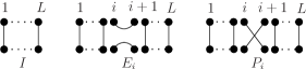
Figure 1: The identity $I$ and the generators $E_{i},P_{i}$ of the Brauer algebra of dimension $(2L-1)!!$ are represented on the left; the walled Brauer algebra generator $P_{i,i+2}=P_{i}P_{i+1}P_{i}$ is represented on the right.

In order to multiply the diagrams one arranges the first $2L$ vertices horizontally with the remaining $2L$ vertices on top of the first ones. The product of a diagram $d_{1}$ with a diagram $d_{2}$ is the diagram $d_{1}d_{2}$ obtained by i) placing the diagram $d_{1}$ on top of the diagram $d_{2}$, ii) identifying the top of the diagram $d_{2}$ with the bottom of the diagram $d_{1}$ and iii) replacing every loop generated in this process by 0. The periodic Brauer algebra is an extension of the Brauer algebra by two generators $E_{2L}$ and $P_{2L}$ which satisfy the same defining relation as the generators of the Brauer algebra if the index $i\equiv i+2L$ is regarded as periodic. The words of the periodic Brauer algebra are diagrams with the top and the bottom being circles wrapped around a cylinder and carrying $2L$ vertices each, such that the latter are pairwise connected in all possible ways by $2L$ edges living on the surface of the cylinder. The periodic Brauer algebra has infinite dimension.

The elements $E_{i}$ and $P_{i,i+2}=P_{i}P_{i+1}P_{i}$ freely generate a subalgebra called the walled Brauer algebra. The generators $P_{i,i+2}$ are represented on the right in fig. 1. This walled Brauer algebra is of central importance for the study of $\operatorname{u}(S|S)$-invariants as explained in the following. Let $V$ denote the fundamental representation of $\operatorname{u}(S|S)$ and $V^{\star}$ be its dual. Generalizing the well known statement for $\operatorname{u}(N)$, Sergeev proved [40] that there is a surjective homomorphism from the walled Brauer algebra to the invariants of the tensor module $(V\otimes~{}V^{\star})^{\otimes 2L}$ or, equivalently, to the $\operatorname{u}(S|S)$-centralizer of $(V\otimes~{}V^{\star})^{\otimes L}$. This means that the $\operatorname{u}(S|S)$-centralizer of $(V\otimes~{}V^{\star})^{\otimes L}$ can be viewed as some representation of the walled Brauer algebra. In particular, the most general $\operatorname{u}(S|S)$-symmetric spin chain Hamiltonian $H$ one can write down must represent some element of the walled Brauer algebra. If we restrict to nearest neighbor interactions only (hence defining a $\operatorname{u}(S|S)$ version of the Heisenberg chain), we get a Hamiltonian of the form

$$H_{\mathrm{TL}}\ =\ -\sum_{i}t_{i}E_{i}\ .$$ (5.1)

This Hamiltonian, all of its powers and the corresponding evolution operator $e^{-\tau H_{\mathrm{TL}}}$ lie entirely in the Temperley-Lieb subalgebra of the walled Brauer algebra. Thus, by the double centralizer theorem, the symmetry of $H_{\mathrm{TL}}$ must be bigger then $\operatorname{u}(S|S)$. One can show [41] that the spectrum of low lying excitation of the homogeneous chain $H_{\mathrm{TL}}$ in the scaling limit is described by the free field theory of a pair of free symplectic fermions,

$$S\ \sim\ \int d^{2}z\,\partial_{\mu}\eta_{1}(z,\bar{z})\partial^{\mu}\eta_{2}(z,\bar{z}).$$ (5.2)

The degeneracies of the excitations of the lattice model must be computed by employing independent representation theoretic tools developed in [37].

We are naturally interested in deformations of the Temperley-Lieb Hamiltonian (5.1) which break the symmetry all the way down to $\operatorname{u}(S|S)$ and preserve conformal invariance in the continuum limit. The simplest $\operatorname{u}(S|S)$-symmetric Hamiltonian is the sum of generators of the walled Brauer algebra. Since the generator $P_{i,i+2}$ corresponds to second nearest neighbor interactions on the spin chain $(V\otimes~{}V^{\star})^{\otimes L}$, it is natural to consider the following $\operatorname{u}(S|S)$-symmetric deformation of the Hamiltonian (5.1)

$$H_{\text{gen}}\ =\ -\sum_{i}\,\big{[}t_{i}E_{i}+w_{i}P_{i,i+2}+a_{i}E_{i}E_{i+1}+b_{i}E_{i+1}E_{i}\big{]}\ .$$ (5.3)

The eigenvalues of the Hamiltonian (5.3) are more easily computed by working in the adjoint - that is in the diagrammatic - representation of the walled Brauer algebra, rather than in the representation on $(V\otimes~{}V^{\star})^{\otimes L}$. However, when switching between the alternating spin chain and adjoint representations of the walled Brauer algebra one looses control of the degeneracies of eigenvalues. These can be recovered from representation theory by methods similar to those used in [2]. We shall call the Hamiltonian (5.3) algebraic when it is considered in the adjoint representation of the walled Brauer algebra. The actual spectrum of the $\operatorname{u}(S|S)$ alternating spin chain will be a subset of the spectrum of the algebraic Hamiltonian (5.3). We call this subset a $\operatorname{u}(S|S)$-sector of the algebraic Hamiltonian. With a little bit of representation theory of the walled Brauer algebra one can prove that the eigenvalues of the $\operatorname{u}(S-1|S-1)$ spin chain Hamiltonian are a subset of the eigenvalues of the $\operatorname{u}(S|S)$ spin chain Hamiltonian. This is done in essentially the same way as in [2].

At a critical point, the space of states of the statistical model usually possesses some additional discrete symmetries. Without loss of generality one can impose these discrete symmetries on the Hamiltonian (5.3), thereby reducing the number of independent couplings $t_{i},w_{i},a_{i},b_{i}$. The scale invariant vacuum in periodic boundary conditions is necessarily translation invariant. Consequently, we shall restrict to homogeneous Hamiltonians (5.3), i.e. to Hamiltonians that are invariant under the discrete shift automorphism

$$E_{i}\rightarrow E_{i+1},\quad P_{i-1,i+1}\rightarrow P_{i,i+2}$$

of the periodic walled Brauer algebra. If we additionally assume invariance with respect to the reflection automorphism

$$E_{i}\rightarrow E_{2L-i+1},\qquad P_{i,i+2}\rightarrow P_{2L-i,2L-i+2},$$

then the Hamiltonian becomes

$$H\ =\ -\sum_{i=1}^{2L}\,\big{[}tE_{i}+wP_{i,i+2}+a(E_{i}E_{i+1}+E_{i+1}E_{i})\big{]}\ .$$ (5.4)

We shall restrict to real couplings $t,w$ and $a$. It will take some more discussion to gain sufficient intuition into the new couplings $w$ and $a$. In particular we shall argue that $w$ is an exactly marginal coupling which corresponds to the radius parameter $R$ of the continuum theory. The coupling $a$, on the other hand, seems to have little effect and will eventually be set to zero.

In order to interpret the couplings $a$ and $w$ we shall mostly work with the $\operatorname{u}(1|1)$ subsector, i.e. we will consider the Hamiltonian (5.4) as an operator on the state space of the $\operatorname{u}(1|1)$ alternating spin chain. The resulting theory is a discrete version of the free theory of symplectic fermions. We can make the link by introducing a set of $2L$ creation and annihilation fermionic operators

$$\{\varphi_{i},\bar{\varphi}_{j}\}\ =\ \delta_{ij},\qquad i,j=1,\dots,2L\ .$$ (5.5)

These may be employed to represent the generators of the walled Brauer algebra through the following quadratic expressions

$$E_{j} =\ (-1)^{j}(\bar{\varphi}_{j}-\bar{\varphi}_{j+1})(\varphi_{j}+\varphi_{j+1})$$ (5.6)

$$P_{j-1,j+1} =\ (-1)^{j}\big{[}1-(\bar{\varphi}_{j-1}-\bar{\varphi}_{j+1})(\varphi_{j-1}-\varphi_{j+1})\big{]}\ .$$

The continuum limit of the $\operatorname{u}(1|1)$ Hamiltonian (5.4) with $a=0$ is described by an action of the type (5.2), the same we found for $w=0$. In other words, when $a=0$ and $S=1$, the perturbation with $P_{i,i+2}$ is truly redundant: On the lattice, its only effect is to renormalize the sound velocity

$$v_{\text{sound}}\ =\ 2t\sqrt{1+4w}\ .$$

Switching on the coupling $a\neq 0$ in the $\operatorname{u}(1|1)$ alternating spin chain (5.4) provides a quartic interaction in terms of the discrete fermions (5.5). The resulting model does not seem to be exactly solvable. One of the fourth order terms of the continuum theory,

$$\delta S\sim\int d^{2}z\,\eta_{1}(z)\eta_{2}(z)\partial_{\mu}\eta_{1}(z)\partial_{\mu}\eta_{2}(z),$$

has been studied in detail in [42]. It was shown to be either marginally relevant or marginally irrelevant, depending on the sign of its coupling. In the continuum theory, adding a fourth order term in the fermions is actually inconsistent with the $\operatorname{u}(1|1)$ symmetry of the model. Free symplectic fermions possess 16 bulk fields of weight $h=\bar{h}=1$. These are obtained by multiplying $1,\eta_{1},\eta_{2},\eta_{1}\eta_{2}$ with $\partial\eta_{1}$ or $\partial\eta_{2}$ and a similar term with $\bar{\partial}$ in place of $\partial$. Under the right (or left) action of $\operatorname{u}(1|1)$, these transform in four indecomposable projectives. A closer look reveals that only two of the 16 fields are true invariants, i.e. they are annihilated by all the $\operatorname{u}(1|1)$ generators. These two fields are quadratic in the fermions. Hence, adding a fourth order term to the symplectic fermion model breaks the $\operatorname{u}(1|1)$ symmetry. We thus conclude that non-zero values of the parameter $a$ in the lattice theory will not effect the continuum theory, at least not for small enough value of $a$.

We suggest that the above conclusions should essentially remain correct for $S>1$. Numerical diagonalization of the algebraic Hamiltonian (5.4) for $a=0$ indicates that its lowest eigenvalue lies in the $\operatorname{u}(1|1)$-sector. This means that one can compute this lowest eigenvalue by restricting the algebraic Hamiltonian (5.4) to the state space of the $\operatorname{u}(1|1)$ alternating spin chain. Hence, $w$ should be exactly marginal even for $S>1$, at least as long as $a=0$. It is tempting to think that this conclusion remains valid for nonzero values of $a$ and that $a$ continues to be irrelevant.

To have a complete correspondence between the couplings of the $\text{$\mathbb{CP}$}^{S-1|S}$ sigma model and those of our lattice model we are still left with the problem to identify a second lattice coupling that could implement the $\theta$ angle. Let us anticipate that the $\theta$ parameter corresponds to staggering the couplings of the lattice model. We will get back to this in the conclusion.

In the following we shall provide strong evidence for our claim that the spectrum of low lying excitations of the alternating $\operatorname{u}(S|S)$ spin chain (5.4) with $a=0$ is described by the sigma model on the complex projective superspace $\text{$\mathbb{CP}$}^{S-1|S}$ with $\theta=\pi$.

6 Open alternating $\operatorname{u}(S|S)$ spin chain

Following the outcome of our discussion in the last section, let us now work with the alternating $\operatorname{u}(S|S)$-spin chain on the space $(V\otimes~{}V^{\star})^{\otimes L}$ with Hamiltonian

$$H\ =\ -\sum_{i=1}^{2L-1}E_{i}-w\sum_{i=1}^{2L-2}P_{i,i+2}\ .$$ (6.1)

In order to compare numerical results with the continuum theory, we need to consider an open chain. Numerical evidence suggests that in the limit $w\to\infty$ and $L\to\infty$, the eigenvalues $E_{h}(L)$ of the Hamiltonian (6.1) become infinitely degenerated. Therefore, we identify the point $w=\infty$ with the large volume limit of the sigma model on the complex projective superspace $\text{$\mathbb{CP}$}^{S-1|S}$. A similar identification has been proposed in [2] for the $\operatorname{osp}(2S+2|2S)$-spin chain on $V^{\otimes L}$.

Without any additional algebraic guidance, the spectrum of the Hamiltonian (6.1) is rather difficult to analyze. In order to unravel some of the structure, it is useful to classify eigenvalues according to the representations of the walled Brauer algebra that appear in the decomposition of the state space $(V\otimes~{}V^{\star})^{\otimes L}$. If one is interested in states that transform according to some irreducible representation of the $\operatorname{u}(S|S)$ symmetry, it pays off to identify those representations of the walled Brauer algebra that are compatible with the required symmetry. The Hamiltonian (6.1) may then be restricted and diagonalized within each such building block.

We shall be mainly concerned with the numerical analysis of excitations of $H$ whose eigenvalues vanish in the limit $w\to\infty$. On the sigma model side, these are the scaling dimensions of tachyonic fields, i.e. of those fields that can be built from square integrable functions on the complex projective superspace $\text{$\mathbb{CP}$}^{S-1|S}$. According to the results of [43] (see also part I of this work), the space of tachyonic fields may be identified with the multiplicity free direct sum of supersymmetric, self-dual, traceless $\operatorname{u}(S|S)$ tensors $t(k,k)$ of rank $2k>2$ and the indecomposable traceless but reducible tensor $t(1,1)=V\otimes~{}V^{\star}$. Note that the trivial tensor $t(0,0)$ is a submodule of $V\otimes~{}V^{\star}$. In our analysis of the $\text{$\mathbb{CP}$}^{1|2}$ model, these were denoted by $t(k,k)=\Lambda_{k,0}$ for $k\geq 2$. The space $t(1,1)$ contains $\Lambda_{1,0}$ and the trivial module $\Lambda_{0,0}$ twice. More details on these labels can be found in appendix B.

We now restrict the Hamiltonian (6.1) to the submodule of $(V\otimes~{}V^{\star})^{\otimes L}$ that contains all states in the $\operatorname{u}(S|S)$ representations $t(k,k)$, where $k=0,\dots,L$. The vector space of all possible embeddings of $\operatorname{u}(S|S)$ tensors $t(k,k)$ into $(V\otimes~{}V^{\star})^{\otimes L},k\neq 1,$ can be endowed with an action of the walled Brauer algebra and it provides an (indecomposable) representation which we denote by $T_{L,L}(k,k)$. Similarly, the vector space of all possible embeddings of the $\operatorname{u}(S|S)$ tensor $t(1,1)=V\otimes~{}V^{\star}$ into $(V\otimes~{}V^{\star})^{\otimes L}$ can be endowed with an action of the walled Brauer algebra. In this case, the space gives rise to an indecomposable representation $I_{L,L}$. It is not difficult to see that the space $T_{L,L}(0,0)$ (which we defined previously) is a submodule of $I_{L,L}$. The corresponding quotient will be denoted by $T_{L,L}(1,1)=I_{L,L}/T_{L,L}(0,0)$. The space $T_{L,L}(1,1)$ is actually not irreducible either. In fact, it can be shown to possess the module $T_{L,L}(0,0)$ as a quotient. All these statements may be proved using the geometric (adjoint) representation of the walled Brauer algebra.

Borrowing from the literature on self-avoiding walks, we shall call the lowest eigenvalue of the Hamiltonian (6.1) in the space $T_{L,L}(k,k)$ the $2k$-legged water melon exponent $h_{0,0}(k)$. According to our discussion above, the degeneracy of $h_{0,0}(k)$ is $\dim t(k,k)$. The numerical results presented in fig. 2 strongly suggest that the continuum limit of the watermelon exponents is given by the very simple expression

$$h_{0,0}(k)\ =\ \frac{g_{0,0}(w)\operatorname{Cas}(k)}{4}\ =\ \frac{g_{0,0}(w)k(k-1)}{2}\ ,$$ (6.2)

where $\operatorname{Cas}(k)$ is the value of the quadratic Casimir in the irreducible representations $t(k,k)$ for $k\neq 1$. For $k=1$, $\operatorname{Cas}(k)=0$ is the value of the quadratic Casimir in either the adjoint or the trivial representation of $\operatorname{u}(S|S)$. The degeneracy of the $h_{0,0}(1)$ watermelon exponent with the vacuum is due to the fact that, as we mentioned above, $T_{L,L}(0,0)$ is a quotient of $T_{L,L}(1,1)$.

Figure 2: Plot of $g_{0,0}(w)$ extracted from the watermelon exponents $h_{0,0}(2)$, $h_{0,0}(3)$ and $h_{0,0}(4)$ computed at $L=9$ with the help of eq. (6.2).

The numerical results should be compared with our formulas (4.22) and (4.26) that determine the conformal weight $h=\delta C^{(2)}g_{0,0}/4$ of boundary fields in the continuum model. Using the association of the $k^{\text{th}}$ watermelon exponent with the weight $\Lambda_{k,0}$ and the dictionary at the end of appendix B, we conclude that

$$\delta_{0}C^{(2)}([k-1,0,2,0])\ =\ 2k(k-1)\ \ .$$

This is in perfect agreement with our continuum theory. Note that both on the lattice and in the continuum the ratio between the conformal weight and the value of the Casimir element is universal, i.e. it is independent of $k$. On the lattice, the universal function $g_{0,0}=g_{0,0}(w)$ depends on the lattice coupling $w$. The corresponding function $g_{0,0}=g_{0,0}(g_{\sigma},\theta)$ is known explicitly, see eq. (4.26). Anticipating that $\theta=\pi$ in the continuum limit of our lattice theory (see below), we can use the identification $g_{0,0}(w)=g_{0,0}(g_{\sigma},\theta=\pi)$ to determine the functional dependence $w=w(g_{\sigma})$ of the lattice on the sigma model coupling $g_{\sigma}$.

7 Twisted open alternating $\operatorname{u}(S|S)$ spin chains

The numerical analysis performed in the previous section suggests that the spectrum of the open $\operatorname{u}(S|S)$ spin chain is described in the continuum limit by the sigma model on $\text{$\mathbb{CP}$}^{S-1|S}$ subject to Neumann boundary conditions or modified Neumann boundary conditions in the presence of a $\theta$-term. However, the sigma model on $\text{$\mathbb{CP}$}^{S-1|S}$ admits a much larger set of boundary conditions that do not break the global $\operatorname{u}(S|S)$ symmetry, namely those described by the nontrivial complex line bundles over $\text{$\mathbb{CP}$}^{S-1|S}$. The complex line bundles can be different at the different ends of the string and we label them by two integers $M$ and $N$ called monopole charges. These bundles may be introduced by adding boundary terms to the action, that is integrals of locally defined 1-forms along the two boundaries. Each of these forms is then interpreted as a connection defining a complex line bundle. Naturally, if the two bundles are different, then so are the boundary conditions at the two boundaries of the world-sheet. Twisting of the spectrum should then be expected when $M\neq N$. In fact, as we showed in sec. 4.2, the $\operatorname{u}(1|1)$ subsector of the $\text{$\mathbb{CP}$}^{S-1|S}$ sigma model is described by a pair of twisted free symplectic fermions with twisting parameter

$$\tan\pi\lambda_{M,N}=\frac{2lg_{\sigma}^{2}}{1+\Theta_{1}\Theta_{2}g_{\sigma}^{4}},$$ (7.1)

where $\Theta_{1}=\tfrac{\theta}{\pi}+2M$, $\Theta_{2}=\tfrac{\theta}{\pi}+2N$ and $l=M-N$. It is natural to ask if one can associate a spin chain to each of these more general boundary conditions. As we explain in the following, this is indeed possible. We shall describe the general setup in the following subsection. Then we describe our numerical results, first for the $\operatorname{u}(1|1)$ subsector and then for the watermelon exponents in the general twisted open chain.

7.1 Monopole boundary conditions

The space of sections in the non-trivial complex line bundles over $\text{$\mathbb{CP}$}^{S-1|S}$ is endowed with an action of $\operatorname{u}(S|S)$ rather than $\operatorname{psl}(S|S)$. Therefore, in order to break the $\operatorname{psl}(S|S)$ symmetry one can proceed by considering the chain of sec. 6 with some extra $V$’s or some extra $V^{\star}$ attached to the ends of the chain. Depending on what we attach to either end of the chain, there are four cases to consider. We list them in the following together with the Hamiltonians we chose to describe their dynamics

$$\begin{array}[]{rlll}V^{\otimes m}&\!\!\otimes\,(V\otimes V^{\star})^{\otimes L}\otimes\ (V^{\star})^{\otimes n}:&H^{VV^{\star}}&=\ H^{V}_{L}+H_{B}+H^{V^{\star}}_{R}\\[5.69054pt] V^{\otimes m}&\!\!\otimes\,(V\otimes V^{\star})^{\otimes L}\otimes\ V^{\otimes n}:&H^{VV}&=\ H^{V}_{L}+H_{B}+H^{V}_{R}\\[5.69054pt] (V^{\star})^{\otimes m}&\!\!\otimes\,(V\otimes V^{\star})^{\otimes L}\otimes\ (V^{\star})^{\otimes n}:&H^{V^{\star}V^{\star}}&=\ H^{V^{\star}}_{L}+H_{B}+H^{V^{\star}}_{R}\\[5.69054pt] (V^{\star})^{\otimes m}&\!\!\otimes\,(V\otimes V^{\star})^{\otimes L}\otimes\ V^{\otimes n}:&H^{V^{\star}V}&=\ H^{V^{\star}}_{L}+H_{B}+H^{V}_{R},\end{array}$$ (7.2)

where the bulk Hamiltonian is the same as in sec. 6 with $a=0$, i.e.

$$H_{B}\ =\ -\sum_{i=m+1}^{2L+m-1}E_{i}-w\sum_{i=m+1}^{2L+m-2}P_{i,i+2}\ ,$$ (7.3)

while the boundary Hamiltonians are as follows

$$H^{V}_{L}\ = -u\sum_{i=1}^{m}P_{i,i+1}\quad\quad\quad\quad\quad H^{V^{\star}}_{R}\ =\ -v\sum_{i=2L+m}^{2L+m+n-1}P_{i,i+1}$$ (7.4)

$$H^{V^{\star}}_{L}\ = -u\sum_{i=1}^{m-1}P_{i,i+1}-w^{\prime}P_{m,m+2}-t^{\prime}E_{m}$$ (7.5)

$$H^{V}_{R}\ = -t^{\prime\prime}E_{2L+m}-w^{\prime\prime}P_{2L+m-1,2L+m+1}-v\sum_{i=2L+m+1}^{2L+m+n-1}P_{i,i+1}\ .$$ (7.6)

Taking into account that the monopole charges $M$ and $N$ describing the boundary conditions of the $\text{$\mathbb{CP}$}^{S-1|S}$ sigma model can be both positive and negative, the existence of four types of chains (7.2) labelled by two positive integers $m,n$ is quite suggestive of a possible identification. On the other hand, the boundary conditions in the $\text{$\mathbb{CP}$}^{S-1|S}$ sigma model and the bundles associated to the corresponding branes do not depend on the details of the connection, but only on their curvature. The latter is essentially fixed by the monopole charge $M$ or $N$. In view of the relation we are about to establish between the spectrum of the $\text{$\mathbb{CP}$}^{S-1|S}$ sigma model and that of the chains (7.2), the previous remarks raise the question as to how much the spectrum of the Hamiltonians (7.2) depend on the precise form of the boundary terms (7.4–7.5). We shall analyze this issue in the $\operatorname{u}(1|1)$ subsector first.

7.2 Numerics for the $\operatorname{u}(1|1)$ subsector

To answer the question of universality and check the applicability of formula (7.1) to the chains (7.2), we first look at their $\operatorname{u}(1|1)$ subsectors. In this subsector, we can extend our representation (5.5) through discrete free fermions to twisted open spin chain. With the boundary interaction terms

$$P_{V\otimes~{}V} =\ -P_{V^{\star}\otimes~{}V^{\star}}\ =\ [1-(\bar{\varphi}_{1}-\bar{\varphi}_{2})(\varphi_{1}-\varphi_{2})]$$

$$P_{V\otimes~{}V^{\star}\otimes~{}V} =\ -P_{V^{\star}\otimes V\otimes~{}V^{\star}}\ =\ [1-(\bar{\varphi}_{1}-\bar{\varphi}_{3})(\varphi_{1}-\varphi_{3})]$$

$$E_{V\otimes V^{\star}} =\ -E_{V^{\star}\otimes V}\ =\ -(\bar{\varphi}_{1}-\bar{\varphi}_{2})(\varphi_{1}+\varphi_{2}),$$

we obtain a free system that can be studied numerically and with great efficiency. Let us anticipate the following three basic outcomes of the numerical analysis.

1. The $\operatorname{u}(1|1)$ spin chains (7.2) flow to the free field theory of symplectic fermions with twisted boundary conditions of the form (2.19).

2. The twisting parameter $\lambda$ does not depend on the boundary couplings $u,t^{\prime},w^{\prime},t^{\prime\prime}$, $w^{\prime\prime},v$ as long as $t^{\prime},t^{\prime\prime},u$ and $v$ are non-zero and the bulk length $L$ of the chain is sufficiently large.

3. In the continuum limit, the dependence of the twisting parameter $\lambda$ on $m,\,n$ and $w$ for all four chains (7.2) is reproduced by eq. (4.23) for the $\text{$\mathbb{CP}$}^{S-1|S}$ sigma model with

   $$\theta=\pi\$$ (7.7)

   provided the following identification between the monopole charges and the thickness of the boundaries of the chains is performed

   $$V^{\otimes m}\otimes(V\otimes V^{\star})^{\otimes L}\otimes(V^{\star})^{\otimes n}: M\ =\ +m\quad N\ =\ +n$$ (7.8)

   $$V^{\otimes m}\otimes(V\otimes V^{\star})^{\otimes L}\otimes V^{\otimes n}: M\ =\ +m\quad N\ =\ -n$$ (7.9)

   $$(V^{\star})^{\otimes m}\otimes(V\otimes V^{\star})^{\otimes L}\otimes(V^{\star})^{\otimes n}: M\ =\ -m\quad N\ =\ +n$$ (7.10)

   $$(V^{\star})^{\otimes m}\otimes(V\otimes V^{\star})^{\otimes L}\otimes V^{\otimes n}: M\ =\ -m\quad N\ =\ -n\,.$$ (7.11)

We now present the numerical evidence supporting these claims one by one.

The numerical calculations supporting claim 1) are presented in fig. 3, where we compare the conformal dimension $h$ for the ground state of our spin chain with the expression

$$h\ =\ \frac{\lambda(\lambda-1)}{2}\ \$$ (7.12)

which determined the conformal dimension of twist fields in terms of the twist parameter $\lambda$. For the lattice model, the twist parameter is measured as the first excitation over the vacuum in the $\operatorname{u}(1|1)$ subsector.

Figure 3: Conformal dimension of the ground state of one of the chains (7.2) compared to the prediction provided by a twisted spectrum.

Numerical evidence for the claim 2. on universality in the choice of the boundary terms (7.4–7.5) is presented in fig. 4.

Figure 4: Universality of $\lambda_{M,N}$ for several chains at $w=0$ and $w=4$.

Combining our claims 1. and 2. we see that for generic boundary couplings $u,t^{\prime},w^{\prime},t^{\prime\prime},w^{\prime\prime},v$ the spectrum of the Hamiltonian (7.2), or at least of their $\operatorname{u}(1|1)$ subsectors, depend only on the thickness $m$ and $n$ of the boundaries. In conclusion, the number of relevant parameters in the four boundary terms (7.4–7.5) exactly matches the number of parameters for the set of boundary conditions preserving the global symmetry of the $\text{$\mathbb{CP}$}^{S-1|S}$ sigma model.

Finally, we present in fig. 5 compelling evidence for the last claim 3. Using numerical data for $\lambda_{M,N}$ generated from chains with different values of $M,\,N$ and $w$, we plotted on the same graph $g_{\sigma}^{2}$ expressed as a function of $\tan\pi\lambda_{M,N}$ from eq. (7.1) with $\theta=\pi$. The appearance of a one to one correspondence between $w$ and $g_{\sigma}^{2}$, which is independent of the chain we use, justifies the applicability of eq. (7.1) to the spin chains, the correct value (7.7) of the $\theta$-angle and the correct identification of the monopole charge (7.8–7.11).

This completes our analysis of the $\operatorname{u}(1|1)$ subsector for the chains (7.2). So far, all our numerical results were in perfect agreement with the continuum $\text{$\mathbb{CP}$}^{0|1}$ sigma model. This supports our claim that the alternating $\operatorname{u}(N|N)$ spin chain provides a discretization for the $\text{$\mathbb{CP}$}^{S-1|S}$ sigma model and it gives us sufficient confidence to address the watermelon exponents for twisted spin chains with $S>1$.

Figure 5: Numerical evaluation of the one-to-one correspondence between the $\text{$\mathbb{CP}$}^{S-1|S}$ sigma model coupling constant $g_{\sigma}^{2}$ and the bulk coupling constant $w$ of the spin chains (7.2). For the chains $N=0$ we represent both branches for $g_{\sigma}^{2}$ expressed as a function of $\tan\pi\lambda_{M,N}$. Calculations where made for $L=800$.

7.3 Watermelon exponents for the twisted open chain

Our aim now is to generalize the discussion of section 6 to the case of general monopole boundary conditions. More precisely, we would like to determine the conformal weight of tachyon vertex operators. For $l>0$, the latter are associated with supersymmetric irreducible traceless tensors $t(k+l,k)$ of contravariant rank $k+l$ and covariant rank $k$, while for $l<0$ these are the supersymmetric irreducible traceless tensors $t(k,k+|l|)$ of contravariant rank $k$ and covariant rank $k+|l|$. In both case $k$ is a non-negative integer, which for $\text{$\mathbb{CP}$}^{1|2}$ corresponds to the labels $\Lambda_{k,l}$ used before.

Let us restrict the algebraic Hamiltonians (7.2) to the representation of the walled Brauer algebra provided by the space of embeddings of the tensors $t(k+l,k)$ and $t(k,k+|l|)$ into the spin chains (7.8–7.11) with monopole numbers $M$ and $N$. The lowest eigenvalue of the Hamiltonian in each of these sectors will be called the $(2k+|l|)$-legged watermelon exponent $h_{M,N}(k)$. As in the case of the chain in sec. 6, the watermelon exponents all vanish in the limit $w\rightarrow 0$, i.e. in the region that we associated with the large volume limit of the $\text{$\mathbb{CP}$}^{S-1|S}$ sigma model. The first two of these watermelon exponents are already contained in the $\operatorname{u}(1|1)$ subsector of the model, both in the continuum and on the lattice. They are not degenerate. The exponent $h_{M,N}(0)$ describes the twisted vacuum, while $h_{M,N}(1)$ is associated with the first excitation. Their non-zero difference is

$$\lambda_{M,N}\ =\ h_{M,N}(1)-h_{M,N}(0)\ .$$ (7.13)

Another important observation coming from lattice calculations is the Casimir evolution for the excitations of the spin chains (7.2). Numerical calculations provide compelling evidence that the following formula

$$\delta h_{M,N}(k)\ =\ h_{M,N}(k)-h_{M,N}(0)\ =\ g_{M,N}\frac{k(k+|l|-1)}{2}\$$ (7.14)

holds for sufficiently large $w$ and with a universal function $g_{M,N}$ that depends only on $M,N$ and $w$. In order to compare with our continuum theory, we note that

$$\delta_{l}C^{(2)}\left[\frac{l}{2}+k-1,0,\frac{l}{2}+2,\frac{l}{2}\right]-\delta_{l}C^{(2)}\left[\frac{l}{2},0,\frac{l}{2},\frac{l}{2}\right]\ =\ 2k(k+l-1)\$$ (7.15)

for $l=M-N>0$. A similar result can be obtained when $l=M-N<0$. The expression $\delta_{l}C^{(2)}$ was defined in eq. (4.22). The watermelon exponents $h_{M,N}(k)$ are associated with the label $\Lambda_{k,l}$. The translation into the label used in eq. (4.22) can be found at the end of appendix B. In conclusion, we see that our lattice observation (7.14) for the watermelon exponents agrees with their proposed continuum description in the $\text{$\mathbb{CP}$}^{1|2}$ model.

By analogy with sec. 6, the function $g_{M,N}$ should be interpreted as the effective tension of the string stretching between the bundle with monopole charge $M$ and the bundle with monopole charge $N$. In the continuum theory, we related the function $g_{M,N}$ to the twist parameter $\lambda_{M,N}$ through the equation

$$\lambda_{M,N}\ =\ \frac{|M-N|}{2}g_{M,N}\ .$$ (7.16)

It is interesting to test the validity of this relation numerically. In fig. 6

Figure 6: Test of eq. (7.16) following from the assumption of Casimir evolution (7.14). Calculations where made for spin chains (7.2) of bulk length $L=7$ and $L=8$ and the corresponding curves almost superpose.

we represent the ratio $|l|g_{M,N}/2\lambda_{M,N}$ as a function of $w$. As before, we measure the function $g_{M,N}$ through the equation (7.14) for different excitations $h_{M,N}(k)$. If the Casimir evolution (7.14) holds true, then we should see a constant value of $|l|g_{M,N}/2\lambda_{M,N}=1$ for the ratio, independently of the watermelon exponent that is used to measure $g_{M,N}$. While things work out remarkably well in the regime of large $w$, obvious discrepancies appear when $w$ is close to $w\sim 0$. The possible interpretation of these differences are discussed in the next subsection.

7.4 Comments on the region of small $w$

There are actually several possibilities to interpret the failure of eq. (7.16) near $w=0$. We will discuss two scenarios below. The ultimate test of the correct explanation will be left for future work. In confronting our numerical results with the proposed continuum description, we have tacitly assumed that the spin chains (7.2) at $w=0$ still describe a point in the moduli space of the $\text{$\mathbb{CP}$}^{S-1|S}$ sigma model. This is a very strong assumption given that the symmetry of the bulk Hamiltonian (7.3) becomes much larger [37] than $\operatorname{u}(S|S)$ at $w=0$, essentially because the lines in the Brauer algebra representation are then prevented from crossing.

In assessing the meaning of the observed discrepancies, it is useful to recall that a similar issue has also appeared for the $\operatorname{osp}(2S+2|2S)$ spin chain considered in [2]. The $\operatorname{osp}$ spin chain was proposed as a discretization of the $S^{2S+1|2S}$ supersphere sigma model. Generic features of the lattice spectrum were found to be in excellent agreement with the conjectured spectrum of the sigma model, as long as $w$ was large. However, problems similar to the ones we described in the previous subsection were encountered at the point $w=0$. Note that in the supersphere case, the discrepancy was only visible when looking at fields outside the $\operatorname{O}(2)$ subsector of $\operatorname{osp}(2S+2|2S)$ theory. Again, a very similar observation was made for the $\operatorname{u}(1|1)$ sector of the $\operatorname{u}(S|S)$ spin chain. With all these similarities, it seems likely that the discrepancies between lattice and continuum analysis in the $\operatorname{u}(S|S)$ and osp(2S+2$|$2S) model should have the same explanation.

In the case of the supersphere sigma model, however, the assumption of Casimir evolution for the whole spectrum stands on rather firm grounds. To begin with, the perturbative expansion for boundary conformal weights in the supersphere model may be summed to all orders. Terms that could spoil the Casimir evolution were shown to vanish. Moreover, world-sheet instanton corrections cannot alter these findings, simply because they do not exist in this case. Finally, a conjectured duality between the supersphere sigma model and the osp(2S+2$|$2S) Gross-Neveu model was shown to be perfectly consistent with the Casimir evolution of boundary conformal weights [44, 4]. All this makes it seem very likely that the conformal weights of the two investigated sigma models all evolve with the Casimir, as encoded in our formula (4.2).

Having argued that the discrepancies between our lattice and continuum results are unlikely to signal a breakdown of the Casimir evolution in the sigma model, we want to entertain a second logical possibility, namely that the continuum limit of the spin chains (7.2) is described by a $\text{$\mathbb{CP}$}^{S-1|S}$ sigma model only for $w>0$, while at $w=0$ it is not. If this was true then the discrepancies we observed in fig. 6 would simply result from interchanging the thermodynamic limit $L\to\infty$ with the limit $w\to 0$. A similar non-commutativity of limiting procedures can also be observed in the large volume limit $w\to\infty$ where the symmetry of the Hamiltonian is once more enhanced much beyond the generic $\operatorname{u}(S|S)$ transformations.

Support for our second explanation of the discrepancies comes from a closer inspection of the watermelon exponents. At $w=0$, the lattice model is exactly solvable and we believe that the differences between water-melon exponents are given by

$$\delta h_{M,N}(k)\ =\ \frac{k(k+2\lambda_{M,N}-1)}{2}$$ (7.17)

where $\lambda_{M,N}$ is again measured as the difference $\lambda_{M,N}=h_{M,N}(1)-h_{M,N}(0)$. The formula (7.17) can most certainly be derived analytically. But for now, we simply justify it by observing that it fits the general pattern of boundary exponents in (non intersecting) loop models discussed in [45]. Indeed, it can be rewritten as

$$h_{M,N}(k)\ =\ h_{2\lambda_{M,N}-1,2\lambda_{M,N}-1+2k}$$

where on the right hand side we use the Kac formula at $c=-2$:

$$h_{r,s}=\frac{(2r-s)^{2}-1}{8}$$

A verification of this formula is presented in tab. 7.4. The numbers in the grid should all go to unity in the scaling limit. We see that the agreement with eq. (7.17) is quite impressive. The behavior of watermelon exponents in the chain with $w\neq 0$ is significantly different. This supports our claim that the continuum theory of the $w=0$ lattice model does not belong to the continuous family of conformal field theories that is parametrized by $w>0$.

$M$	$N$	$\tfrac{2\delta h_{M,N}(k)}{k(k+2\lambda_{M,N}-1)}$
		$k=2$	$k=3$	$k=4$
1	0	1.050128	1.037253	1.010766
2	0	1.098296	1.094754	1.070405
0	-1	0.98817	0.969892	0.945022
0	-2	1.016252	1.006706	0.984296
1	-2	1.034566	1.033275

Table 1: Numerical check of the proposed formula (7.17) for the watermelon exponents of the spin chains (7.2) at $w=0$. Calculations where made for bulk length $L=7$.

8 Conclusions and Open Problems

In this work we have analyzed the boundary partition functions for all $\text{u}(2|2)$ invariant boundary conditions of the sigma model in the projective superspace $\text{$\mathbb{CP}$}^{1|2}$. The dependence of this partition function on the bulk couplings $g_{\sigma}$ and $\theta$ and on the boundary monopole charges $M,N$ was displayed in eq. (4.2). It contains the branching functions (3.20) of the model at $R=\infty$ along with two universal functions $\lambda_{M,N}$ and $g_{M,N}$ which are defined through eqs. (4.23) and (4.24), respectively. The partition function encodes the dependence of boundary conformal weights on the various couplings and justifies and generalizes the results in [15]. In the second part, we introduced a lattice model with Hamiltonian (5.4) on an alternating spin chain. Numerical studies of the latter revealed an excellent agreement with the predictions from the continuum theory, at least for sufficiently large values of the lattice coupling $w$. In particular, we were able to model all the boundary conditions of the continuum theory by adding boundary layers of finite width to the open spin chain, see eq. (7.2).

One of the most interesting applications of our results would be to search for values of the parameters $g_{\sigma}$ and $\theta$ at which the world-sheet symmetry gets enhanced, e.g. to some affine Lie algebra symmetry. A similar Wess-Zumino point exists for sigma models on superspheres $S^{2S+1|2S}$ and it gives rise to an interesting dual description of the theory through a non-geometric Gross-Neveu model. It is very likely that similar points exist for sigma model on complex projective superspaces as well. Even though we have not yet been able to identify a point with affine psl(2$|$2) symmetry, we hope to return to this issue soon.

Another possible further direction concerns the closely related non-compact sigma model on the coset space $\text{U}(1,1|2)/\text{U}(1|1)\times\text{U}(1|1)$ that was considered in [14] because of its possible relevance for the theory of quantum Hall plateau transitions. The spin chain discussed in [14] involves infinite dimensional representations and a pure Heisenberg interaction. It would be interesting, among other things, to study the role of next to nearest neighbor interactions in that case, and to analyze whether they allow fine tuning of the running coupling constant as in our model. It could also be of interest to interpret our bundle boundary conditions in terms of edge states in the Hall effect [18].

A striking conclusion of our study is that, like in the supersphere case, the chain with the simplest interaction (no loop crossing in the Brauer formulation, or $w=0$) seems to be in a different universality class from the generic $w\neq 0$ case. Non-commutativity of the limits $L\to\infty$ and $w\to 0$ means more precisely that the perturbation induced by turning $w\neq 0$ on the lattice is relevant at $w=0$. The conformal field theory at that point admits a very large symmetry, but has not yet been fully explored. For the whole picture to be consistent, the bulk spectrum should contain an invariant, marginally relevant operator, which should moreover be absent in the minimal $\text{U}(1\,|1)$ or $\operatorname{O}(2)$ subsector. The existence of this operator remains to be established.

Let us point out that there are some other predictions of the Casimir evolution that could be checked in the large volume regime. Note that the Casimir evolution for the weights of tachyonic vertex operators is supported by both perturbative and non-perturbative numerical calculations only in the theory with equal boundary monopole charges $M=N$. While the conjectured exact form (4.20) of watermelon exponents in the theory with arbitrary boundary monopole charges $M,N$ passed several analytical and numerical tests, it could not be backed up by perturbative calculations beyond the leading order because we did not succeed to generalize the background field expansion to twisted boundary conditions. Nonetheless, we suspect that such a generalization exists and the watermelon exponents will most likely be computed again in terms of eigenvalues of some Laplacian on the bundle with monopole charge $l=M-N$. The point is that for $l\neq 0$ this Laplacian is not unique, as can be seen from the existence of a 1-parameter family of $\operatorname{u}(S|S)$ Casimirs $\operatorname{Cas}_{\alpha}$, see app. B. However, if we choose

$$\alpha=1-\frac{g_{M,N}(g_{\sigma},\theta)}{2}$$

then the conjectured form (4.20) for the watermelon exponents coincides exactly with a Casimir evolution type formula

$$h^{g_{\sigma},\theta}_{M,N}(k)=\frac{g_{M,N}(g_{\sigma},\theta)}{4}\operatorname{Cas}_{\alpha}(\Lambda_{k,l}),$$

which is most natural in the context of the background field method. On the other hand, these conjectured watermelon exponents possess the following simple expansion in the coupling $g_{\sigma}$,

$$h_{M,N}(k)\ =\ \frac{g^{2}_{\sigma}}{\pi}\operatorname{Cas}_{\alpha=1}(\Lambda_{k,l})+\frac{2g_{\sigma}^{4}}{\pi^{2}}l^{2}+O(g_{\sigma}^{6})\ .$$

Here, $\operatorname{Cas}_{\alpha=1}(\Lambda_{k,l})$ are the eigenvalues of the Bochner-Laplacian of the complex line bundles over $\text{$\mathbb{CP}$}^{S-1|S}$ and, as we said, the first term can be reproduced by the semi-classical approximation. In the case $l\neq 0$ the first correction to the semi-classical result comes at order $g_{\sigma}^{4}$. This is an accessible non-trivial check to be performed once the perturbation theory for twisted boundary conditions is ironed out.

Moving away from $\theta=\pi$ in the sigma model corresponds to staggering the couplings of the spin chain. In the case $w=0$, it is well known that staggering in fact does not affect the spectrum at all. For $w\neq 0$, we expect in general that staggering will renormalize the coupling constant to which the lattice model flows (so the $g_{\sigma}^{2}(w)$ dependence will be now a dependence on $w$ and the staggering parameter), on top of affecting the value of $\theta$ in the formulas. Our continuum theory makes rather non-trivial predictions about this functional dependence that seem well worth further investigation.

Acknowledgments: We especially thank N. Read for an earlier collaboration on the subject, and for many illuminating comments and discussions. We thank Nathan Berkovits, Thomas Creutzig, Manfred Herbst, Marcos Marino, Tristan McLoughlin, Nikita Nekrasov, Nick Read, Soo-Jong Rey, Peter Rønne, Sakura Schäfer-Nameki and Edward Witten for discussions and comments. We are gratefull to the Galileo Galilei Institute for its hospitality during the beginning of this work. This research was supported in part by the National Science Foundation under Grant No. PHY05-51164. The research of TQ is funded by a Marie Curie Intra-European Fellowship, contract number MEIF-CT-2007-041765. HS was supported by the ANR and the Network INSTANS.

Appendix A The quadratic Casimir elements

For a simple contragredient Lie superalgebra $\mathfrak{g}$ the invariant, supersymmetric, consistent, non-degenerate and bilinear form $\beta:\mathfrak{g}\times\mathfrak{g}\rightarrow\mathbb{C}$ exists and is defined uniquely up to a proportionality constant. Every such invariant form $\beta$ defines a quadratic central element in the universal enveloping Lie superalgebra in the standard way. To be more precise, let $T_{a}$ be a basis of $\mathfrak{g}$ and let $T^{a}$ be the dual basis with respect to $\beta$, that is

$$\beta(T^{a},T_{b})\ =\ \delta^{a}_{b}.$$ (A.1)

Then the quadratic Casimir associated to the invariant form $\beta$ is defined as

$$\operatorname{Cas}\ =\ \sum_{a}T_{a}T^{a}\ .$$ (A.2)

It is not hard to verify that $\operatorname{Cas}$ is indeed central. The Lie superalgebra $\text{u}(S\,|S)$ we are dealing with in this work, however, is not simple. After a normalization has been fixed, it possesses a one parameter family of invariant, supersymmetric, consistent, non-degenerate and bilinear forms. Let $V\simeq V_{\bar{0}}\oplus V_{\bar{1}}$ denote the graded fundamental module of $\text{u}(S\,|S)$ with even dimension $\dim V_{\bar{0}}=S$ and odd dimension $\dim V_{\bar{1}}=S$ and $R_{V}:\text{u}(S\,|S)\rightarrow\operatorname{u}(V)$ be the corresponding representation. Then the one parameter space of invariant forms of $\text{u}(S\,|S)$ is constructed by using the invariant supertrace

$$\beta(X,Y)\ =\ \operatorname{\text{str}}R_{V}(XY)+\alpha\operatorname{\text{str}}R_{V}(X)\operatorname{\text{str}}R_{V}(Y)\ .$$ (A.3)

Let now $E_{i\phantom{j}}^{\phantom{i}j}$ be the standard basis of $\operatorname{u}(V)$, that is the $2S\times 2S$ matrices with an entry 1 in the $i$-th row and $j$-th column and 0 entries everywhere else. According to the def. (A.1), the basis dual to $E_{i\phantom{j}}^{\phantom{i}j}$ with respect to the form (A.3) is given by

$$\Big{(}E_{i\phantom{j}}^{\phantom{i}j}\Big{)}^{*}\ =\ (-1)^{|j|}E_{j\phantom{i}}^{\phantom{j}i}-\alpha\delta^{i}_{j}E\ ,$$

where we have denoted by $E$ the identity matrix. The quadratic Casimir of a reductive Lie superalgebra is constructed in the same way as in eq. (A.2). When the invariant forms are not unique, the same is true for the Casimir element. In particular, the quadratic Casimir element of $\text{u}(S\,|S)$ that is associated to the form (A.3) becomes

$$\operatorname{Cas}_{\alpha}\ =\ E_{i\phantom{j}}^{\phantom{i}j}E_{j\phantom{i}}^{\phantom{j}i}(-1)^{|j|}-\alpha E^{2}\ .$$ (A.4)

The eigenvalues of $\operatorname{Cas}_{\alpha}$ in an irreducible representation with highest weight $\Lambda$ can be evaluated by computing scalar products in the weight space $\mathfrak{h}^{*}$ in exactly the same way as for simple Lie superalgebras. Let us see how this works. Choose the diagonal generators $D_{1}=E_{1\phantom{1}}^{\phantom{1}1},\dots,D_{2S}=E_{2S\phantom{2S}}^{\phantom{2S}2S}$ as a basis of the Cartan subalgebra $\mathfrak{h}$ of $\text{u}(S\,|S)$ and denote by $\epsilon_{1},\dots,\epsilon_{S},\delta_{1},\dots,\delta_{S}$, respectively, the dual basis in $\mathfrak{h}$. The restriction of $\beta$ to $\mathfrak{h}$ defines a natural isomorphism $\varphi:\mathfrak{h}\rightarrow\mathfrak{h}^{*}$ by

$$\varphi(H^{\prime})(H^{\prime\prime})\ =\ \beta(H^{\prime},H^{\prime\prime})$$ (A.5)

and endows $\mathfrak{h}^{*}$ with a scalar product

$$(\lambda,\mu)_{\alpha}\ =\ \beta\big{(}\varphi^{-1}(\lambda),\varphi^{-1}(\mu)\big{)}\ .$$ (A.6)

In the basis $\delta_{i},\epsilon_{j}$ of $\mathfrak{h}^{*}$, the natural isomorphism (A.5) reduces to

$$\varphi(D_{1})\ =\ \epsilon_{1},\dots,\varphi(D_{2S})\ =\ \delta_{S}.$$

The matrix elements of the scalar product (A.6) in the weight space $\mathfrak{h}^{*}$ of $\text{u}(S\,|S)$ with respect to the basis $\epsilon_{i},\delta_{j}$ can easily be computed

$$(\epsilon_{i},\epsilon_{j})_{\alpha}\ =\ \delta_{ij}-\alpha,\quad(\delta_{i},\delta_{j})_{\alpha}=-\delta_{ij}-\alpha,\quad(\epsilon_{i},\delta_{j})_{\alpha}=-\alpha\ .$$ (A.7)

One natural way to parametrize the highest weight vectors $\Lambda$ for irreducible representations of $\text{u}(S\,|S)$ is by specifying the coordinates of $\Lambda$ with respect to the basis $\epsilon_{i},\delta_{j}$. Thus, if

$$\Lambda\ =\ \sum_{i=1}^{S}\rho_{i}\delta_{i}+\sigma_{i}\epsilon_{i}$$ (A.8)

is the highest weight of a highest weight representation, then

$$\sigma_{i}\ =\ \Lambda(D_{i}),\quad\rho_{i}\ =\ \Lambda(D_{S+i}),\qquad i=1,\dots,S\ .$$ (A.9)

The eigenvalues of the Casimir element do not depend on the conventions for positiveness in the weight space. To compute them, we shall use a non-standard, but convenient absolute ordering

$$\epsilon_{1}\ >\ \dots\ >\ \epsilon_{S}\ >\ \delta_{1}\ >\ \dots\ >\ \delta_{S}$$ (A.10)

which fixes the positive roots to

$$\epsilon_{i}-\epsilon_{j},\quad\delta_{k}-\delta_{l},\quad\epsilon_{i}-\delta_{k}\ ,$$

where $i<j$ and $k<l$. Now if $v_{\Lambda}$ is the highest weight vector of some highest weight representation, then the eigenvalue of the Casimir on that representation can be easily computed

$$\operatorname{Cas}_{\alpha}v_{\Lambda} =\ \sum_{i=1}^{2S}(-1)^{|i|}D_{i}^{2}v_{\Lambda}-\alpha E^{2}v_{\Lambda}+\sum_{j=2}^{2S}\sum_{i=1}^{j-1}[E_{i\phantom{j}}^{\phantom{i}j},E_{j\phantom{i}}^{\phantom{j}i}](-1)^{|j|}v_{\Lambda}$$

$$=\left(\sum_{i=1}^{2S}(-1)^{|i|}\Lambda(D_{i})^{2}-\alpha\Lambda(E)^{2}+\sum_{j=2}^{2S}\sum_{i=1}^{j-1}[(-1)^{|j|}\Lambda(D_{i})-(-1)^{|i|}\Lambda(D_{j})]\right)v_{\Lambda}\ .$$

Using the eqs. (A.7, A.8 and A.9) one can derive the desired form for the eigenvalues $\operatorname{Cas}_{\alpha}(\Lambda)$ of the Casimir (A.4) in a highest weight representation with highest weight $\Lambda$, namely

$$\operatorname{Cas}_{\alpha}(\Lambda)\ =\ (\Lambda,\Lambda+2\rho)_{\alpha},$$ (A.11)

where $\rho$ is the Weyl vector

$$2\rho\ =\ \sum_{1\leq i<j\leq S}(\epsilon_{i}-\epsilon_{j}+\delta_{i}-\delta_{j})-\sum_{i,j=1}^{S}(\epsilon_{i}-\delta_{j})$$

with respect to the chosen absolute ordering (A.10). Keeping in mind that the Weyl vector is the half sum of all positive roots minus the half sum of all negative roots, the formula eq. (A.11) for the eigenvalues of the Casimir can be rendered independent of the definition of positiveness in the weight space.

In the paper we use another notation for the weights of $\text{u}(2|2)$, which stems from a different choice (3.11) of basis for the Cartan algebra. With respect to this basis, a highest weight $\Lambda=[j_{1},j_{2},a,b]$ has the following components

$$\Lambda(J_{x})\ =\ j_{1}\,,\quad\Lambda(J_{y})\ =\ j_{2},\quad\Lambda(J_{z})\ =\ a\,,\quad\Lambda(J_{u})\ =\ b\ .$$ (A.12)

The dictionary between the labels $\rho_{i},\sigma_{j}$ of eq. (A.8) and the labels $j_{1},j_{2},a,b$ is easy to establish

$$\sigma_{1}-\sigma_{2}\ =\ 2j_{1}\,,\quad\rho_{1}-\rho_{2}\ =\ 2j_{2}\,,\quad\sigma_{1}+\sigma_{2}-\rho_{1}-\rho_{2}\ =\ 2a\,,\quad\sigma_{1}+\sigma_{2}+\rho_{1}+\rho_{2}\ =\ 2b\ .$$ (A.13)

Moreover, from eq. (A.11) we obtain our formula (3.17) for the value of the Casimir elements in the representations $[j_{1},j_{2},a,b]$ of $\text{u}(2|2)$.

Appendix B Laplacian on complex line bundles over $\text{$\mathbb{CP}$}^{S-1|S}$

Let $g_{pq}$ be the matrix elements of the metric $g$ on $\text{$\mathbb{CP}$}^{S-1|S}$ in some set of local real coordinates $\varphi^{p}$, $g^{pq}$ be the matrix inverse to $g_{pq}$, $\nabla$ be the Levi-Civita connection with respect to the metric $g$ and $A=A_{p}(\varphi)d\varphi^{p}$ be the one-form monopole defining a complex line bundle over $\text{$\mathbb{CP}$}^{S-1|S}$. Then the Bochner-Laplacian on the complex line bundle over $\text{$\mathbb{CP}$}^{S-1|S}$ is defined by the following second order, $\text{u}(S\,|S)$-invariant differential operator

$$\Delta=g^{pq}(\nabla_{p}+A_{q})(\nabla_{p}+A_{q}).$$

Existence theorems [46] ensure that a non-trivial complex line bundle exists and is unique if and only if the curvature $\Omega=dA$ of the connection $A$ satisfies the following integrality condition

$$\int_{\text{$\mathbb{CP}$}^{1}}\frac{\Omega}{2\pi i}\in\mathbb{Z}.$$

Let $w^{i}$ be a set of local holomorphic coordinates on $\text{$\mathbb{CP}$}^{S-1|S}$. Then the standard metric on $\text{$\mathbb{CP}$}^{S-1|S}$ is given by the Fubini-Study metric

$$g_{i\bar{\jmath}}=\frac{\delta_{ij}}{1+w^{\dagger}\cdot w}-\frac{(-1)^{|j|}w^{\bar{\imath}}w^{j}}{(1+w^{\dagger}\cdot w)^{2}},$$

where the sign conventions for the scalar product in the supereuclidean space $\mathbb{C}^{S-1|S}$ are $w^{\dagger}\cdot w=\delta_{ij}w^{\bar{\jmath}}w^{i}$. The metric form is

$$ds^{2}=g_{pq}d\varphi^{p}d\varphi^{q}=2g_{i\bar{\jmath}}dw^{\bar{\jmath}}dw^{i}$$

and all the geodesics are closed and of fixed length $\sqrt{2}\pi$. The Kähler form

$$\omega=-ig_{i\bar{\jmath}}dw^{\bar{\jmath}}\wedge dw^{i}$$

can be normalized to yield a generator for the second integral cohomology group. Indeed, from

$$\int_{\text{$\mathbb{CP}$}^{1}}\omega=2\pi,$$

the existence condition for the complex line bundle reduces to

$$\Omega=-il\omega,$$

where $l\in\mathbb{Z}$ is called the monopole charge.

By standard methods in the theory of complex line bundles, see [19], one can prove that the space of sections of the bundle with monopole charge $l$ is isomorphic to the space of equivariant functions on $\text{$\mathbb{CP}$}^{S-1|S}$, that is the space of functions $f(w,\bar{w})$ with the property

$$f(e^{i\alpha}w,e^{-i\alpha}\bar{w})=e^{i\alpha l}f(w,\bar{w}),$$

where $\alpha$ is real. This functional space can be constructed as a square integrable span on the monomials $Z^{i_{1}}\dots Z^{i_{k+l}}\bar{Z}^{j_{1}}\dots\bar{Z}^{j_{k}}$, where $Z^{i}$ are the components of some vector belonging to the $\text{u}(S\,|S)$-fundamental representation $\square$ satisfying $Z^{\dagger}\cdot Z=1$ and $k,l$ are integers such that $k\geq 0,\,k+l\geq 0$.

The harmonic decomposition of the space of equivariant functions with monopole charge $l\neq 0$ is a multiplicity free direct sum of $\text{u}(S\,|S)$ supersymmetric traceless irreducible tensors $t(k+l,k)$ of contravariant rank $k+l\geq 0$ and covariant rank $k\geq 0$. The highest weights of these tensors can be easily computed in the $\delta_{i},\epsilon_{j}$ basis of sec. A. If one chooses the absolute ordering (A.10) in the weight space of $\text{u}(S\,|S)$ then the highest weight of the fundamental representation becomes $\epsilon_{1}$, while of that of the dual representation $-\delta_{S}$. The weight of a supersymmetric tensor power of a vector follows immediately from the definition of the tensor action of the superalgebra. Thus, the highest weights of the supersymmetric irreducible traceless tensors $t(k+l,k),\,l>0$ are

$$\Lambda_{k,l}=\begin{cases}(k+l)\epsilon_{1}-\delta_{S-k+1}-\dots-\delta_{S},&k\leq S\\ (k+l)\epsilon_{1}-(k-S)\epsilon_{S}-\delta_{1}-\cdots-\delta_{S},&k>S\end{cases},$$

while those of the tensors $t(k^{\prime}+l,k^{\prime})=t(k,k+|l|),\,l<0$ are

$$\Lambda_{k,l}=\begin{cases}k\epsilon_{1}-\delta_{S-k-|l|+1}-\dots-\delta_{S},&k+|l|\leq S\\ k\epsilon_{1}-(k+|l|-S)\epsilon_{1}-\delta_{1}-\dots-\delta_{S},&k+|l|>S\end{cases},$$

where in both cases $k\geq 0$.

With this explicit construction of the complex line bundles at hand one can compute the spectrum of the Bochner-Laplacian, see  [19]. The net result for the eigenvalues $\lambda_{l}(k)$ of $\Delta$ is

$$\lambda_{l}(k)=-2\left(k+\frac{|l|}{2}\right)\left(k+\frac{|l|}{2}-1\right)+\frac{l^{2}}{2},$$ (B.1)

where $k\geq 0$. Comparing this spectrum to the eigenvalues of the Casimir (A.4, A.11)

$$\operatorname{Cas}_{\alpha}(\Lambda_{k,l})=2k^{2}+(2k+|l|)(|l|-1)-\alpha l^{2},$$ (B.2)

we see that

$$\Delta=-\operatorname{Cas}_{\alpha=1}.$$

In the end let us list the labels (A.12) of the highest weights $\Lambda_{k,l}$ of supersymmetric traceless irreducible $\text{u}(2|2)$-tensors $t(k+l,k)$ and $t(k,k+|l|)$. Using the dictionary (A.13) we get for $l\geq 0$

$$\Lambda_{0,l}=\left[\frac{l}{2},0,\frac{l}{2},\frac{l}{2}\right],\quad\Lambda_{1,l}=\left[\frac{l+1}{2},\frac{1}{2},\frac{l}{2}+1,\frac{l}{2}\right],\quad\Lambda_{k,l}=\left[\frac{l}{2}+k-1,0,\frac{l}{2}+2,\frac{l}{2}\right],$$

for $k=2,3,\dots$. When $l<0$ we have

$$\Lambda_{0,-1}=\left[0,\frac{1}{2},\frac{1}{2},-\frac{1}{2}\right],\quad\Lambda_{k,l}=\left[-\frac{l}{2}+k-1,0,\frac{l}{2}+2,\frac{l}{2}\right],\quad k+|l|\geq 2.$$

Appendix C Atypical branching functions

In this appendix we collect explicit formulas for the branching functions of atypical $\text{u}(2|2)$ representations in terms of those for Kac-modules. Let latter were displayed in the main text. As in the rest of the paper, finite dimensional representations of $\text{u}(2|2)$ are labelled by four parameters $j_{1},j_{2}\in\mathbb{N}/2$ and $a,b\in\mathbb{R}$. There are five different kinds of atypicality conditions on these labels. For each of these we shall then list the atypical branching functions. All of them can be derived using the character formulas in [21].

• $b=j_{1}-j_{2}=0$

  $$\psi_{[0,0,a,0]} = \psi_{[0,0,a,0]}^{K}+\psi_{[0,0,a+4,0]}^{K}+\psi_{\left[\frac{1}{2},\frac{1}{2},a+1,0\right]}^{K}+\psi_{\left[\frac{1}{2},\frac{1}{2},a+3,0\right]}^{K}$$

  $$\psi_{\left[\frac{1}{2},\frac{1}{2},a,0\right]} = \psi_{\left[\frac{1}{2},\frac{1}{2},a,0\right]}^{K}+\psi_{\left[\frac{1}{2},\frac{1}{2},a+2,0\right]}^{K}+\psi_{[0,0,a+1,0]}^{K}+\psi_{[1,1,a+1,0]}^{K}$$ (C.1)

  $$\psi_{[j,j,a,0]} = \psi_{[j,j,a,0]}^{K}+\psi_{[j,j,a+2,0]}^{K}+\psi_{\left[j-\frac{1}{2},j-\frac{1}{2},a+1,0\right]}^{K}+\psi_{\left[j+\frac{1}{2},j+\frac{1}{2},a+1,0\right]}^{K}\text{ for }j\geq 1$$

• $b=j_{1}-j_{2}\neq 0$

  $$\psi_{\left[\frac{1}{2},0,a,\frac{1}{2}\right]} = \psi^{K}_{\left[\frac{1}{2},0,a,\frac{1}{2}\right]}+\psi^{K}_{\left[0,\frac{1}{2},a+3,\frac{1}{2}\right]}$$

  $$\psi_{\left[0,\frac{1}{2},a,-\frac{1}{2}\right]} = \psi^{K}_{\left[0,\frac{1}{2},0,a,-\frac{1}{2}\right]}+\psi^{K}_{\left[\frac{1}{2},0,a+3,-\frac{1}{2}\right]}$$

  $$\psi_{\left[j_{1},0,a,j_{1}\right]} = \psi^{K}_{\left[j_{1},0,a,j_{1}\right]}+\psi^{K}_{\left[j_{1}-1,0,a+2,j_{1}\right]}\text{ for }j_{1}\geq 1$$ (C.2)

  $$\psi_{\left[0,j_{2},a,-j_{2}\right]} = \psi^{K}_{\left[0,j_{2},a,-j_{2}\right]}+\psi^{K}_{\left[0,j_{2}-1,a+2,-j_{2}\right]}\text{ for }j_{2}\geq 1$$

  $$\psi_{\left[j_{1},j_{2},a,j_{1}-j_{2}\right]} = \psi^{K}_{\left[j_{1},j_{2},a,j_{1}-j_{2}\right]}+\psi^{K}_{\left[j_{1}-\frac{1}{2},j_{2}-\frac{1}{2},a+1,j_{1}-j_{2}\right]}\text{ for }j_{1}\text{ and }j_{2}\geq 0$$

• $b=-j_{1}+j_{2}\neq 0$

  $$\psi_{\left[j_{1},j_{2},a,-j_{1}+j_{2}\right]} = \psi^{K}_{\left[j_{1},j_{2},a,-j_{1}+j_{2}\right]}+\psi^{K}_{\left[j_{1}+\frac{1}{2},j_{2}+\frac{1}{2},a+1,-j_{1}+j_{2}\right]}$$ (C.3)

• $b=j_{1}+j_{2}+1$

  $$\psi_{\left[0,j_{2},a,j_{2}+1\right]} = \psi^{K}_{\left[0,j_{2},a,j_{2}+1\right]}+\psi^{K}_{\left[0,j_{2}+1,a+2,j_{2}+1\right]}$$ (C.4)

  $$\psi_{\left[j_{1},j_{2},a,j_{1}+j_{2}+1\right]} = \psi^{K}_{\left[j_{1},j_{2},a,j_{1}+j_{2}+1\right]}+\psi^{K}_{\left[j_{1}-\frac{1}{2},j_{2}+\frac{1}{2},a+1,j_{1}+j_{2}+1\right]}\text{ for }j_{1}\geq\frac{1}{2}$$

• $b=-j_{1}-j_{2}-1$

  $$\psi_{\left[j_{1},0,a,-j_{1}-1\right]} = \psi^{K}_{\left[j_{1},0,a,-j_{1}-1\right]}+\psi^{K}_{\left[j_{1}-1,0,a+2,-j_{1}-1\right]}$$ (C.5)

  $$\psi_{\left[j_{1},j_{2},a,-j_{1}-j_{2}-1\right]} = \psi^{K}_{\left[j_{1},j_{2},a,-j_{1}-j_{2}-1\right]}+\psi^{K}_{\left[j_{1}+\frac{1}{2},j_{2}-\frac{1}{2},a+1,-j_{1}-j_{2}-1\right]}\text{ for }j_{2}\geq\frac{1}{2}$$

Explicit expressions for the atypical branching functions are now obtained by plugging in our formula (3.20) for the branching functions of Kac modules. The coefficients of atypical branching functions turn out to be positive.

Appendix D Vanishing invariants on $\text{$\mathbb{CP}$}^{S-1|S}$

We start by considering a general symmetric superspace $G/H$, where $G$ is a Lie supergroup with an involutive automorphism $\sigma$ such that $H$ is the maximal compact subgroup of $G$ fixed by $\sigma$. Let $e$ be the identity of $G$ and consider the point $o=eH$. The Riemann structure on $G/H$ is defined by the requirement that $G$ is a supergroup of isometries. This means that the action of $G$ defines the metric and the curvature tensor globally once their values are given at a single point, say $o$.

Let now $\mathfrak{g}$ and $\mathfrak{h}$ denote the Lie superalgebras of the Lie supergroups $G$ and $H$ respectively. Define the quotient vector space $\mathfrak{m}=\mathfrak{g}/\mathfrak{h}$. The commutation relations of $\mathfrak{g}$ split with respect to the involutive automorphism $\sigma$ into the following three families

$$[\mathfrak{h},\mathfrak{h}]\subset\mathfrak{h},\qquad[\mathfrak{h},\mathfrak{m}]\subset\mathfrak{m},\qquad[\mathfrak{m},\mathfrak{m}]\subset\mathfrak{h}.$$ (D.1)

In particular, this means that $\mathfrak{m}$ is a representation of $\mathfrak{h}$, which we denote by $\rho:\mathfrak{h}\rightarrow\operatorname{u}(\mathfrak{m})$.

The curvature tensor for symmetric spaces

$$R_{o}(X,Y)Z=[[X,Y],Z],\qquad X,Y,Z\in\mathfrak{m},$$ (D.2)

was computed in [47]. We straightforwardly generalize this expression to symmetric superspaces, as long as $X,Y,Z$ are even graded vectors. Let $\beta$ be a $\mathfrak{g}$-invariant, non-degenerate, supersymmetric and consistent form on $\mathfrak{g}\times\mathfrak{g}$. If $\mathfrak{m}$ is an irreducible real representation of $\mathfrak{h}$, then the solution to the condition that $H$ is an isometry group

$$(h\cdot X,h\cdot Y)_{o}=(X,Y)_{o},\qquad X,Y\in\mathfrak{m}$$

is uniquely determined, up to a proportionality constant called the radius of $G/H$, by the restriction of $\beta$ to $\mathfrak{m}\times\mathfrak{m}$

$$(X,Y)_{o}=\beta(X,Y).$$ (D.3)

Note that, in order to be compatible with the automorphism $\sigma$, the invariant $\mathfrak{g}$-form $\beta$ must be block diagonal with respect to the direct sum decomposition $\mathfrak{g}=\mathfrak{h}\oplus\mathfrak{m}$. Therefore, the non-degeneracy of $\beta$ implies the non-degeneracy of $(\phantom{x},\phantom{x})_{o}$ as defined in eq. (D.3).

The curvature tensor being covariantly constant, it commutes with the action of $H$ at $o$. It will prove more comfortable to use instead of this commuting homomorphism

$$R_{o}\in\operatorname{Hom}_{\mathfrak{h}}\big{(}\wedge^{2}\mathfrak{m}\otimes\mathfrak{m},\mathfrak{m}\big{)}$$

the endomorphism $\Omega_{o}\in\operatorname{End}_{\mathfrak{h}}\mathfrak{m}\otimes\mathfrak{m}$ defined the following way

$$\big{(}Y\otimes W,\Omega_{o}(Z,X)\big{)}_{o}=\big{(}W,R_{o}(X,Y)Z\big{)}_{o}=\big{(}[X,Y],[Z,W]\big{)}_{o},$$

where the scalar product on $\mathfrak{m}\otimes\mathfrak{m}$ is defined as

$$(X\otimes Y,Z\otimes W)_{o}=(W,X)_{o}(Y,Z)_{o}.$$

Let $T_{i}$ be a basis of $\mathfrak{m}$ and $T_{a}$ be a basis of $\mathfrak{h}$. Again, because $\beta$ is block diagonal with respect to the decomposition $\mathfrak{g}=\mathfrak{m}\oplus\mathfrak{h}$, the restriction of $\beta$ to $\mathfrak{h}\times\mathfrak{h}$ is non-degenerate. Denote by $T^{a}$ the basis dual to $T_{a}$ with respect to $\beta$, that is

$$\beta(T^{a},T_{b})=\delta^{a}_{b}.$$

We shall rise and lower the group indexes with the help of the form $\beta$ and its inverse rather than with the Killing form of $\mathfrak{g}$, which might be degenerate even for simple Lie superalgebras. Because of eq. (D.3), this is consistent with the rising and the lowering of tensor indexes at $o$ with the metric $(\phantom{x},\phantom{x})_{o}$ and its inverse. Using the eqs. (D.1) one can show that

$$\Omega_{o}(X,Y)=(-1)^{|a|}[T^{a},X]\otimes[T_{a},Y].$$

Put differently, the previous equation can be written as

$$\Omega_{o}=(-1)^{|a|}\rho(T^{a})\otimes\rho(T_{a})=\rho(T_{a})\otimes\rho(T_{b})\beta^{ab},$$

where

$$\beta_{ab}=\beta(T_{a},T_{b})$$

and $\beta^{ab}$ is the inverse of $\beta_{ab}$. It becomes now obvious that a non-zero contraction in a tensor power of $\Omega_{o}$

$$\Omega^{\otimes n}_{o}=\rho(T_{a_{1}})\otimes\rho(T_{a_{2}})\otimes\cdots\otimes\rho(T_{a_{2n-1}})\otimes\rho(T_{a_{2n}})\beta^{a_{2}a_{1}}\cdots\beta^{a_{2n}a_{2n-1}}$$

will result in a fusion of the type

$$\rho(T_{a_{i}})\otimes\rho(T_{a_{j}})\rightarrow\rho(T_{a_{i}}T_{a_{j}}).$$

In particular, subtracting all but one trace in $\Omega_{o}^{\otimes n}$ one gets an expression of the form

$$\rho(T_{a_{1}}\cdots T_{a_{2n}})\beta^{a_{2n}\cdots a_{1}},$$ (D.4)

where $\beta^{a_{2n}\cdots a_{1}}$ is one of the $(2n-1)!!$ $\mathfrak{h}$-invariant tensors that can be constructed by raising to the $n$-th tensor power the $\mathfrak{h}$-invariant tensors $\beta^{a_{i}a_{j}}$. Denote by $\mathcal{Z}(\mathfrak{h})$ the center of the universal enveloping superalgebra $\mathcal{U}(\mathfrak{h})$ of $\mathfrak{h}$. Then we see that the expression in eq. (D.4) is an element of $\mathcal{Z}(\mathfrak{h})$ in the representation $\rho$. We arrive at the conclusion that all $\mathfrak{h}$-invariant rank 2 tensors built from the tensor powers of the curvature tensor $R_{o}$ by tracing the appropriate number of times with the metric $(\phantom{x},\phantom{x})_{o}$ can be interpreted as elements of $\mathcal{Z}(\mathfrak{h})$ in the representation $\rho$.

Consider now the case of complex projective superspaces

$$\text{$\mathbb{CP}$}^{S-1|S}=\operatorname{U}(S|S)/\operatorname{U}(S-1|S)\times\operatorname{U}(1).$$

Complexifying everything, we get that $\mathfrak{m}$ is the direct sum of the fundamental representation $\square_{S-1|S}$ of $\operatorname{sl}(S-1|S)$ and of its conjugate $\bar{\square}_{S-1|S}$, thus revealing the complex structure of the supermanifold. Moreover, $\mathfrak{h}=\operatorname{sl}(S-1|S)\oplus\mathfrak{z}$, where $\mathfrak{z}$ is a two dimensional center. Let $\beta$ be the $\operatorname{u}(S|S)$-invariant, non-degenerate form provided by the supertrace in the fundamental representation. Then the restriction of $\beta$ to $\mathfrak{h}\times\mathfrak{h}$ is block diagonal with respect to the direct sum decomposition $\mathfrak{h}=\operatorname{sl}(S-1|S)\oplus\mathfrak{z}$. One can choose as basis for $\mathfrak{z}$ the central element $E$ of $\operatorname{u}(S|S)$ together with its dual $N$ with respect to $\beta$. Recalling that the invariant tensor $\beta^{a_{2n}\cdots a_{1}}$ were built from tensor products of $\beta^{a_{i}a_{j}}$, we notice that $E$ and $N$ can only appear in eq. (D.4) in pairs. Therefore, given that $E$ is in the kernel of $\rho$, the invariant tensors in eq. (D.4) are effectively in the $\rho$-image of $\mathcal{Z}\big{(}\operatorname{sl}(S-1|S)\big{)}$. Finally, all these must vanish because $\square_{S-1|S}$ and $\bar{\square}_{S-1|S}$ both belong to the block of the trivial representation of $\operatorname{sl}(S-1|S)$.

References

- [1] N. Read and H. Saleur, Exact spectra of conformal supersymmetric nonlinear sigma models in two dimensions, Nucl. Phys. B 613, 409 (2001) [arXiv:hep-th/0106124].
- [2] C. Candu and H. Saleur, A lattice approach to the conformal supercoset sigma model. Part I: Algebraic structures in the spin chain. The Brauer algebra, Nucl. Phys. B 808, 441 (2009), [arXiv:0801.0430 [hep-th]].
- [3] C. Candu and H. Saleur, A lattice approach to the conformal supercoset sigma model. Part II: The boundary spectrum, Nucl. Phys. B 808, 487 (2009), [arXiv:0801.0444 [hep-th]].
- [4] V. Mitev, T. Quella and V. Schomerus, Principal Chiral Model on Superspheres, JHEP 0811, 086 (2008), [arXiv:0809.1046 [hep-th]].
- [5] M. Aganagic and C. Vafa, Mirror symmetry and supermanifolds, [arXiv:hep-th/0403192].
- [6] S. P. Kumar and G. Policastro, Strings in twistor superspace and mirror symmetry, Phys. Lett. B 619, 163 (2005), [arXiv:hep-th/0405236].
- [7] C. h. Ahn, Mirror symmetry of Calabi-Yau supermanifolds, Mod. Phys. Lett. A 20, 407 (2005), [arXiv:hep-th/0407009].
- [8] A. Belhaj, L. B. Drissi, J. Rasmussen, E. H. Saidi and A. Sebbar, Toric Calabi-Yau supermanifolds and mirror symmetry, J. Phys. A 38, 6405 (2005), [arXiv:hep-th/0410291].
- [9] R. Ricci, Super Calabi-Yau’s and special Lagrangians, JHEP 0703, 048 (2007), [arXiv:hep-th/0511284].
- [10] S. Seki, K. Sugiyama and T. Tokunaga, Superconformal symmetry in linear sigma model on supermanifolds, Nucl. Phys. B 753, 295 (2006), [arXiv:hep-th/0605021].
- [11] E. Witten, Perturbative gauge theory as a string theory in twistor space, Commun. Math. Phys. 252, 189 (2004) [arXiv:hep-th/0312171].
- [12] O. Aharony, O. Bergman, D. L. Jafferis and J. Maldacena, N=6 superconformal Chern-Simons-matter theories, M2-branes and their gravity duals, JHEP 0810, 091 (2008), [arXiv:0806.1218}hep-th]].
- [13] H.A. Weidenmüller and M. Zirnbauer, Instanton Approximation To The Graded Nonlinear Sigma Model For The Integer Quantum Hall Effect, Nucl. Phys. B 305 339 (1988)
- [14] M. Zirnbauer, Conformal field theory of the integer quantum Hall plateau transition, [arXiv:hep-th/9905054].
- [15] C. Candu, J.L. Jacobsen, N. Read and H. Saleur, Universality classes of dense polymers and conformal sigma models, [arXiv:0908.1081]
- [16] H .G. Kausch, Curiosities at , [arXiv:hep-th/9510149].
- [17] H .G. Kausch, Symplectic Fermions, Nucl. Phys. B 583, 513-541 (2000), [arXiv:hep-th/0003029].
- [18] S. Xiong, N. Read and A. D. Stone, Mesoscopic conductance and its fluctuations at a nonzero Hall angle, Phys. Rev. B 56, 3982 (1997).
- [19] R. Kuwabara, Spectrum of the Schrödinger operator on a line bundle over the complex projective spaces, Tôhoku Math. J. 40, 199-211 (1988).
- [20] W. Greub and H.-R. Petry, Minimal coupling and complex line bundles, J. Math. Phys, 16, 1347 (1975).
- [21] Y.-Z. Zhang and M. D. Gould, A unified and complete construction of all finite dimensional irreducible representations of , J. Math. Phys. 46, 013505 (2005), [math.qa/0405043].
- [22] G. Götz, T. Quella and V. Schomerus, Tensor products of psl representations, [arXiv:hep-th/0506072].
- [23] H. Saleur and V. Schomerus, The GL WZW model: From Supergeometry to Logarithmic CFT, Nucl. Phys. B 734, 221 (2006), [arXiv:hep-th/0510032].
- [24] T. Creutzig, T. Quella and V. Schomerus, New boundary conditions for the c = -2 ghost system, Phys. Rev. D 77, 026003 (2008), [arXiv:hep-th/0612040].
- [25] D. G. Boulware and L. S. Brown, Symmetric Space Scalar Field Theory, Ann. Physics 138, 392 (1982).
- [26] V. Schomerus, D-branes and deformation quantization, JHEP 9906, 030 (1999), [arXiv:hep-th/9903205].
- [27] A. Abouelsaood, C. G. Callan, C. R. Nappi and S. A. Yost, Open strings in background gauge fields, Nucl. Phys. B 280 [FS 18], 599 (1987)
- [28] M. Bershadsky, S. Zhukov and A. Vaintrob, PSL sigma model as a conformal field theory, Nucl. Phys. B 559, 205 (1999) [arXiv:hep-th/9902180].
- [29] T. Creutzig and P. B. Rønne, The GL-symplectic fermion correspondence, Nucl. Phys. B 815, 95 (2009), [arXiv:0812.2835 [hep-th]].
- [30] B. Berg and M. Lüscher, Definition and statistical distributions of a topological number in the lattice -model, Nucl. Phys. B 190, 412 (1981).
- [31] N. Seiberg, Topology in Strong Coupling, Phys. Rev. Lett. 53, 637 (1984).
- [32] F.D.M. Haldane, Nonlinear Field Theory of Large-Spin Heisenberg Antiferromagnets: Semiclassically Quantized Solitons of the One-Dimensional Easy-Axis Néel State, Phys. Rev. Lett. 50, 1153 (1983).
- [33] I. Affleck, The quantum Hall effects, -models at and quantum spin chains, Nucl. Phys. B 257, 397 (1985).
- [34] N. Read and S. Sachdev, Some features of the phase diagram of the square lattice SU antiferromagnet, Nucl. Phys. B 316, 609 (1989).
- [35] P.B. Wiegmann, Superconductivity in strongly correlated electronic systems and confinement versus deconfinement phenomenon, Phys. Rev. Lett. 60, 821 (1988).
- [36] H. Saleur and V. Schomerus, On the SU WZW model and its statistical mechanics applications, Nucl. Phys. B 775, 313 (2007), [arXiv:hep-th/0611147].
- [37] N. Read and H. Saleur, Enlarged symmetry algebras of spin chains, loop models, and S-matrices, Nucl. Phys. B 777, 263-315 (2007), [arXiv:cond-mat/0701259].
- [38] N. Read and H. Saleur, Associative-algebraic approach to logarithmic conformal field theories, Nucl. Phys. B 777, 316 (2007), [arXiv:cond-mat/0701117].
- [39] G. Benkart, C. L. Shader and A. Ram, Tensor product representations for orthosymplectic Lie superalgebras, [arXiv:math/9607232].
- [40] A. N. Sergeev, An analog of the classical invariant theory for Lie superalgebras. I, II, Mich. Math. J. 49, 113-168 (2001)
- [41] H. Saleur, Polymers and percolation in two-dimensions and twisted N=2, Nucl. Phys. B 382, 486-531 (1992), [arXiv:hep-th/9111007].
- [42] J. L. Jacobsen and H. Saleur, The arboreal gas and the supersphere sigma model, Nucl. Phys. B 716, 439-461 (2005), [arXiv:cond-mat/0502052].
- [43] R. B. Zhang and Y. M. Zou, Spherical functions on homogeneous superspaces, J. Math. Phys. 46, 043513 (2005)
- [44] T. Quella, V. Schomerus and T. Creutzig, Boundary Spectra in Superspace Sigma-Models, JHEP 0810, 024 (2008) [arXiv:0712.3549 [hep-th]].
- [45] J. L. Jacobsen and H. Saleur, Conformal boundary loop models, Nucl. Phys. B 788, 137 (2008), [arXiv:0611078].
- [46] B. Konstant, Quantization and unitary representations, Lecture Notes in Math. 170, 87-208, Springer-Verlag, Berlin-Heidelberg-New York, 1970
- [47] S. Helgason, Differential Geometry, Lie Groups and Symmetric Spaces, Academic Press, New York, 1978.