DESY 09-124

July 2009

Prospects for the study of the $\tilde{\tau}$-system in SPS1a’ at the ILC

Philip Bechtle¹, Mikael Berggren¹, Jenny List¹, Peter Schade^1,2 and Olga Stempel²

1- Deutsches Elektronen Synchrotron DESY

Notkestr. 85, D-22607 Hamburg, Germany

2- Institut für Experimentalphysik, Universität Hamburg

Luruper Chaussee 149, D-22761 Hamburg, Germany

The prospects for the analysis of $\tau$ channels at the SUSY benchmark point SPS1a’, especially from $e^{+}e^{-}\rightarrow\tilde{\tau}^{+}_{1}\tilde{\tau}^{-}_{1}$ and $e^{+}e^{-}\rightarrow\tilde{\tau}^{+}_{2}\tilde{\tau}^{-}_{2}$, have been studied in full simulation of the ILD detector concept foreseen for the International Linear Collider. All accessible SUSY channels as well as all Standard Model backgrounds were generated at a centre-of-mass energy $E_{CMS}$=500 ${\mathrm{GeV}}$, including the beam energy spectrum and beam backgrounds expected for nominal ILC beam parameters. With an integrated luminosity of 500 fb^-1 delivered to the experiment, the masses of the $\tilde{\tau}_{1}$ and $\tilde{\tau}_{2}$ can be measured to $107.73^{+0.03}_{-0.05}~{}\mbox{${\mathrm{GeV}}$}\pm 1.1\cdot\delta\mbox{$M_{\tilde{\chi}^{0}_{1}}$}$ and $183^{+11}_{-5}~{}\mbox{${\mathrm{GeV}}$}\pm 18\cdot\delta\mbox{$M_{\tilde{\chi}^{0}_{1}}$}$, respectively, while the true values in SPS1a’ are 107.9 ${\mathrm{GeV}}$ and 194.9 ${\mathrm{GeV}}$, respectively. This corresponds to $\delta\mbox{$M_{\tilde{\tau}_{1}}$}/\mbox{$M_{\tilde{\tau}_{1}}$}\sim 0.1~{}\%$ and $\delta\mbox{$M_{\tilde{\tau}_{2}}$}/\mbox{$M_{\tilde{\tau}_{2}}$}\sim 3~{}\%$ with reasonable assumptions on $\delta\mbox{$M_{\tilde{\chi}^{0}_{1}}$}$. The cross sections for $\tilde{\tau}_{1}$ and $\tilde{\tau}_{2}$ pair production could be obtained with a precision of 3.1 % and 4.2 %, respectively. Combining the mass and cross section measurement in the $\tilde{\tau}_{2}$ channel allows to determine the LSP mass with a relative error of 1.7 %, assuming a known $\tilde{\tau}$ mixing angle. In $\mbox{$\tilde{\tau}_{1}$}\rightarrow\tau\tilde{\chi}^{0}_{1}$ decays, the $\tau$ polarisation is measured to be $91\pm 9$ % and $86\pm 5$ % in the $\pi$ and $\rho$ decay channels of the $\tau$, respectively. The true value in the simulated SPS1a’ sample is 89.6 %.

Submitted to Phys. Rev. D

1 Introduction

The present study of the SUSY benchmark point SPS1a’ [1] at the International Linear Collider (ILC), which was undertaken as a part of the preparation of a Letter of Intent for the ILD detector [2], focuses on channels with $\tau$ leptons in the final state. Contrary to previous fast simulation studies, e.g.  [3],  [4],  [5], it is entirely based on full detector simulation of SUSY processes (signal as well as background), all Standard Model (SM) backgrounds, and ILC machine background. The main objective of the study was to asses the capabilities of the ILD detector in processes particularly sensitive to beam-beam background and detector hermeticity. It is also a good probe for the particle identification capabilities and momentum resolution of the detector. Furthermore, as several fast simulation studies have been performed in the past on similar models, the results presented in this work will give the opportunity to validate these results under more realistic conditions, and thus gain confidence on the validity of such studies in other channels. Finally, the rich phenomenology of SPS1a’ makes it a good model to underline the advantages of having an electron-positron collider that is tunable both in energy and beam polarisation.

Specifically, the process $e^{+}e^{-}\rightarrow\mbox{$\tilde{\tau}_{1}$}^{+}\mbox{$\tilde{\tau}_{1}$}^{-}\rightarrow\tau^{+}\mbox{$\tilde{\chi}^{0}_{1}$}\tau^{-}\mbox{$\tilde{\chi}^{0}_{1}$}$ has been studied with the goal to determine the achievable precision on the $\tilde{\tau}_{1}$ mass, the $\tilde{\tau}_{1}$ pair production cross section as well as the $\tau$ polarisation in the $\tilde{\tau}_{1}$ decay. For the latter, the decay modes $\tau\rightarrow\pi^{\pm}\nu_{\tau}$ and $\tau\rightarrow\rho^{\pm}\nu_{\tau}\rightarrow\pi^{\pm}\pi^{0}\nu_{\tau}$ have been considered. In addition, the expected precision on the $\tilde{\tau}_{2}$ mass and the $\tilde{\tau}_{2}$ pair production cross section have been determined in the process $e^{+}e^{-}\rightarrow\mbox{$\tilde{\tau}_{2}$}^{+}\mbox{$\tilde{\tau}_{2}$}^{-}$ $\rightarrow\tau^{+}\mbox{$\tilde{\chi}^{0}_{1}$}\tau^{-}\mbox{$\tilde{\chi}^{0}_{1}$}$.

The SUSY benchmark point SPS1a’ features a quite light mass spectrum in the slepton sector, and heavy squarks. Bosinos up to $\tilde{\chi}^{0}_{3}$ (in ${\,e}^{+}{e}^{-}\to$$\tilde{\chi}^{0}_{1}$$\tilde{\chi}^{0}_{3}$) would be produced at $E_{CMS}=500~{}\mbox{${\mathrm{GeV}}$}$. It is a pure mSUGRA model [6], hence R-parity and CP are conserved. The unification scale parameters are: $M_{1/2}=250~{}\mbox{${\mathrm{GeV}}$}$, $M_{0}=70~{}\mbox{${\mathrm{GeV}}$}$, $A_{0}=-300~{}\mbox{${\mathrm{GeV}}$}$, $\tan{\beta}=10$, and sign$(\mu)=+1$. The point is certainly not in contradiction with any experimental limits [7]. In fact, it is quite close to the most likely point indicated by present electro-weak precision measurements, if these are interpreted within a CMSSM framework [8]. In the present study, the phenomenology of SPS1a’ was evaluated using SPheno [9] to run the unification scale model to the electro-weak scale.

The $\tilde{\tau}_{1}$ is the next-to-lightest SUSY particle, the NLSP, with $\mbox{$M_{\tilde{\tau}_{1}}$}=107.9~{}\mbox{${\mathrm{GeV}}$}$ and $\mbox{$M_{\tilde{\chi}^{0}_{1}}$}=97.7~{}\mbox{${\mathrm{GeV}}$}$, so $\Delta(M)=10.2~{}\mbox{${\mathrm{GeV}}$}$. Due to this rather small mass difference the typical signature of $e^{+}e^{-}\rightarrow\mbox{$\tilde{\tau}_{1}$}^{+}\mbox{$\tilde{\tau}_{1}$}^{-}$ events are two acollinear $\tau$ leptons with a maximal energy of $E_{\tau,max}=42.5~{}\mbox{${\mathrm{GeV}}$}$ (for E_CMS = $500~{}\mbox{${\mathrm{GeV}}$}$, and $M_{\tau}=1.777~{}\mbox{${\mathrm{GeV}}$}$), plus a significant amount of missing momentum due to the escaping neutralinos. As SPS1a’ is a point with a sizable co-annihilation contribution to the dark matter relic density, $M_{\tilde{\tau}_{1}}$ is an especially important quantity to determine. This is usually done by measuring the upper endpoint of the energy spectrum of the $\tau$ leptons from the $\tilde{\tau}_{1}$ decay, which is equal to $E_{\tau,max}$. If also the minimal allowed $\tau$ energy $E_{\tau,min}$ can be determined, both $M_{\tilde{\tau}_{1}}$ and $M_{\tilde{\chi}^{0}_{1}}$ can extracted simultaneously - if not, information on $M_{\tilde{\chi}^{0}_{1}}$ from other SUSY processes is required. In our case, $E_{\tau,min}$ is as low as $2.6~{}\mbox{${\mathrm{GeV}}$}$. At such low $\tau$ energies, the background from $\gamma\gamma\rightarrow\tau\tau$ events is overwhelming and will pose a problem for the study of the $\tilde{\tau}_{1}$.

The mass of the $\tilde{\tau}_{2}$ is 194.9 ${\mathrm{GeV}}$, so that $E_{\tau,min}=35.0~{}\mbox{${\mathrm{GeV}}$}$ and $E_{\tau,max}=152.2~{}\mbox{${\mathrm{GeV}}$}$. Hence, the $\gamma\gamma$ background is less severe, but instead the background from $\mbox{${\,e}^{+}{e}^{-}\to$}WW\rightarrow\ell\nu\ell\nu$ becomes problematic. Another consequence of the $\tilde{\tau}_{1}$ being the NLSP is that $\tau$ leptons are present in a large fraction of the SUSY decays, so that SUSY itself will be a major background source for $\tau$ channels.

Another important observable for characterising the $\tilde{\tau}$ system is the $\tau$ polarisation. It depends on both the mixing angle $\theta_{\mbox{$\tilde{\tau}$}}$ of the chiral $\tilde{\tau}$ eigenstates into the mass eigenstates, as well as on the Higgsino and gaugino components of the $\tilde{\chi}^{0}_{1}$, since the interaction of gauginos and sfermions conserves chirality, while the Yukawa interaction of the Higgsino flips the chirality. The physics of the $\tilde{\tau}$-sector and especially of the resulting $\tau$ polarisation is discussed in detail in [3].

In SPS1a’, the $\tilde{\chi}^{0}_{1}$ is expected to have quite a small Wino component, so the $\tilde{\chi}^{0}_{1}$ could be parametrised by a single Bino-Higgsino mixing angle. To evaluate the the $\tilde{\tau}$ mixing matrix, one needs to measure both $\tilde{\tau}$ masses and $\theta_{\mbox{$\tilde{\tau}$}}$. This can be done by measuring the cross section and the endpoint of the energy spectrum of the $\tau$ decay products. The former depends on $\beta^{3}=(1-4\mbox{$M_{\tilde{\tau}}$}^{2}/s)^{3/2}$ and $\theta_{\mbox{$\tilde{\tau}$}}$, while the latter depends on $M_{\tilde{\tau}}$ and $M_{\tilde{\chi}^{0}_{1}}$. As both $\tilde{\tau}$ sleptons are accessible, there are four independent measurements possible to evaluate four parameters. However, a more sensitive channel to determine $\theta_{\mbox{$\tilde{\tau}$}}$ is the mixed production, $e^{+}e^{-}\rightarrow\mbox{$\tilde{\tau}_{1}$}\mbox{$\tilde{\tau}_{2}$}$. To do so, it is of paramount importance to run the accelerator at a centre-of-mass energy between the thresholds for $\tilde{\tau}_{1}$$\tilde{\tau}_{2}$ and $\tilde{\tau}_{2}$$\tilde{\tau}_{2}$ production - in SPS1a’ between 303 and 390 ${\mathrm{GeV}}$ - otherwise the background from $\tilde{\tau}_{2}$$\tilde{\tau}_{2}$ becomes too severe. As the present study is performed at $E_{CMS}$ = $500~{}\mbox{${\mathrm{GeV}}$}$, we have therefore not pursued the determination of the mixing angle.

The outline of the paper is as follows: We start by discussing the detector model used, the choice of beam polarisation, and the methods used to generate the event samples, followed by a breakdown of the different channels. In the following section, the method to extract the $\tilde{\tau}$ signal is outlined by introducing the most significant differences between the signal and the various backgrounds. We continue with a description of the method used to determine the endpoint of the $\tau$ spectrum and the cross section. Because of their different signatures, and different main backgrounds, the analysis for $\tilde{\tau}_{1}$ and $\tilde{\tau}_{2}$ are separated into individual subsections. The subsequent section discusses the determination of the $\tau$ polarisation, based on the $\tau$ decays into $\pi$ and $\rho$, respectively. We conclude with a discussion on possible ameliorations to be implemented in a future study.

2 Detector and Simulation

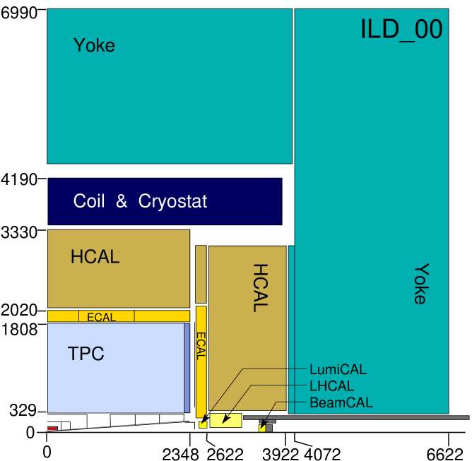
Figure 1: A quadrant of the “simulation baseline” configuration of the ILD detector. Distances are given in mm. From  [2].

The ILD detector is described in detail in [2]. For the present study the “simulation baseline” detector was used, which is shown in Fig. 1.

Of particular importance for the present studies are the main tracking detector (the TPC), the main electromagnetic calorimeter (the ECal), and the low angle calorimeters (the LumiCal, the LHCal and the BeamCal).

The track finding efficiency, even in high multiplicity events with overlaid beam background, is 99.5 % for momenta above 1 ${\mathrm{GeV}}$. The transverse momentum resolution ($\Delta(1/P_{T})=\Delta(P_{T})/P^{2}_{T}$) is expected to be $2.0\times 10^{-5}~{}\mbox{${\mathrm{GeV}}$}^{-1}$ asymptotically, worsening to $9.0\times 10^{-5}~{}\mbox{${\mathrm{GeV}}$}^{-1}$ at 10 ${\mathrm{GeV}}$, and to $9.0\times 10^{-4}~{}\mbox{${\mathrm{GeV}}$}^{-1}$ at 1 ${\mathrm{GeV}}$. In the low angle region, charged tracks will be efficiently detected down to $\theta=7^{\circ}$, while the only region not in the acceptance of the calorimetric system are the holes in the BeamCal for the beampipes. Around the outgoing beampipe, the radius of the hole is 20 mm at $z$=3550 mm, corresponding to 5.6 mrad. Since the crossing angle of the beams is 14 mrad and the hole for the incoming beampipe has R=16 mm, the lower edge of the acceptance increases to 18.5 mrad at $\phi\approx 180^{\circ}$. The ECal is a highly granular SiW sampling calorimeter with a transverse cell size of 5 mm $\times$ 5 mm and 20 layers. In test-beam measurements with a prototype detector a resolution of $(16.6\pm 0.1)/\sqrt{E(\mathrm{GeV})}\oplus(1.1\pm 0.1)\%$ has been achieved [2]. The simulation used here shows a similar resolution.

The ILD_00 detector model was fully simulated using the Geant4-based Mokka [11, 12] package. The model not only accounts for the active elements, but also for support structures, for cables and cooling systems, and dead regions in the sensitive layers. In the TPC, the properties of the P5 gas mixture was taken into account [13], resulting in a parametrisation of the point error depending on both drift distance and local track-pad angles. Two aspects of the detector, relevant for the present study, were simulated in less detail: The specific energy loss in the TPC was estimated by the theoretical Bethe-Bloch formula, taking into account the actual TPC geometry and read-out granularity, to yield an estimate of the separation power between different particle species [14]. This estimate was used to simulate the $dE/dx$-based particle identification on a track-by-track basis. Furthermore, the response of the BeamCal to high energy electrons was estimated by tracking the electron to the BeamCal, and then determining the probability of detection from a map of the expected energy density from beamstrahlung pairs, and a parametrisation of the probability to detect an electron of a given energy above a given background energy density. Both the map and the parametrisation were obtained from a separate full simulation study of the BeamCal alone.

The first means to increase the visibility of the $\tilde{\tau}$ signal above the background is to determine what beam parameters are the most favourable. Because SUSY itself poses a background problem in the $\tilde{\tau}$ analysis, it is required to run the ILC at the polarisation that minimises the background. For 100 % right e⁺ polarisation and 100 % left e^- polarisation ($\mathcal{P}_{beam}(e^{+},e^{-})$=(+1,$-$1)), the cross sections for $\tilde{\chi}^{0}_{2}$$\tilde{\chi}^{0}_{2}$ and $\tilde{\chi}^{+}_{1}$$\tilde{\chi}^{-}_{1}$ production are several 100 fb, and the branching ratios to $\tilde{\tau}$ are above 50 %. With the opposite polarisation, however, these cross sections will almost vanish. The SM cross sections are also reduced for $\mathcal{P}_{beam}$=($-$1,+1), albeit not so dramatically. In the case of the $\tilde{\tau}_{1}$, an added advantage is that the production cross section is enhanced by a factor of 3 for $\mathcal{P}_{beam}$=($-$1,+1) compared to the opposite case. For the $\tilde{\tau}_{2}$, the reverse is true, but the gain from the reduction of the background was found to be the more important feature. Hence, these channels were studied assuming $\mathcal{P}_{beam}$=($-$0.3,+0.8), the highest level of polarisation in the advantageous configuration attainable with the current baseline design of the ILC.

To generate events, the energy spectrum of the ILC beams were simulated first, including the effects of both the beamstrahlung and the energy spread from the main Linac. With these inputs, SUSY as well as Standard Model events were generated by Whizard [15]. All SM channels with up to 6 fermions in the final state were simulated. In addition, all 8 fermions final states passing the intermediate state $t\bar{t}f\bar{f}$ were also generated. For channels containing $\tau$ leptons, TAUOLA [16] was used to generate the $\tau$ decays. By default, the helicity of the $\tau$ is only internally generated in Whizard, so an interface between Whizard and TAUOLA was developed in order to correctly transfer this information between the two programs. In the case of $\gamma\gamma$ events, only multi-peripheral diagrams were included if the value of $Q^{2}$ was below 16 $\mbox{${\mathrm{GeV}}$}^{2}$. However, other types of diagrams (VDM, diffraction, etc.) do not produce events with large missing transverse momentum [4]. Except for the channel $\mbox{${\,e}^{+}{e}^{-}\to$}\gamma\gamma ee\rightarrow\tau\tau ee$, a further cut at generator level excluded all $\gamma\gamma$ events where the invariant mass of the $f\bar{f}$-pair was below $10~{}\mbox{${\mathrm{GeV}}$}$ from further treatment. It should be pointed out that the simulation also includes the $\gamma$-component of the incoming beams, so that the $\gamma\gamma$ sample also includes the processes when one or both of the $\gamma$’s are real.

In addition to these physics channels, the creation of $e^{+}e^{-}$ pairs due to the beamstrahlung process were generated, using GuineaPig [17], and simulated with Mokka. Some 125000 such low energetic pairs are expected to be created in each bunch crossing. A large fraction of these will leave the detector through the outgoing beampipe, but nevertheless the remaining pairs will deposit a large amount of energy in the BeamCal, and will create a large number of hits in the inner part of the tracking system. Approximately one additional charged particle per event will be detected in the TPC, and a large number of low energy photons will produce small showers in the calorimeters, or will convert in the tracking system. Due to the very large number of particles, this process cannot be simulated on an event-by-event basis, but rather a pool of 1000 bunch crossings was simulated separately. For each physics event, one such bunch crossing was selected at random, and overlaid to the event at the analysis stage.

The total simulated sample comprised some 13 million events. The samples generated for the 6 and 8 fermion channels corresponded to a integrated luminosity of at least 500 fb^-1. For the four fermion channels, the sample sizes for the channels not compatible with $\gamma\gamma$ (i.e. channels not having an $e^{+}e^{-}$-pair in the final state) corresponded to between 50 and 100 fb^-1, while the sample sizes of the channels compatible with $\gamma\gamma$ corresponded to 0.1 fb^-1 ($Q^{2}<16~{}\mbox{${\mathrm{GeV}}$}^{2}$ for both beam remnants), 1 fb^-1 ($Q^{2}<16~{}\mbox{${\mathrm{GeV}}$}^{2}$ for one beam remnant, $Q^{2}>16~{}\mbox{${\mathrm{GeV}}$}^{2}$ for the other), or 50 fb^-1 ($Q^{2}>16~{}\mbox{${\mathrm{GeV}}$}^{2}$ for both beam remnants). Finally, for the two fermion channels, the hadronic and muonic samples corresponded to 20 fb^-1, the $\tau^{+}\tau^{-}$ sample to 500 fb^-1, while the Bhabha channels corresponded to 1 fb^-1. (In the Bhabha sample, a generator level cut of $\cos{\theta}<0.96$ and $\cos{\theta_{acol}}<0.966$ was imposed). The total SM background expected at $E_{CMS}=500~{}\mbox{${\mathrm{GeV}}$}$ for an integrated luminosity of 500 fb^-1 was 4.92 $\times 10^{9}$ events, completely dominated by the $\gamma\gamma$ and Compton scattering processes. Apart from these two sources, the background was 1.53 $\times 10^{8}$ events, dominated by 9.94 $\times 10^{7}$ of $\mbox{${\,e}^{+}{e}^{-}\to$}\ell\ell$ events, mainly Bhabhas. The SUSY sample was divided into $\tilde{\tau}_{1}$$\tilde{\tau}_{1}$, $\tilde{\tau}_{2}$$\tilde{\tau}_{2}$ and other channels. In all categories, the generated sample corresponded to at least 500 fb^-1. The total number of expected events in the three categories were 7.92 $\times 10^{4}$, 8.85 $\times 10^{3}$, and 1.20 $\times 10^{4}$, respectively.

The simulated events were reconstructed with MarlinReco [18]. Tracks in the tracking system were reconstructed using the Kalman filter method, adopted from DELPHI [19], and the calorimetric signals were treated using the particle flow paradigm, implemented with Pandora  [20], with the PFOid package used for particle identification.

3 Mass, cross section and polarisation measurements

The key characteristics of $\tilde{\tau}$ production and decay, which single it out from the background, are:

• only two $\tau$ leptons in the final state

• large missing energy and momentum

• high acollinearity, with little correlation to the energy of the $\tau$ decay products

• central production

• no forward-backward asymmetry

Different backgrounds dominate for the $\tilde{\tau}_{1}$ and the $\tilde{\tau}_{2}$: for the $\tilde{\tau}_{1}$, the $\gamma\gamma$ background is important, while $WW\rightarrow l\nu l\nu$ is less important; the opposite is true for the $\tilde{\tau}_{2}$. For the mass measurement, the SUSY background is not very important, because it is dominated by $\tilde{\chi}^{\pm}_{1}$$\tilde{\chi}^{\mp}_{1}$ and $\tilde{\chi}^{0}_{2}$$\tilde{\chi}^{0}_{2}$ production with cascade decays over $\tilde{\tau}$ sleptons. In SPS1a’, the kinematic limits of these processes are well below those of both $\tilde{\tau}_{1}$ and $\tilde{\tau}_{2}$ pair production, so they have little influence on the determination of the endpoints of the spectra. For the polarisation measurement, the entire spectrum is needed, and hence the SUSY background becomes more important. Therefore the selection cuts differ for the single analyses, but nevertheless two sets of common initial cuts can be defined, one set to select the signal topology, and another to reject $\gamma\gamma$ events.

3.1 Topology selection

The first step in the topology selection was to group particles into jets. Jet finding was performed in two ways: for the polarisation analysis, where no beam induced background was overlaid, the standard Durham algorithm was used [21], forced to yield two jets. In the mass analysis, the overlaid beam induced background implies that such a method has too low an efficiency due to extra tracks and clusters from the background. In this case, reconstructed particles to be considered for the jet clustering were first selected by demanding that all particles should have an energy exceeding 500 ${\mathrm{MeV}}$, and that any charged particle should have at least one hit in the TPC. To exclude neutrals reconstructed from showers induced by the beam background, it was demanded that they should not be reconstructed from hits in the BeamCal, nor should the reconstructed starting-point of the shower be deep in the innermost part of the forward hadronic calorimeter ($|z|>3200$ mm and $r<500$ mm). Then the algorithm used in DELPHI to find $\tau$ leptons in $\tilde{\tau}$ events was used [22]. This algorithm - to be applied only after selecting low charged multiplicity events - goes through all possible combinations of charged tracks, trying to combine them into groups with invariant masses of $M_{jet}<2~{}\mbox{${\mathrm{GeV}}$}$, under the condition that if several such groupings were possible, the one with the lowest sum of jet-masses should be taken. In a second step, neutrals were added to the charged groups, still respecting the maximal mass. Any neutrals left over were labelled as belonging to the ROE group (“Rest Of Event”).

Events compatible with the $\tilde{\tau}$ topology were then selected in both analyses by requiring:

• exactly two jets

• less than 10 charged particle candidates

• vanishing total charge

• charge of each jet = $\pm 1$

• invariant jet masses $M_{jet}<2.5~{}\mbox{${\mathrm{GeV}}$}$ for both jets

• a total visible energy $E_{vis}<300~{}\mbox{${\mathrm{GeV}}$}$

• a missing mass $M_{miss}>250~{}\mbox{${\mathrm{GeV}}$}$

• no particle with momentum above $180~{}\mbox{${\mathrm{GeV}}$}$

Here $M_{miss}$, the invariant mass of the invisible system, is determined by the difference between the initial $e^{+}e^{-}$ system and the visible system. After these cuts, 9.23 $\times 10^{8}$ events remained in the standard model sample (2.41 $\times 10^{5}$ non-$\gamma\gamma$). In the three SUSY subsamples, 6.92 $\times 10^{4}$, 7.36 $\times 10^{3}$ and 8.41 $\times 10^{3}$ events remained at this stage.

3.2 Rejection of $\gamma\gamma$ events, and other SM processes

The characteristics of the $\gamma\gamma$ background is the presence of two highly energetic beam remnant electrons at low angles, while the rest of the event forms a system of low energy and mass. A veto against large energy deposits at small angles was therefore imposed. The events that remained did so because the beam remnants escaped the detector through the incoming or outgoing beampipe. This limits the missing transverse momentum $P_{T}$, and implies that the visible system consists of two fermions almost back-to-back in the transverse projection. In the direction of the incoming beampipe of the other beam, a much larger deflection of the beam remnant could pass undetected, so a cut on $P_{T}$ needs to depend on the azimuthal angle of the missing momentum.

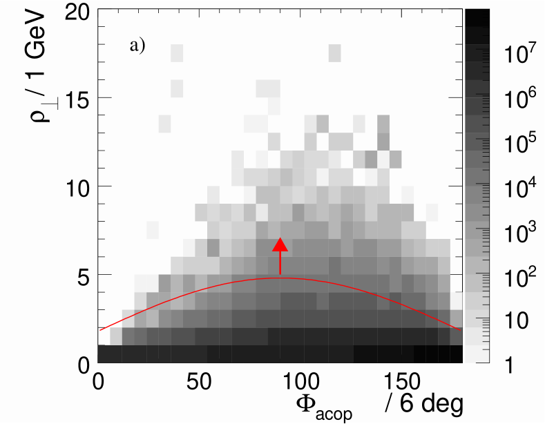
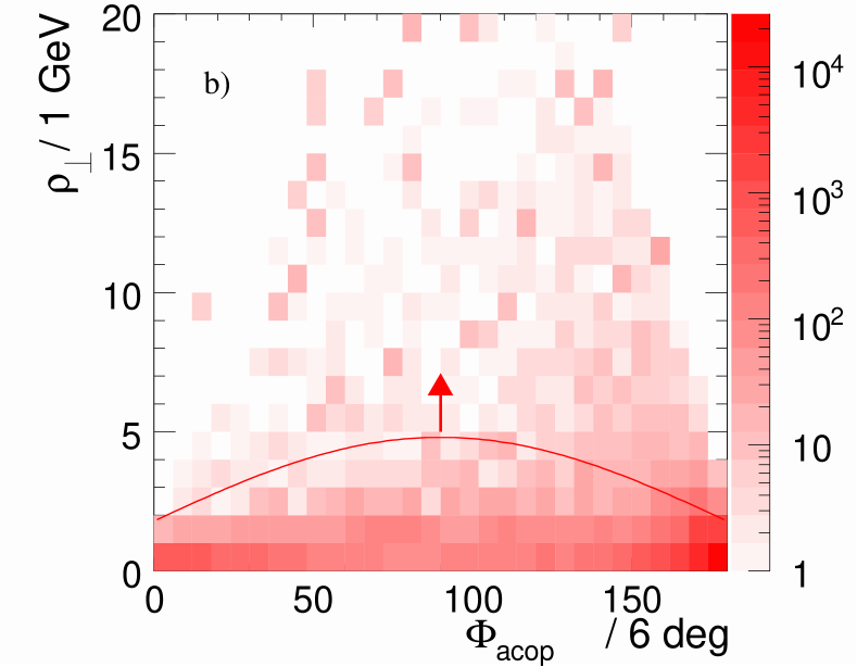
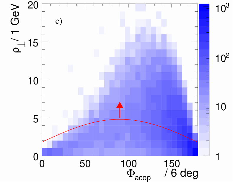
Figure 2: The distribution of the $\rho_{\perp}$ variable, defined in the text, versus the acoplanarity angle. a) $\gamma\gamma$ events, b) Other SM events, c) SUSY signal. The selected events are above the solid curve.

After the low angle veto, a $\gamma\gamma\rightarrow\tau\tau$ event could only have both high missing $P_{T}$ and large $\Phi_{acop}$ (the angle between the two jets projected to the plane perpendicular to the beam axis) if the decays of the two $\tau$ leptons were asymmetric: one of the $\tau$ leptons must have decayed with the visible products going close to opposite to the $\tau$ direction - giving a jet at large angle to the $\tau$, but low energy - while the other must have done the opposite - giving a jet with small angle to its parent $\tau$, and large energy. This property was exploited by the variable $\rho_{\perp}$,  the scalar sum of the transverse momenta of the jets w.r.t. the thrust axis, in the projection perpendicular to the beam [23]. Also $\mbox{${\,e}^{+}{e}^{-}\to$}\tau^{+}\tau^{-}$ events tend to have lower $\rho_{\perp}$ than the SUSY signal. Figure  2 shows the simultaneous distribution of $\rho_{\perp}$ and $\Phi_{acop}$ for signal and background events.

This lead to the following initial cuts to reduce the $\gamma\gamma$ background:

• $\rho_{\perp}>(2.7\sin{\Phi_{acop}}+1.8)~{}\mbox{${\mathrm{GeV}}$}$. A similar form of this cut was proposed in [24].

• no significant activity in the BeamCal

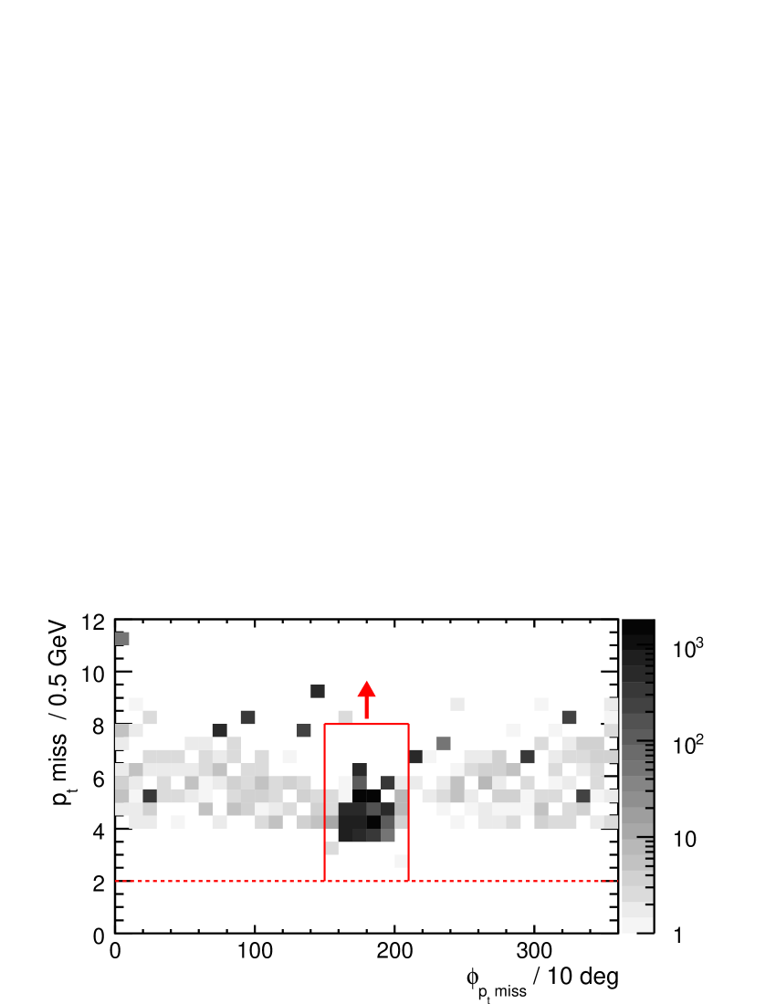
Figure 3: The distribution of the missing transverse momentum, $p_{{}_{t}miss}$, as a function of the azimuthal angle of the missing momentum, $\phi_{p_{t}miss}$. The accumulation of high $p_{{}_{t}miss}$ events around $\phi_{p_{t}miss}$= 180^∘ is clearly seen. It corresponds to $\gamma\gamma$ events with one beam remnant escaping in the incoming beampipe of the other beam. Events outside the (red) line were accepted.

• If the azimuthal angle of the missing momentum, $\phi_{p_{t}miss}$, was within 30^∘ to the direction of the incoming beampipe, the value of the missing transverse momentum should exceed $8~{}\mbox{${\mathrm{GeV}}$}$, see Fig. 3.

At this stage, 1.27 $\times 10^{6}$ events remained, of which 3.82 $\times 10^{4}$ were non-$\gamma\gamma$ events. The reduction of the $\tilde{\tau}_{1}$$\tilde{\tau}_{1}$ signal sample, as well as of the SUSY background sample, is sizable due to these cuts: 2.26 $\times 10^{4}$ events remained for $\tilde{\tau}_{1}$$\tilde{\tau}_{1}$, while 4.33 $\times 10^{3}$ remained for the background. The $\tilde{\tau}_{2}$$\tilde{\tau}_{2}$ sample, on the other hand, was little affected, due to its higher missing momentum: 6.26 $\times 10^{3}$ still remained.

In the single analyses, different cuts were used to further reduce this background to acceptable levels. They were intrinsically different for the various cases. The polarisation study relied on particle identification, and this also heavily constrained the background. In the $\tilde{\tau}_{2}$ analysis, the signal had high enough visible energy that the $\gamma\gamma$ background could easily be reduced.

In the study of the $\tilde{\tau}_{1}$ (both mass and polarisation in the $\pi$ channel), the following cuts were made in addition:

• $E_{vis}<120~{}\mbox{${\mathrm{GeV}}$}$,

• $|\cos{\theta_{jet}}|<0.9$ for both jets,

• $\Phi_{acop}>85^{\circ}$,

• $(E_{jet1}+E_{jet2})\sin{\Phi_{acop}}<30~{}\mbox{${\mathrm{GeV}}$}$.

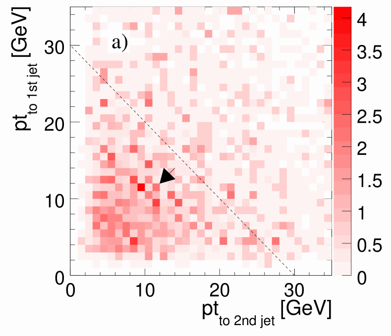
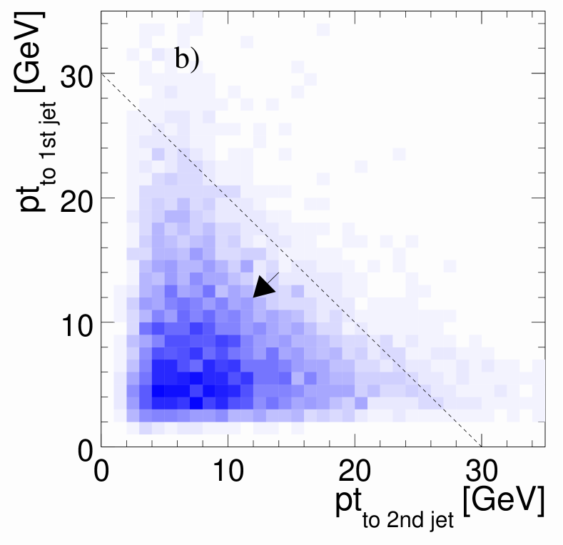
Figure 4: Transverse momentum of one jet w.r.t. the direction of the other jet. Left: SUSY background. Right: $\tilde{\tau}_{1}$ signal. The cut, given by the dashed line, corresponds to $(E_{jet1}+E_{jet2})\sin{\Phi_{acop}}<30$. The selected events are below the line.

The cut on $(E_{jet1}+E_{jet2})\sin{\Phi_{acop}}$, shown in Fig. 4, was effective because the remaining SUSY background came from decays of heavier sparticles, and thus tended to be less back-to-back than the signal. At this stage the SM background was reduced to 9.95 $\times 10^{4}$ events, of which 1189 were non-$\gamma\gamma$ events. 1.90 $\times 10^{4}$ $\tilde{\tau}_{1}$$\tilde{\tau}_{1}$ events remained, while the SUSY background was reduced to 2.51 $\times 10^{3}$ events.

3.3 $\tilde{\tau}$ endpoint and cross section

The $\tilde{\tau}$ mass can be extracted from the endpoint of the $E_{\tau}$ spectrum, which is equal to $E_{\tau,max}$, and the $\tilde{\chi}^{0}_{1}$ mass, known e.g. from a separate analysis of $\tilde{e}$ and $\tilde{\mu}$ decays. In principle, the maximum of the spectrum is at $E_{\tau,min}$, so that the $\tilde{\tau}$ channel can be used to determine $M_{\tilde{\chi}^{0}_{1}}$ as well, but due to the large $\gamma\gamma$ background, the turnover point is quite hard to observe.

In the analysis of both the $\tilde{\tau}_{1}$ and $\tilde{\tau}_{2}$ mass, two additional cuts were applied against the $\gamma\gamma$ background: The direction of the missing momentum vector was restricted to $|\cos{\theta_{miss}}|<0.8$. In events with more than 2 ${\mathrm{GeV}}$ of energy in the ROE group, at least 20 % of that energy should be observed at angles above $30^{\circ}$ to the beam axis. With these cuts, there were 2.22 $\times 10^{4}$ SM background events left in the sub-sample selected for the analysis of the $\tilde{\tau}_{1}$ properties (the “ $\tilde{\tau}_{1}$ sample” in the following). At this stage it is a subset of the sample selected for the analysis of the $\tilde{\tau}_{2}$  properties (the “$\tilde{\tau}_{2}$ sample”), which still contains 1.15 $\times 10^{5}$ SM events. The remaining signal in the two cases was 1.40 $\times 10^{4}$ for $\tilde{\tau}_{1}$$\tilde{\tau}_{1}$, and 4242 for $\tilde{\tau}_{2}$$\tilde{\tau}_{2}$. In addition, the $\tilde{\tau}_{1}$ sample contained 214 $\tilde{\tau}_{2}$$\tilde{\tau}_{2}$ events, and 1559 other SUSY events, while the $\tilde{\tau}_{2}$ sample contained 1.56 $\times 10^{4}$ $\tilde{\tau}_{1}$$\tilde{\tau}_{1}$ events, and 3033 other SUSY events.

3.3.1 $\tilde{\tau}_{1}$ endpoint and cross section

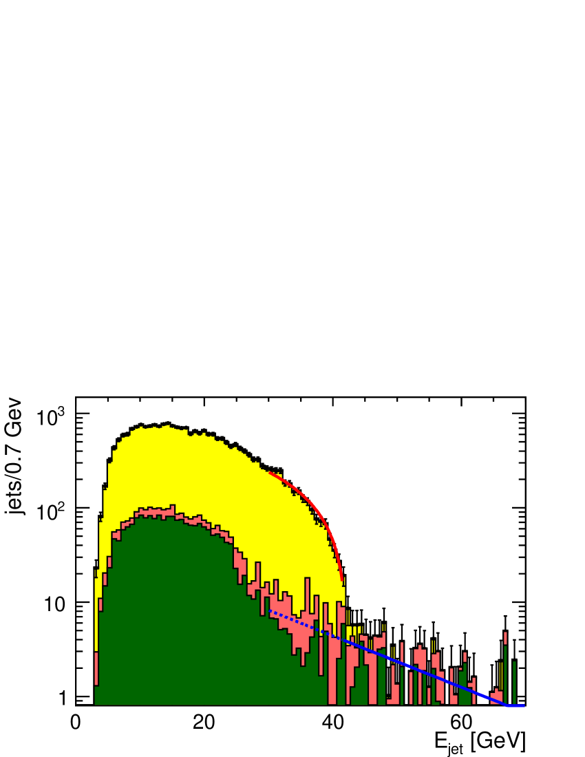
Figure 5: The jet energy spectrum of events selected in the $\tilde{\tau}_{1}$ endpoint analysis, with one entry per jet. Light grey (yellow) histogram: signal, grey (red) : SM background, dark grey (green): SUSY background. The fit to the background in blue. It is fitted in the signal-free region to the right (solid portion of the line), and extrapolated into the signal region (dashed). Fit to total sample: Solid (red) line. The endpoint is at the cross-over of the two lines.

For the $\tilde{\tau}_{1}$ sample, it was finally demanded that the mass of the visible system, $M_{vis}$, be above 20 ${\mathrm{GeV}}$ and below 87 ${\mathrm{GeV}}$. After these cuts, 10244 $\tilde{\tau}_{1}$ signal events remained (14.85 % efficiency), while the SM background amounts to 323.5 events. The total SUSY background contained 1029.6 events, including a contribution of 170.0 $\tilde{\tau}_{2}$ events. Fig. 5 shows that the endpoint was almost background free. The turnover point, which is equal to the minimal $\tau$ energy $E_{\tau,min}=2.6~{}\mbox{${\mathrm{GeV}}$}$ for most decay channels, was too distorted by the cuts to be measurable.

The remaining background close to the endpoint - in the range between 30 and 70 ${\mathrm{GeV}}$ - was found to be well described by an exponential, and was fitted in the signal-free region above 44 ${\mathrm{GeV}}$. The background fit was subtracted from the observed spectrum, and the background-subtracted spectrum was fitted with a straight line in the range from 30 to 41.5 ${\mathrm{GeV}}$. As the dominating background stems from SM processes, it can be argued that, once ILC data is available to tune the SM simulation, the background will be known to a precision much better than what can be determined from the present simulation. Therefore, the error on the expectation value of the background was assumed to be negligible compared to its Poisson fluctuations. Hence, the error on the background fit was not propagated into the statistical errors. Under these assumptions, the result of the fit was $E_{\tau,max}=42.11^{+0.14}_{-0.12}~{}\mbox{${\mathrm{GeV}}$}$. One notes that this number is not compatible with the true value ($42.54~{}\mbox{${\mathrm{GeV}}$}$, with mass effects in the $\tau$ decay included). The difference is 1.1%, equal to 3.1 $\sigma$. It reflects the fact that a straight line is not quite adequate to describe the spectrum near the endpoint. For a final analysis a more sophisticated function would be needed, either theoretical (including the properties of the different decay channels and their branching ratios), or by building MC generated templates.

Fitting $M_{\tilde{\tau}_{1}}$ instead of the endpoint position, the result was $\mbox{$M_{\tilde{\tau}_{1}}$}=107.73^{+0.03}_{-0.05}$ ${\mathrm{GeV}}$. (The true value in SPS1a’ is $\mbox{$M_{\tilde{\tau}_{1}}$}=107.86~{}\mbox{${\mathrm{GeV}}$}$.) However, this result assumes that $M_{\tilde{\chi}^{0}_{1}}$ is known. At this model point, the derivative of $M_{\tilde{\tau}_{1}}$ w.r.t. $M_{\tilde{\chi}^{0}_{1}}$ is 1.1, so the actual error on $M_{\tilde{\tau}_{1}}$ is 30 ${\mathrm{MeV}}$ $\oplus$ 1.1$\cdot\delta\mbox{$M_{\tilde{\chi}^{0}_{1}}$}$. In [25], an analysis of $\tilde{\mu}_{\mathrm{L}}$$\tilde{\mu}_{\mathrm{L}}$ production using the same fully simulated sample was presented. The author found $\delta{\mbox{$M_{\tilde{\chi}^{0}_{1}}$}}=1100~{}\mbox{${\mathrm{MeV}}$}$ from this channel alone, so using all $\tilde{\mu}$ and $\tilde{e}$ channels, one could expect that $\delta{\mbox{$M_{\tilde{\chi}^{0}_{1}}$}}\approx 250~{}\mbox{${\mathrm{MeV}}$}$. This is still a very conservative number, since previous fast simulation studies of $\tilde{\mu}_{\mathrm{R}}$$\tilde{\mu}_{\mathrm{R}}$ and $\tilde{e}_{\mathrm{R}}$$\tilde{e}_{\mathrm{R}}$ production in similar, though not identical scenarios found $\delta\mbox{$M_{\tilde{\chi}^{0}_{1}}$}\approx 200~{}\mbox{${\mathrm{MeV}}$}$ and $\delta{\mbox{$M_{\tilde{\chi}^{0}_{1}}$}}\approx 80~{}\mbox{${\mathrm{MeV}}$}$, respectively [24]. In the most optimistic case, the relative error $\Delta(\mbox{$M_{\tilde{\tau}_{1}}$})/\mbox{$M_{\tilde{\tau}_{1}}$}$ is 0.09 %, a value still dominated by $\delta{\mbox{$M_{\tilde{\chi}^{0}_{1}}$}}$.

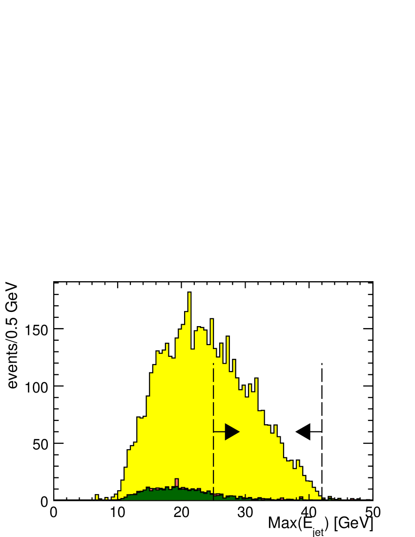
Figure 6: The spectrum of the highest jet energy of events selected in the $\tilde{\tau}_{1}$ cross section analysis, with one entry per event. Light grey (yellow) histogram: signal, grey (red): SM background, dark grey (green): SUSY background. The cross section was estimated by the number of events having max($E_{jet}$) between 25 and 42 ${\mathrm{GeV}}$, as indicated by the vertical lines.

The “effective” cross section, i.e. the cross section for the beam energy spectrum and the polarisation actually delivered by the ILC, was measured as follows: As the main background in this analysis arose from other SUSY channels, one could not assume that the background was known with arbitrarily good precision from simulation, as one can argue for the SM background. It needed either to be estimated from data, or to be reduced so much that even a very large uncertainty of its expected level had little influence on the final number. In principle, one could use the fact that the $\tilde{\tau}_{1}$ signal is decreased in $\mathcal{P}_{beam}=(+0.3,-0.8)$, while the SUSY background is largely enhanced to get an equivalent, but almost signal-free, sample. However, it was quite difficult to reduce the $\tilde{\tau}_{1}$ signal to negligible levels. This would necessitate a thorough study of the $\tilde{\chi}^{\pm}_{1}$ channel, which was beyond the scope of the present study. Instead, another approach was used: by requiring that at least one jet had an energy above 25 ${\mathrm{GeV}}$, and none had an energy above 42 ${\mathrm{GeV}}$, and that no jet was identified as a single lepton, the total SUSY background was reduced to 49 events, accompanied by 18 SM events, while 2226 signal events still remained. The $\max(E_{jet})$ spectrum in this sample is shown in Fig. 6.

Assuming that the uncertainty on the SUSY background is 100 %, this yielded a relative uncertainty on the expected number of signal events $\Delta(N_{signal})/N_{signal}=3.1~{}\%$

This number of events gave an “effective” cross section $\sigma_{eff}$=$N_{signal}/(\mathcal{L}\epsilon_{signal})$=$158.4\pm 4.9$ fb. The value is, by construction, equal to the expected one, and the error only comes from the uncertainty on $N_{signal}$: The uncertainty on $\mathcal{L}$ is expected to be $<$ 0.1 %  [26], i.e. negligible w.r.t. 3.1 %. For the present analysis, the error on $\epsilon_{signal}$ is 2 %, but this number could be made significantly smaller with a larger simulated sample.

In the cross section, $M_{\tilde{\tau}_{1}}$ only enters via an overall factor $\beta^{3}$ : $\sigma_{\mbox{$\tilde{\tau}_{1}$}}=A\times\beta^{3}/s$, where $A$ is a function of $\theta_{\mbox{$\tilde{\tau}$}}$ and $\mathcal{P}_{beam}$. This gives $\mbox{$M_{\tilde{\tau}_{1}}$}=E_{beam}\sqrt{1-(\sigma s/A)^{2/3}}$, and the error on the mass is

$$\Delta^{2}(\mbox{$M_{\tilde{\tau}_{1}}$})= (\frac{d\mbox{$M_{\tilde{\tau}_{1}}$}}{d\sigma})^{2}\Delta(\sigma)^{2}+(\frac{d\mbox{$M_{\tilde{\tau}_{1}}$}}{dE})^{2}\Delta(E)^{2}+$$

$$(\frac{d\mbox{$M_{\tilde{\tau}_{1}}$}}{dA})^{2}\Delta(A)^{2}$$

Considering this at fixed $A$,

$$\frac{\Delta(\mbox{$M_{\tilde{\tau}_{1}}$})}{\mbox{$M_{\tilde{\tau}_{1}}$}}=\frac{\sqrt{(\frac{\Delta(\sigma)}{\sigma}\beta^{2})^{2}+(\frac{\Delta(E)}{E}(3-5\beta^{2}))^{2}}}{3(1-\beta^{2})}$$

The design goal for the ILC is $\frac{\Delta(E)}{E}\leq 0.1$% [27], so for SPS1a’, and the given $E_{beam}$, the second term is negligible, and $\Delta(\mbox{$M_{\tilde{\tau}_{1}}$})/\mbox{$M_{\tilde{\tau}_{1}}$}=(\Delta(\sigma)/\sigma)(\beta^{2})/3(1-\beta^{2})$= 2.1 %.

Finally, it can be noted that, assuming the background and signal selection efficiencies remain the same, the optimal centre-of-mass energy for determining $M_{\tilde{\tau}_{1}}$ from the cross-section is 250 ${\mathrm{GeV}}$. With these assumptions, the error on the mass is reduced to a quarter, i.e. $\Delta(\mbox{$M_{\tilde{\tau}_{1}}$})/\mbox{$M_{\tilde{\tau}_{1}}$}$ = 0.5 %. It is most probable that the background levels would be substantially lower, since there is no SUSY background at $E_{CMS}$ = 250 ${\mathrm{GeV}}$. It is possible that the SM background would increase, due to the change of cuts needed to accommodate the change in signal characteristics: $E_{\tau,min}$ increases to 5.7 ${\mathrm{GeV}}$, while $E_{\tau,max}$ decreases to 16.9 ${\mathrm{GeV}}$. However, this would only mean trading a poorly known SUSY background for a well known SM one.

3.3.2 $\tilde{\tau}_{2}$ endpoint and cross section

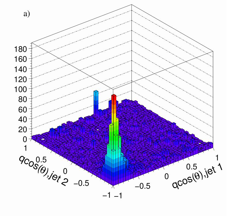
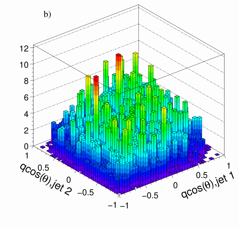
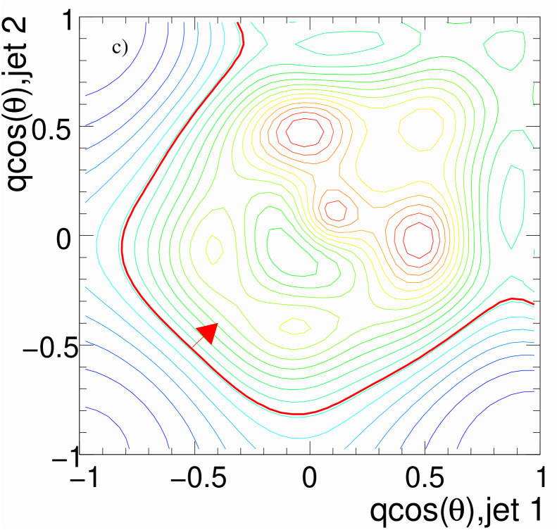
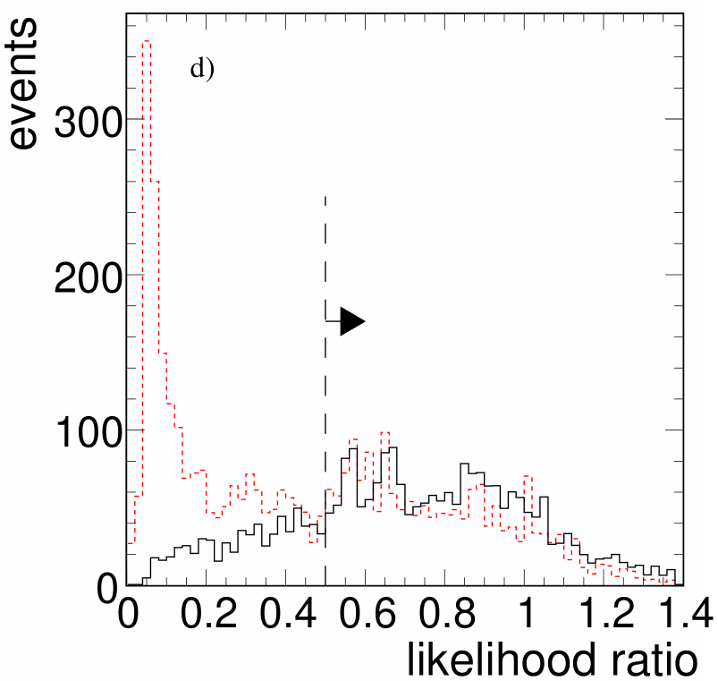
Figure 7: Upper two figures: lego plots of $q_{jet}\cos{\theta_{jet}}$ for the two jets. a): $WW$ events, b): signal. Lower two figures: c) multi-quadratic fit to the ratio between signal and background. The thicker line indicates the cut: events inside this contour were accepted, as indicated by the arrow. d): Distribution of the likelihood ratio for signal (solid black) and background (dashed red). The vertical line indicates the cut.

For the $\tilde{\tau}_{2}$ sample, it was demanded that $E_{vis}>50~{}\mbox{${\mathrm{GeV}}$}$, and $\Phi_{acop}<155^{\circ}$, and the energy of the ROE-group was below 10  ${\mathrm{GeV}}$. These cuts left 8095 SM background events, 3500 of which were from $WW\rightarrow l\nu l\nu$, the rest being $ZZ\rightarrow ll\nu\nu$ or six-fermion events. In the $\tilde{\tau}_{2}$$\tilde{\tau}_{2}$ sample, 3156 events remained, while 360 SUSY background and 339 $\tilde{\tau}_{1}$$\tilde{\tau}_{1}$ events also passed the cuts. As the main background at this level was found to be $WW\rightarrow l\nu l\nu$, it was requested that the other jet was not a single electron or muon, since the probability, in $WW\rightarrow l\nu l\nu$ events, that a genuine $\tau$ from one $W$-decay is accompanied by an electron or muon on the other side is 78 %, while it is only 35 % for a $\tau$ from a $\tilde{\tau}$ decay. At this point, most SUSY background events had a maximum kinematically allowed jet energy well below the endpoint of the $\tilde{\tau}_{2}$ spectrum. Only $\tilde{\mu}_{\mathrm{L}}$$\tilde{\mu}_{\mathrm{L}}$ and $\tilde{e}_{\mathrm{L}}$$\tilde{e}_{\mathrm{L}}$ events where one of the sleptons decayed in a cascade via a $\tilde{\chi}^{\pm}_{1}$ to a $\tau$ remained. These events were rejected by requiring that the most energetic jet should not be an electron or a muon. Finally, a likelihood ratio was formed of the joint distributions of $q_{jet1}\cos{\theta_{jet1}}$ and $q_{jet2}\cos{\theta_{jet2}}$ for signal and SM background, as shown in Fig. 7. The jet charges $q_{jet,i}$ are determined by the charge sum of the tracks in the jet, without any momentum weighting. The ratio of the two distributions was symmetrised along the diagonal and fitted with a multi-quadratic function, in order to smooth out the statistical fluctuations. The likelihood ratio exploits the fact that the distribution of lepton momenta in $WW\rightarrow l\nu l\nu$ events is forward peaked and forward-backward asymmetric, contrary to the signal. The final SM background was 2257 jets in 1533 events, while the signal was 3227 jets in 1972 events (22.3 % efficiency). In addition 418 (4) jets in 233 (3) events survived in the $\tilde{\tau}_{1}$$\tilde{\tau}_{1}$ (SUSY background) sample.

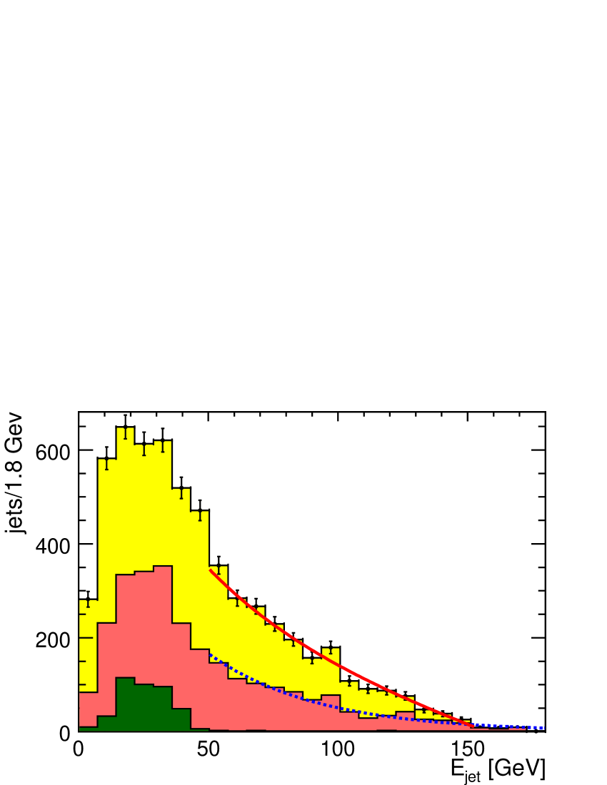
Figure 8: The jet energy spectrum of events selected in the $\tilde{\tau}_{2}$ endpoint analysis, with one entry per jet. Light grey (yellow) histogram: signal, grey (red): SM background, dark grey (green): SUSY background. The fit to the background is indicated by the dashed (blue) line. It was fitted to the background only simulation. Fit to total sample: solid (red) line. The endpoint is at the cross-over of the two lines.

The endpoint of the spectrum was determined by first estimating the background. As virtually no SUSY background was present at the endpoint, it was assumed that the expected background level was known to a much better precision than its Poisson fluctuations. The simulated background was parametrised by an exponential function, and the signal was fitted by a straight line added to the exponential. The spectrum and the fitted functions are shown in Fig. 8. It should also be pointed out that only the decay mode $\mbox{$\tilde{\tau}_{2}$}\rightarrow\tau\mbox{$\tilde{\chi}^{0}_{1}$}$ contributes in the region where the fit was done: the cascade decays via a $\tilde{\chi}^{\pm}_{1}$ yield jets of energies of at most 25 ${\mathrm{GeV}}$.

The endpoint was found to be $E_{\tau,max}=150.2^{+2.0}_{-1.7}~{}\mbox{${\mathrm{GeV}}$}$. In this case, the simple straight line fit is sufficient: the value found is compatible with the true value ($152.2~{}\mbox{${\mathrm{GeV}}$}$). Fitting the mass gave $\mbox{$M_{\tilde{\tau}_{2}}$}=183^{+11}_{-5}~{}\mbox{${\mathrm{GeV}}$}$, assuming the true value for $M_{\tilde{\chi}^{0}_{1}}$. At this point, $M_{\tilde{\tau}_{2}}$ is very sensitive to $M_{\tilde{\chi}^{0}_{1}}$: $d\mbox{$M_{\tilde{\tau}_{2}}$}/d\mbox{$M_{\tilde{\chi}^{0}_{1}}$}$ = 18, so an error of 80 ${\mathrm{MeV}}$ on $M_{\tilde{\chi}^{0}_{1}}$ translates into an additional error of 1.4 ${\mathrm{GeV}}$ on $M_{\tilde{\tau}_{2}}$. The relative error $\Delta(\mbox{$M_{\tilde{\tau}_{2}}$})/\mbox{$M_{\tilde{\tau}_{2}}$}$ is 3.6 %, which is dominated by the error on the end-point measurement.

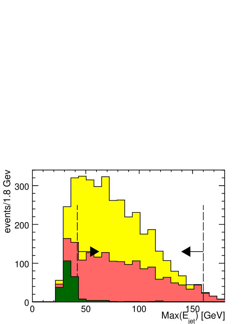
Figure 9: The spectrum of the maximum jet energy of events selected in the $\tilde{\tau}_{2}$ cross section analysis, with one entry per event. Light grey (yellow) histogram: signal, grey (red): SM background, dark grey (green): SUSY background. The cross section was estimated by the number of events having max($E_{jet}$) between 42 and 160 ${\mathrm{GeV}}$, as indicated by the vertical lines.

To determine the “effective” cross section, a sample of events was extracted consisting of those where any of the two jets were accepted for the endpoint measurement. The events which had no jet with energy above the endpoint in $\tilde{\tau}_{1}$ production (42 ${\mathrm{GeV}}$) or with one jet well beyond the endpoint of $\tilde{\tau}_{2}$ production (160 ${\mathrm{GeV}}$) were excluded. With these additional conditions, the sample contained 1765 $\tilde{\tau}_{2}$ events, 1374 SM ones, and only 33 other SUSY events. The distribution of events is shown in Fig. 9. This yielded $\Delta(N_{signal})/N_{signal}=4.2~{}\%$, assuming again a 100% uncertainty on the SUSY background, and a negligible uncertainty on the SM background.

The corresponding “effective” cross section was $\sigma_{eff}$= $N_{signal}/(\mathcal{L}\epsilon_{signal})$= $17.7\pm 0.7$ fb, where once again the uncertainty on $\mathcal{L}$ and $\epsilon_{signal}$ are assumed to be negligible compared to $\Delta(N_{signal})$.

Also for the $\tilde{\tau}_{2}$, the relative error on the beam energy is small compared to that of the error on the cross section, so that $\Delta(\mbox{$M_{\tilde{\tau}_{2}}$})/\mbox{$M_{\tilde{\tau}_{2}}$}$ = $(\Delta(\sigma)/\sigma)(\beta^{2})/3(1-\beta^{2})$ = 2.4 %. The relative error on the mass obtained from the cross section is thus as small for $\tilde{\tau}_{2}$ as for $\tilde{\tau}_{1}$ although the cross section is more than 10 times smaller and the background is much larger. This is due to the fact that there is almost no (poorly known) SUSY background in the former, and that it is on the rising edge of the cross section vs. $\sqrt{s}$ curve at $\sqrt{s}$ = 500 ${\mathrm{GeV}}$.

If, finally, the values of the endpoint and $M_{\tilde{\tau}_{2}}$ were used to calculate $M_{\tilde{\chi}^{0}_{1}}$, one finds an error of 1.7 ${\mathrm{GeV}}$, not including the error on $\theta_{mix}$.

3.4 $\tau$ polarisation

In this analysis, the $\tau\rightarrow\pi^{\pm}\nu_{\tau}$ and $\tau\rightarrow\rho^{\pm}\nu_{\tau}\rightarrow\pi^{\pm}\pi^{0}\nu_{\tau}$ modes have been studied [29]. These modes have already been the subject of fast simulation analyses, e.g. in [3] and [10].

As explained in the introduction, the compositions of the $\tilde{\tau}$ and the $\tilde{\chi}^{0}_{1}$ manifest themselves in the probability that the $\tau$ has either helicity, i.e. in the $\tau$ polarisation, $\mathcal{P}_{\tau}$. To observe $\mathcal{P}_{\tau}$, one uses the fact that only one helicity state exists for $\nu_{\tau}$, which induces a angular distribution $\propto 1-a\mathcal{P}_{\tau}\cos{\psi}$ for the visible decay products in the $\tau$ rest frame [28] ($\psi$ is the angle between the helicity axis and the momentum, and $a$ is a factor depending on the mass and spin of the $\tau$ decay product). The lab frame energy spectrum is therefore sensitive to $\mathcal{P}_{\tau}$. If, in addition, the decay product is a vector, the probability of the product being transversely or longitudinally polarised also depends on $\mathcal{P}_{\tau}$: one case would correspond to a (more likely) conservation of helicity, the other to a (less likely) helicity flip. Whether the vector particle is transverse or longitudinal can be determined by the angular distribution of its decay products: in the rest frame of a two-body decay to scalars, the products tend to line up along the spin axis in the longitudinal case ($\xi=0$), and to be perpendicular to it in the transversal case ($\xi=\pi/2$). In the lab frame, the longitudinal case therefore corresponds to a case where the energies of the two scalars are maximally different, while in the transversal case they tend to be quite similar. In particular, the variable $R=E_{1}/(E_{1}+E_{2})$ is distributed as $(1-\beta_{vector}\cos(\xi))$, which is quite insensitive to the lab frame energy of the vector particle, once it is substantially larger than its mass (i.e. $\beta\approx 1$). $R$ will be distributed as $(R-1/2)^{2}$ for the longitudinal case, and as $1/4-(R-1/2)^{2}$ in the transversal case [3] [28]. In SPS1a’, the mixing is not particularly large, and $\tilde{\tau}_{1}$ is expected to be mainly right-handed. Hence, $\mathcal{P}_{\tau}$ is expected to be rather close to +1, and the spectrum in the $\tau\rightarrow~{}scalar$ should be harder than for the other helicity. In the case $\tau\rightarrow~{}vector$, the vector meson is mainly longitudinal, yielding an $R$ distribution peaking close to 0 and 1.

3.4.1 The $\tau\rightarrow\pi^{\pm}\nu_{\tau}$ channel

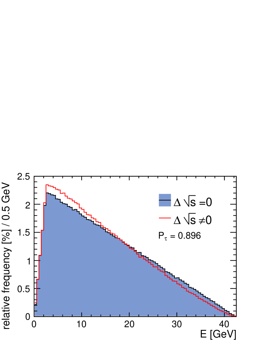
Figure 10: The simulated energy spectrum the pions in $\mbox{$\tilde{\tau}_{1}$}\rightarrow\tau\rightarrow\pi^{\pm}\nu_{\tau}$. The filled histogram shows the distribution for $E_{CMS}\equiv$ 500 ${\mathrm{GeV}}$ and ISR switched off in the generator, while the open one shows the spectrum with the ILC beam spectrum and ISR included.

The spectrum of the pions in the decay chain $\mbox{$\tilde{\tau}$}\rightarrow\tau\mbox{$\tilde{\chi}^{0}_{1}$}\rightarrow\pi^{\pm}\nu_{\tau}\mbox{$\tilde{\chi}^{0}_{1}$}$ is shown in Fig. 10, with and without ISR and beam energy spread. As the effect of these two factors clearly are not negligible, the true spectra were determined for extreme polarisations ($+1$ or $-1$), and parametrised correction functions were calculated for both cases. These functions were double polynomials of degree 2, the two pieces being applied above or below $E_{\tau,min}$, respectively. With these parametrisations ($F(E,+1)$ and $F(E,-1)$) at hand, the true spectrum for any polarisation can be obtained by applying the combined correction

$$F(E,\mathcal{P}_{\tau})=\frac{1+\mathcal{P}_{\tau}}{2}F(E,+1)+\frac{1-\mathcal{P}_{\tau}}{2}F(E,-1)$$

It should be noted that the highest sensitivity to the polarisation is in the region with $E_{\pi}<E_{\tau,min}$.

To extract the signal, the cuts described in Sects. 3.1 and 3.2 were supplemented by demanding that $E_{vis}$ be less than $90~{}\mbox{${\mathrm{GeV}}$}$, and that none of the jets had an energy exceeding $60~{}\mbox{${\mathrm{GeV}}$}$. The events should contain at least one signal decay candidate, defined as a jet that only contained a single particle, and that that particle was charged. After these cuts, there were 8.41$\times 10^{4}$ SM events (839 non $\gamma\gamma$), 201 $\tilde{\tau}_{2}$$\tilde{\tau}_{2}$ events, and 1678 other SUSY events remaining. 10730 $\tilde{\tau}_{1}$$\tilde{\tau}_{1}$ events remained, i.e. 21460 $\tilde{\tau}_{1}$ decays. In 4047 of these, the subsequent $\tau$-decay was the signal-channel $\tau\rightarrow\pi\nu_{\tau}$.

To reject $\tau\rightarrow\ell\nu_{\tau}\nu_{\ell}$ and $\tau\rightarrow K\nu_{\tau}$ from the sample of signal candidate jets, the full power of particle identification of the ILD was employed: The result from the PFOid package, which is based on the calorimetric measurements, was supplemented by the measurement of $dE/dx$ in the TPC. Only about 0.4 % of the non-signal decays were misidentified, while the efficiency to accept signal decays was 80 %.

This requirement was also very efficient in rejecting the remaining $\gamma\gamma$ background, since only a small fraction of these events did contain two $\tau$ leptons. The same was true for 4- and 6-fermion background, albeit to a lesser extent. The background from non-$\tilde{\tau}_{1}$$\tilde{\tau}_{1}$ SUSY channels, on the other hand, largely contained two $\tau$ leptons and was reduced only sightly more than the signal. It was nevertheless concluded that no further cuts were needed, and the final selection contained 3311 signal jets, 126 other decay modes of $\tilde{\tau}_{1}$, 334 other SUSY decays, and 122 SM jets.

The procedure to extract the polarisation in the presence of background was to first fit a heuristic function to the simulated background alone. The signal selection cuts were then applied to the signal+background sample, and the function describing the background was subtracted from the observed distribution. An efficiency correction function, determined from signal-only simulation, was applied. As the efficiency could possibly be dependent on the helicities of the two $\tau$ leptons in the event, the efficiency correction was parametrised as

$$\epsilon(E,\mathcal{P}_{\tau})= \left(\frac{1-\mathcal{P}_{\tau}}{2}\right)^{2}\epsilon_{--}(E)+\left(\frac{1-\mathcal{P}^{2}_{\tau}}{2}\right)\epsilon_{+-}(E)+$$

$$\left(\frac{1+\mathcal{P}_{\tau}}{2}\right)^{2}\epsilon_{++}(E)$$

The efficiencies $\epsilon_{--}(E),\epsilon_{+-}(E)$, and $\epsilon_{++}(E)$, correspond to the cases of the $\tau$ leptons being both of negative, of opposite, or both of positive helicity, respectively. These functions were separately determined from dedicated fast simulation samples with the corresponding helicity configurations.

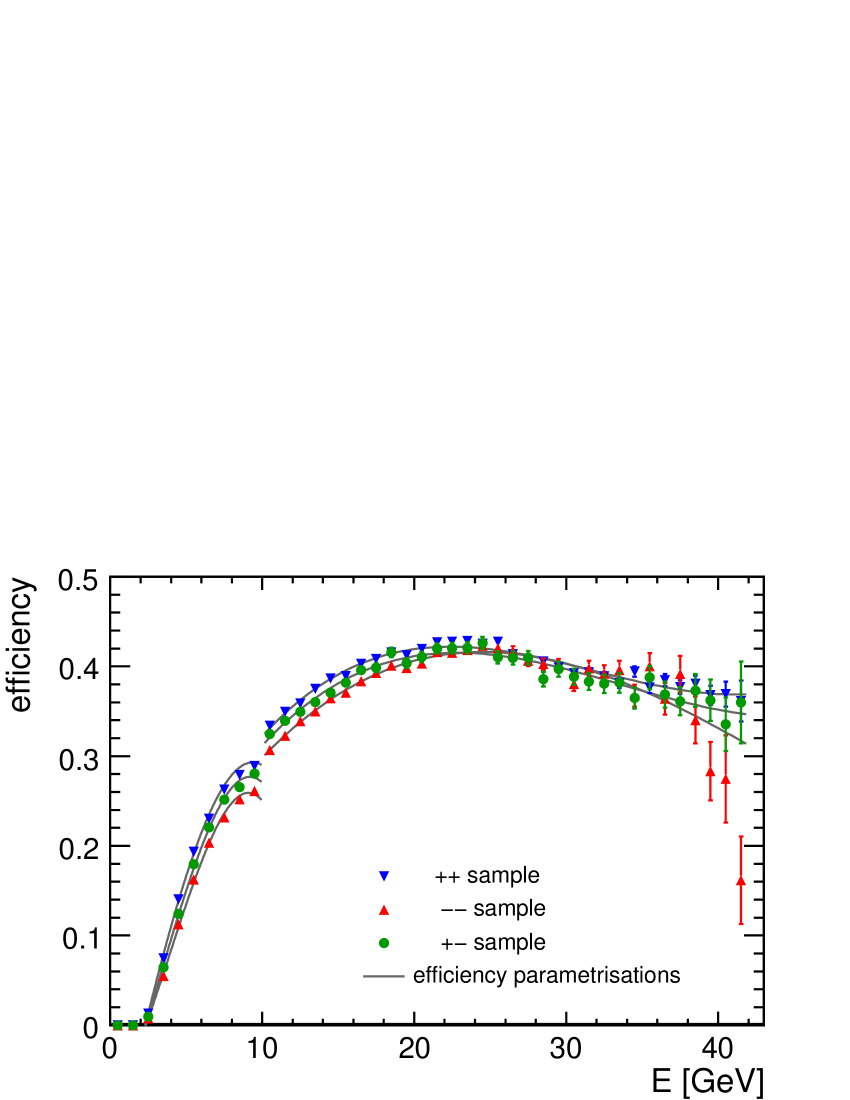
Figure 11: Ratio of the spectra before and after selection (points), and fitted efficiencies (lines) for different combinations of $\tau$ helicity. Inverted triangles (blue): both $\tau$ leptons are right-handed. Circles (green): the $\tau$ leptons have opposite helicity. Triangles (red): both $\tau$ leptons are left-handed. The discontinuity at 10 ${\mathrm{GeV}}$ is due to the fact that the particle identification algorithm changes from one set of p.d.f.s to another at that energy.

The ratios between initial and selected spectra are shown in Fig. 11, together with the fitted efficiency functions. A slight dependence on $\mathcal{P}_{\tau}$ was indeed observed and was found to be primarily caused by the cut on $\rho_{\perp}$.

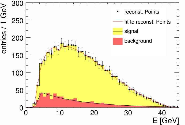
Figure 12: The energy spectrum of the selected pions. Light grey (yellow) histogram: signal. Dark grey (red) histogram: background. Black line: background fit. Grey (red) line: overall fit. The “dent” in the overall fit at $E_{\pi}$=10 ${\mathrm{GeV}}$ is due to the discontinuity of the efficiency parametrisation, see Fig. 11.

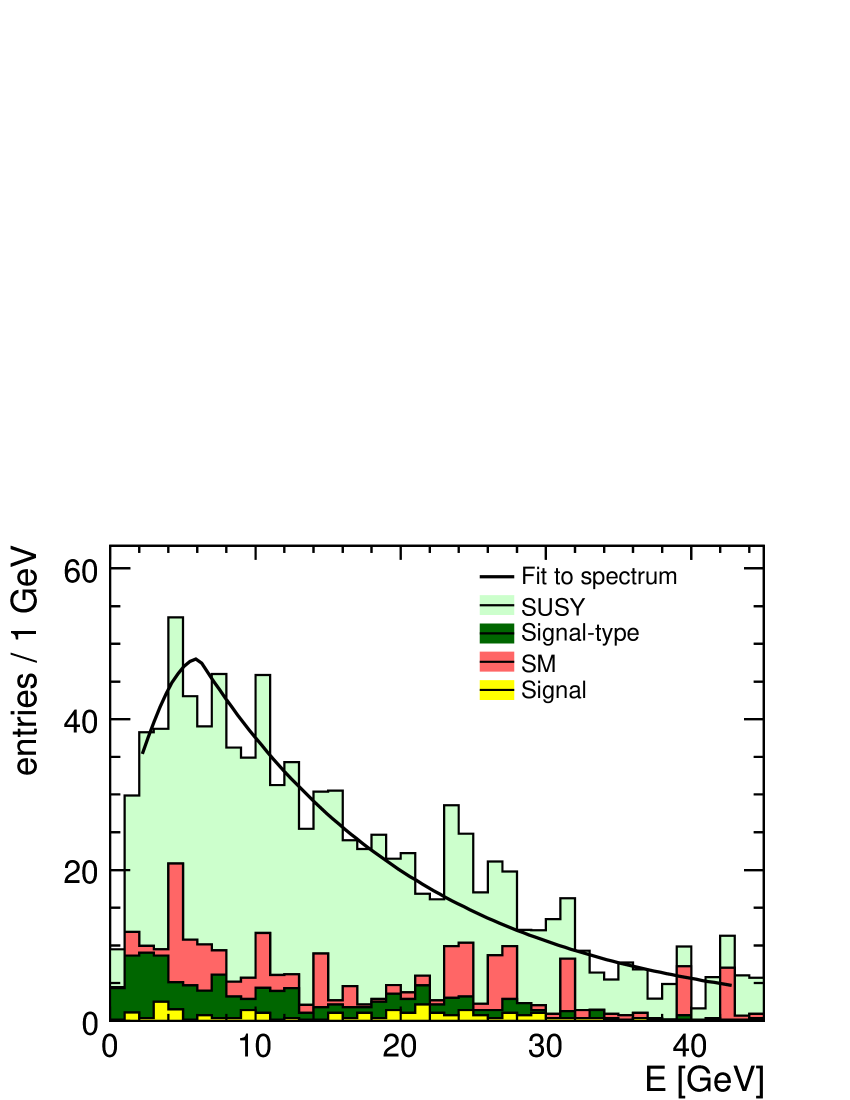
Figure 13: Energy spectrum of the pion candidates in the control sample. Light grey (light green) histogram: SUSY background (non-$\tilde{\tau}_{1}$). Grey (red) histogram: SM. Dark grey (dark green) histogram: SUSY background from other decays of the $\tau$ from $\tilde{\tau}_{1}$. Medium light grey (yellow) histogram: signal. Line: fit to spectrum.

The resulting distribution was then fitted with the theoretical spectrum, corrected for ISR and beam spread, and the polarisation was obtained, see Fig. 12. Assuming an integrated luminosity of 500 fb^-1, the value found was $\mathcal{P}_{\tau}=(91\pm 10)$ %, where the error is statistical. The expected value in SPS1a’ is 89.6 %. The fitted normalisation and the polarisation showed a quite sizable correlation, so if the normalisation was calculated using the value and uncertainty of the “effective” cross section obtained in section  3.3.1, the error on the polarisation decreased to 6 %. The uncertainty of the average background stemmed from the uncertainty on its SUSY component, while the average of the SM component would have a negligible uncertainty. No signal-free sample with composition and spectrum close to that of the background in the selected sample could be constructed in this analysis. Hence, the background cannot be determined from the data itself, and one must rely on MC modelling. One could assume that no other data set than the ILC data will exist to validate a SUSY simulation, so the uncertainty of the model would be determined by the uncertainty of the ILC data itself. It is also essential that the sample used to verify the the SUSY simulation contains as little of the signal-channel as possible. Such a signal-free sample was obtained by reversing the cuts on the invariant mass of the other jet, the acoplanarity angle, and the cut on $(E_{jet1}+E_{jet2})\sin{\Phi_{acop}}$. This sample, shown in Fig. 13, contained 829 SUSY background jets, 128 SM jets, and 26 signal jets.

The derivative of the fitted polarisation w.r.t. variations in the estimated SUSY background was determined numerically, and when multiplied by the statistical error on the determination of the Poisson parameter, it yielded an additional error on the polarisation of 5 %.

The influence of $M_{\tilde{\tau}_{1}}$ and $M_{\tilde{\chi}^{0}_{1}}$ was determined numerically, by separately varying $M_{\tilde{\chi}^{0}_{1}}$ and $E_{\tau,max}$ in the fits, as the measurement of these two quantities are largely independent. A close to linear dependence on both these variables was found, and by using the uncertainty on $E_{\tau,max}$ from Sect.  3.3.1, and assuming $\sigma_{\mbox{$M_{\tilde{\chi}^{0}_{1}}$}}\approx 250~{}\mbox{${\mathrm{MeV}}$}$, an additional uncertainty of 3.4 % was determined.

Hence, the final result was

$$\mathcal{P}_{\tau}=93\pm 6\pm 5~{}\mathrm{(bkg)}\pm 3~{}\mathrm{(SUSYmasses)}~{}\%$$

3.4.2 The $\tau\rightarrow\rho^{\pm}\nu_{\tau}\rightarrow\pi^{\pm}\pi^{0}\nu_{\tau}$ channel

In the $\rho$ channel, the observable sensitive to the polarisation is $E_{\pi}/E_{jet}$ which - as mentioned above - is expected to be insensitive to the exact value of $E_{jet}$, and hence to beam spectrum and ISR effects. Therefore, no re-evaluation of the true spectrum due to these effects is needed.

Also in the $\rho$ channel, the cuts described in Sects.  3.1 and  3.2 were used. In addition, it was demanded that $E_{vis}$ be less than $90~{}\mbox{${\mathrm{GeV}}$}$, and that none of the jets had an energy exceeding $43~{}\mbox{${\mathrm{GeV}}$}$. The signal decay candidates, of which there should be at least one in the event, were selected by demanding that the jet only contained a single charged particle, and that it was accompanied by at least two neutral particles. To further reduce the $\gamma\gamma$ background, the cut on $\rho_{\perp}$ was tightened to $\rho_{\perp}>(3.5\sin{\Phi_{acop}}+2)~{}\mbox{${\mathrm{GeV}}$}$. After these cuts, there were 2.93$\times 10^{5}$ SM events (733 non $\gamma\gamma$), 736 $\tilde{\tau}_{2}$$\tilde{\tau}_{2}$ events, and 1373 other SUSY events remaining. 10451 $\tilde{\tau}_{1}$$\tilde{\tau}_{1}$ events remained, i.e. 20902 $\tilde{\tau}_{1}$ decays. In 11120 of these, the following $\tau$-decay was $\tau\rightarrow\rho^{\pm}\nu_{\tau}$.

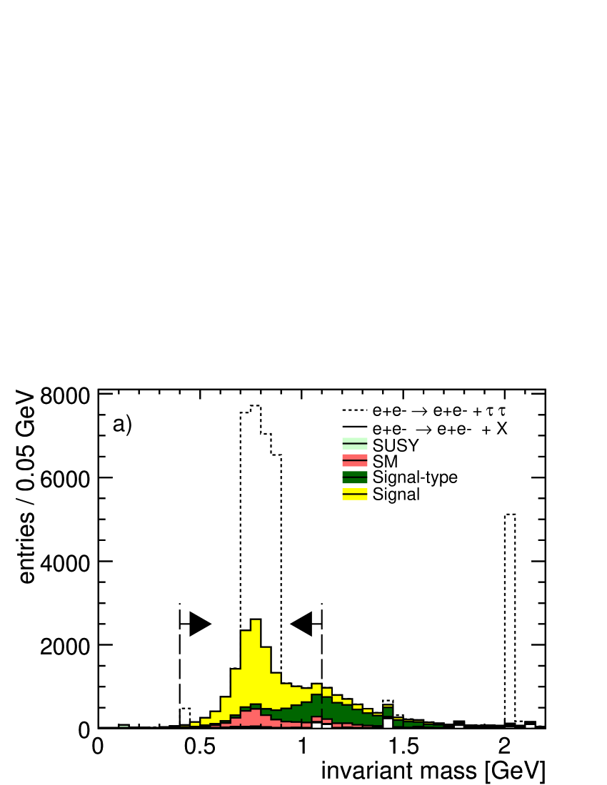
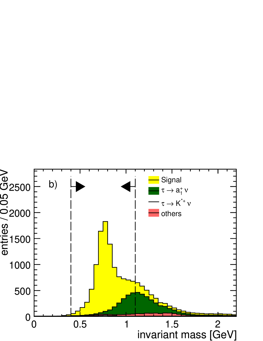
Figure 14: Distribution of $M_{jet}$ in the selected $\rho$ sample. a): Signal and all background: Medium light grey (yellow) histogram: Signal. Dark grey (dark green) histogram: Background from other decays of the $\tau$ from $\tilde{\tau}_{1}$. Light grey (light green) histogram: Background from other SUSY processes. Grey (red) histogram: Background from SM processes, except $\gamma\gamma$. Open dashed and solid histograms: Background from $\gamma\gamma\rightarrow\tau\tau$, and $\gamma\gamma\rightarrow X$. b): Signal and signal-type SUSY background, broken down by $\tau$ decay-mode.: Light grey (yellow) histogram: Signal. Dark grey (green) histogram: Background from $\tau\rightarrow a_{1}\nu_{\tau}$. Open histogram: Background from $\tau\rightarrow K\nu_{\tau}$. Grey (red) histogram: Background from other $\tau$ decays.

The signal decays were selected by demanding that the corresponding jet had $|\cos{\theta_{jet}}|<0.8$. The calorimeter-based PFOid algorithm was not used, because of the presence of two or more neutral clusters close to the track gives an unacceptably low efficiency for the signal. The measurement of $dE/dx$ in the TPC has no such problem, and was used to reject $\tau^{\pm}\rightarrow e^{\pm}\nu_{\tau}\nu_{e}$ (accompanied by bremsstrahlung photons) and $\tau^{\pm}\rightarrow K^{\pm}\pi^{0}\nu_{\tau}$. Finally, the mass of the jet should be around the mass of the $\rho$: $M_{jet}\in[0.4,1.1]~{}\mbox{${\mathrm{GeV}}$}$. Only about 7 % of the non-signal decays of the $\tilde{\tau}_{1}$ were misidentified, while 86 % of the signal decays still remained. Figure  14 shows the invariant mass spectrum of the selected events.

The final selection contained 8165 signal jets, 1991 from other decay modes of the $\tau$ in $\tilde{\tau}_{1}$$\tilde{\tau}_{1}$-events ($a_{1}$: 1602, $K^{*\pm}$: 131, all other 258), 1825 from jets in other SUSY channels, and 195 SM jets. In addition, the background from $\gamma\gamma$ processes was estimated to be 3000 jets, but the lack of statistics in the simulation made it difficult to asses this number with precision. Due to this, the background was estimated in a somewhat less sophisticated manner than for the $\pi$ channel. The distribution of $E_{\pi}/E_{jet}$ for the $\gamma\gamma$ before cuts was scaled down to correspond to the number of such events that survived all cuts, and this rescaled distribution was added to the background from other sources.

Similarly to the $\pi$ channel, an efficiency correction function, determined from signal-only simulation, was applied. Only the efficiency is assumed be dependent on the experimental situation, not the true spectrum. Therefore, and contrary to the case of the $\pi$ channel, the two steps (spectrum correction and efficiency determination) could be merged into one, directly yielding an efficiency-corrected model prediction:

$$dN/dR=N \left[\left(\frac{1-\mathcal{P}_{\tau}}{2}\right)^{2}f_{--}(R)+\left(\frac{1-\mathcal{P}^{2}_{\tau}}{2}\right)f_{+-}(R)+\right.$$

$$\left.\left(\frac{1+\mathcal{P}_{\tau}}{2}\right)^{2}f_{++}(R)\right]$$

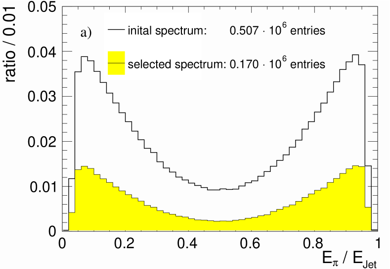
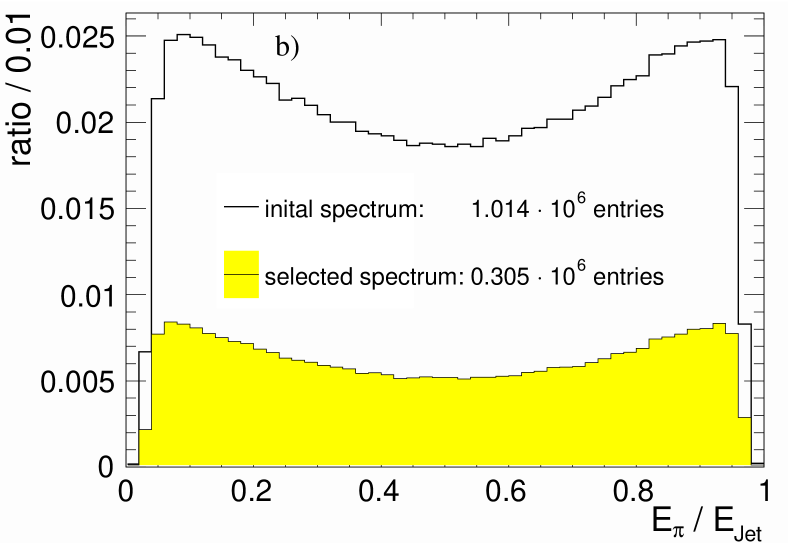
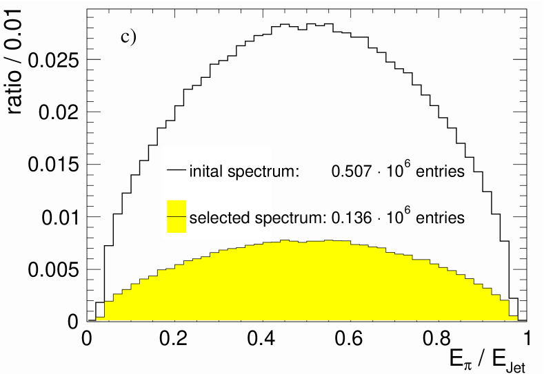
Figure 15: Distribution of $R=E_{\pi}/E_{jet}$ before (open histogram) and after event selection (grey (yellow) histogram). a): both $\tau$ leptons are right-handed. c): the $\tau$ leptons have opposite helicity. r): both $\tau$ leptons are left-handed.

The efficiency corrected spectra $f_{--}(R)$, $f_{+-}(R)$, and $f_{++}(R)$, correspond to the cases of the $\tau$ leptons being both of negative, of opposite, or both of positive helicity, respectively. These spectra were determined by fast simulation, see Fig. 15.

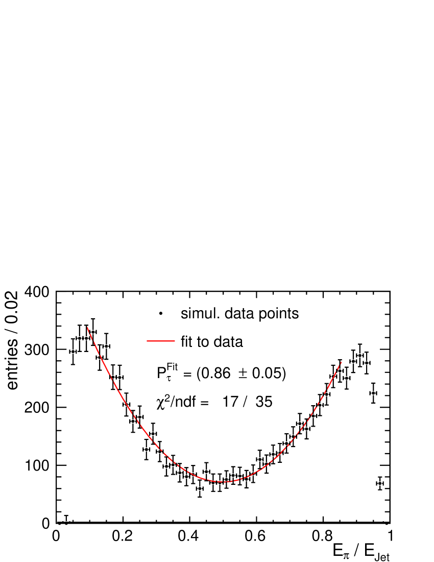
Figure 16: The distribution of $R=E_{\pi}/E_{jet}$ in the selected sample. The line shows the fitted efficiency and background corrected model.

The fast simulation was too optimistic, both in overall selection efficiency, and the efficiency for low and high $R$. Hence the fit was restricted to $R$ between 0.1 and 0.85, where the shape between full and fast simulation agreed, and the efficiency was scaled down equally for all polarisation configurations so that it agreed with the full simulation value. The observed spectrum was then fitted, with $N$ and $P_{\tau}$ as parameters, see Fig. 16. The result for the polarisation, simultaneously fitted with the normalisation, was found to be $\mathcal{P}_{\tau}$ = $86\pm 5~{}\%$. Due to the large uncertainty on the $\gamma\gamma$ contribution, it was of little use to study the effects of the uncertainty of the much smaller SUSY background. Due to the near invariance of the $R$-distribution, the actual values of $M_{\tilde{\tau}_{1}}$ and $M_{\tilde{\chi}^{0}_{1}}$ are expected to have only a small impact on the results.

4 Summary and Conclusions

A study of $\tilde{\tau}$ channels in the SPS1a’ SUSY scenario based on a full simulation of the ILD detector at the ILC was presented.

The study was performed in the context of the detector performance studies in view of the ILD Letter of Intent. It was therefore based on a full detector simulation of all known SM processes and machine related backgrounds. All accessible channels of the SPS1a’ SUSY model were also simulated with the same procedures. The simulation was done assuming that the ILC was run at a centre-of-mass energy of 500 ${\mathrm{GeV}}$, delivering an integrated luminosity of 500 fb^-1 with the electron beam being 80% right polarised, and the positron beam being 30% left polarised. The nominal beam parameter set was used to simulate the beam energy spread and beamstrahlung.

The study has only considered $\tilde{\tau}$-pair production, other open channels were considered as SUSY background. This meant that the study was done without prior knowledge of $M_{\tilde{\chi}^{0}_{1}}$, so that it has concentrated on observables with low sensitivity to this parameter: spectrum endpoints, cross sections and polarisation. The expected effect of the uncertainty on $M_{\tilde{\chi}^{0}_{1}}$ on the determination of $M_{\tilde{\tau}}$ is nevertheless quoted in a parametric form.

Throughout, it has been assumed that the knowledge of the SM background will be good, so that any uncertainty on the average SM background is small compared to $\sqrt{N_{SM}}$ at the final stage of event selection. The same was assumed for the determination of the selection efficiency. The SUSY background, on the other hand, has been assumed to be poorly known. It has been assigned a relative error of 100 % in most of the cases studied, or at best to be equal to the Poisson fluctuations in signal-free control samples, typically of about the same size as the final signal sample under study.

The results on the study of the $\tilde{\tau}_{1}$ production for the spectrum endpoint, cross section, and $\tau$ polarisation were:

$$E_{\tau,max}= 42.11^{+0.14}_{-0.12}~{}\mbox{${\mathrm{GeV}}$}$$

$$\frac{\delta\sigma}{\sigma}= 3.1~{}\%$$

$$\mathcal{P}_{\tau}= 91\pm 6\pm 5~{}\mathrm{(bkg)}\pm 3~{}\mathrm{(SUSY~{}masses)}~{}\%~{}(\pi~{}\mathrm{channel})$$

$$\mathcal{P}_{\tau}= 86\pm 5~{}\%~{}(\rho~{}\mathrm{channel})$$

The endpoint could be used to determine $M_{\tilde{\tau}_{1}}$, and assuming $M_{\tilde{\chi}^{0}_{1}}$ has been measured to its nominal value ($97.7~{}\mbox{${\mathrm{GeV}}$}$) with an error of $\delta\mbox{$M_{\tilde{\chi}^{0}_{1}}$}$, it was found to be

$$\mbox{$M_{\tilde{\tau}_{1}}$}=107.73^{+0.03}_{-0.05}\pm 1.1\cdot\delta\mbox{$M_{\tilde{\chi}^{0}_{1}}$}~{}\mbox{${\mathrm{GeV}}$}~{}(\mathrm{endpoint}).$$

Also the cross section could be used to determine $M_{\tilde{\tau}_{1}}$. However, $E_{CMS}$= 500 ${\mathrm{GeV}}$ is much too far from the threshold for this to be competitive: In this case $\Delta(\mbox{$M_{\tilde{\tau}_{1}}$})/\mbox{$M_{\tilde{\tau}_{1}}$}$ would be 2.1% assuming a known mixing angle. This should be compared to $\Delta(\mbox{$M_{\tilde{\tau}_{1}}$})/\mbox{$M_{\tilde{\tau}_{1}}$}\sim 1~{}\permil$ from the end-point, with no assumption on the mixing angle.

The $\tau$ polarisation had a lower statistical error in the $\rho$ channel. However, this must be taken with caution, because there was a substantial amount of remaining SM background from $\gamma\gamma$ processes. Due to lack of simulation statistics, its contribution is poorly known.

The results on the study of the $\tilde{\tau}_{2}$ production for the spectrum endpoint and cross section were:

$$E_{\tau,max}= 151.0^{+2.0}_{-1.7}~{}\mbox{${\mathrm{GeV}}$}$$

$$\frac{\delta\sigma}{\sigma}= 4.2~{}\%$$

The endpoint value yielded

$$\mbox{$M_{\tilde{\tau}_{2}}$}=183^{+11}_{-5}\pm 18\cdot\delta\mbox{$M_{\tilde{\chi}^{0}_{1}}$}~{}\mbox{${\mathrm{GeV}}$}~{}(\mathrm{endpoint}).$$

For the $\tilde{\tau}_{2}$, $E_{CMS}$= 500 ${\mathrm{GeV}}$ is much more favourable for the determination of the mass from the cross section: the expected uncertainty was $\Delta(\mbox{$M_{\tilde{\tau}_{2}}$})/\mbox{$M_{\tilde{\tau}_{2}}$}$ = 2.4%, comparable to what could be obtained from the endpoint ($\sim$ 4%). Hence, the two could be combined to determine $M_{\tilde{\chi}^{0}_{1}}$, and the error was found to be 1.7 ${\mathrm{GeV}}$, similar to what was found in a separate analysis of $\tilde{\mu}_{\mathrm{L}}$ using the same simulated sample. However, this value assumes that the mixing angle is known.

The $\tilde{\tau}$ mixing angle has not been studied in this paper, because the most sensitive process for its determination - $\tilde{\tau}_{1}$$\tilde{\tau}_{2}$ production - should be studied below the $\tilde{\tau}_{2}$$\tilde{\tau}_{2}$ threshold to get a good signal to background ratio.

In comparison with previous studies, e.g. [3], [24] and [30], several new aspects have been taken into account here. Most prominently, the smearing of four-vectors with design goal resolutions has been replaced by a detailed simulation of the various sub-detectors, including support structures, read-out, coolling etc. Further realism has been added by including not only background from Standard Model processes and from beamstrahlung pairs, but also from other (non-signal) SUSY processes, not always taken into account in the previous studies. The consideration of these additional backgrounds required improvements of the $\tau$ reconstruction and of the signal selection cuts. After these efforts, the achieved precision on the $M_{\tilde{\tau}_{1}}$ and on the $\tau$ polarisation is comparable to previous studies. Precise quantitative comparisons would need to take into account the different SUSY scenarios and accelerator parameters which have been used. The expected precision for the $\tilde{\tau}_{2}$ mass and cross section have not been evaluated in either of the previous studies.

More specifically, a similar “SPS1a inspired” scenario with a slightly smaller mass difference between $\tilde{\tau}_{1}$ and $\tilde{\chi}^{0}_{1}$ has been studied in [24] with a fast simulation of the TESLA detector, i.e. a predecessor to ILD. With an integrated luminosity of 200 fb^-1 and a beam polarisation of $\mathcal{P}_{beam}(e^{+},e^{-})=(-0.6,+0.8)$ at a centre-of-mass energy of 400 ${\mathrm{GeV}}$, statistical precisions on $M_{\tilde{\tau}_{1}}$ of 140 ${\mathrm{MeV}}$, 100 ${\mathrm{MeV}}$ and 100 ${\mathrm{MeV}}$ have been achieved in the single $\pi$, $\rho$ and 3$\pi$ channels, respectively, excluding any contribution from the uncertainty of $M_{\tilde{\chi}^{0}_{1}}$. Combined, this corresponds to a precision of about 60 ${\mathrm{MeV}}$, quite similar to the ${}^{+30}_{-60}$ ${\mathrm{MeV}}$obtained here. The higher integrated luminosity assumed in the study presented here is compensated in [24] by a higher degree of positron polarisation and more optimal choice of the centre-of-mass energy, i.e. a higher cross section. Concerning the $\tau$ polarisation, a precision of 7 % has been achieved in [3] from the $\rho$ channel. There, a scenario with a significantly larger mass difference has been studied using the JLC fast detector simulation, assuming an integrated luminosity of 100 fb^-1, an electron beam polarisation of 0.95 and a centre-of-mass energy of 500 ${\mathrm{GeV}}$. In view of the differences in beam parameters and in the SUSY scenario, this is in good agreement with the results of this study.

Finally, it has to be pointed out that for many of the processes studied in this work, running the accelerator at $E_{CMS}$= 500 ${\mathrm{GeV}}$ is not optimal. An upcoming study will treat the entire SPS1a’ scenario as a whole, including how to partition the luminosity in an optimal way, and how to make use of non-$\tilde{\tau}$ channels to measure parameters - notably $M_{\tilde{\chi}^{0}_{1}}$ - that were found to be hard to access in the $\tilde{\tau}$ channels.

5 Acknowledgements

We would like to thank the simulation production team, in particular F. Gäde, S. Aplin, J. Engels and I. Marchesini, for their great effort to produce the large samples of events used in this work. We would also like to thank T. Barklow for producing the generated input files for the SM backgrounds. The help from Z. Wa̧s in interfacing TAUOLA with Whizard was much appreciated.

We acknowledge the support of the DFG through the SFB (grant SFB 676/1-2006) and the Emmy-Noether program (grant LI-1560/1-1).

References

- [1] J. A. Aguilar-Saavedra & al., Eur. Phys. J. C46 (2006) 43.
- [2] ILD Concept Group, The International Large Detector — Letter of Intent, (DESY-09-087), http://www.ilcild.org/documents/ild-letter-of-intent/LOI.pdf.
- [3] M. M. Nojiri, K. Fujii, T. Tsukamoto, Phys. Rev. D54 (1996) 6756.
- [4] Z. Zhang, in LCWS 2004, Proceedings (2004) 957, arXiv:hep-ph/0411035; M. Berggren & al., arXiv:hep-ph/0406010 (2004).
- [5] E. Boos & al. Eur. Phys. J C30 (2003) 395.
- [6] R. Barbieri & al., Phys. Lett. B119 (1982) 343; A. H. Chamseddine, R. Arnowitt, P. Nath, Phys. Rev. Lett. 49 (1982) 970; R. Arnowitt, A. H. Chamseddine, P. Nath, Phys. Rev. Lett. 50 (1983) 232; L. Ibañez, Phys. Lett. B118 (1982) 73; H. P. Nilles & al., Phys. Lett. B120 (1983) 346; L. Hall, J. Lykken, S. Weinberg, Phys. Rev. D27 (1983) 2359.
- [7] C. F. Berger & al., JHEP 0902 (2009) 23.
- [8] O. Buchmüller & al. Eur. Phys. J C64 (2009) 391.
- [9] W. Porod, Comput. Phys. Commun. 153, (2003) 275.
- [10] M. M. Nojiri, Phys. Rev. D51 (1995) 6281.
- [11] S. Agostinelli & al., Nucl. Instr. Meth. A 506 (2003) 250.
- [12] G. Musat, in LCWS 2004, Proceedings (2004) 437; P. Mora de Freitas, in LCWS 2004, Proceedings (2004) 441.
- [13] M. Kobayashi & al. Nucl. Instr. Meth. A581 (2007) 265.
- [14] M. Hauschild, private communication.
- [15] W. Kilian & al., arXiv:0708.4233 [hep-ph].
- [16] S. Jadach & al., Comput. Phys. Commun. 76 (1993) 361.
- [17] D. Schulte, PhD Thesis, DESY/Universität Hamburg, TESLA 1997-08 (1997).
- [18] O. Wendt & al., Pramana 69, (2007) 1109.
- [19] P. Billoir, Nucl. Instr. Meth. A225 (1984) 352.
- [20] M. A. Thomson, AIP Conf. Proc.896 (2007) 215.
- [21] S. Catani & al., Phys. Lett. B269 (1991) 432.
- [22] J. Abdallah & al. (DELPHI collaboration), Eur. Phys. J. C31 (2004) 421.
- [23] D. Decamp & al. (ALEPH Collaboration), Phys. Rept. 216 (1992) 253.
- [24] H.-U. Martyn, arXiv:hep-ph/0408226, (2004).
- [25] N. d’Ascenzo, PhD Thesis DESY/Universität Hamburg thesis-2009-004, (2009).
- [26] C. Rimbault & al. in LCWS 2007, Proceedings (2007).
- [27] The ILC Collaboration, International Linear Collider Reference Design Report 2007 ILC-REPORT-2007-001, (2007).
- [28] K. Hagiwara & al. Phys. Lett. B235 (1990) 198.
- [29] P. Schade, PhD Thesis DESY/Universität Hamburg thesis-2009-040, (2009).
- [30] V. Khotilovich & al. Phys. Lett. B618 (2005) 182.
- [31] H.-U. Martyn, arXiv:hep-ph/0406123, (2004).