pubList of Publications

e © 2009 Martin Thøgersen
Department of Physics and Astronomy
Aarhus University
Ny Munkegade, Bldg. 1520
DK-8000 Aarhus C
Denmark
Phone: +45 26 70 22 43
Email: martint@phys.au.dk

1st edition, July 2009.
Online version and bibliography: http://www.martint.dk/thesis

Cover image: Illustration of a Bose-Einstein condensate, bringing together the few-body concepts of Efimov states and Borromean binding.
Central image: NIST/JILA/CU-Boulder, 1995 (public domain). Left image: B. D. Esry and C. H. Greene, Nature, 440 (2006) 289. Top image: Public domain, GPL.

Layout and typography chosen and implemented by the writer.
Font: Computer Modern, 11pt.
Typesetting done with LaTeX 2ε, BibTeX and the report class.
Used packages: babel, graphicx, amssymb, amsmath, fancyhdr, fixme, tikz, xxcolor, multibib, caption, glossary, threeparttable, url, rotating
Figures are made with Gnuplot 4.2 and TikZ/PGF.
Printed by SUN-Tryk, Aarhus University.

This dissertation has been submitted to the Faculty of Science at Aarhus University, Denmark, in partial fulfillment of the requirements for the PhD degree in physics. The work presented has been performed under the supervision of Ass. Prof. Dmitri Fedorov and Sen. Ass. Prof. Aksel S. Jensen. The work was carried out at the Department of Physics and Astronomy in Aarhus during the period August 2005 to July 2009. The group of Brett D. Esry at the Physics Department, Kansas State University, Manhattan, KS, USA, is also acknowledged for its hospitality during the spring of 2008.

Outline

This thesis describes theoretical investigations of universality and finite-range corrections in few- and many-boson systems. The major part of this work concerns ultra-cold trapped atomic gases, but some of the results and methods may be applicable to small molecules, and nuclei too.

In the introductory chapter 1 we briefly describe some of the basic concepts and phenomenology used in this dissertation such as universality, Bose-Einstein condensation, Efimov physics, and Borromean binding. The typical experimental systems of interest are also described.

Chapter 2 reviews the relevant theoretical background and methods for few-body systems as well as mean-field models for condensates. The numerical procedures we implement are also described. This gives a common background for the rest of the dissertation. The main chapters 3–8 can be read almost independently, but they often refer back to chapter 2.

In chapter 3 we investigate universal finite-range corrections to Efimov physics in three-boson systems. Connections to Borromean binding are made. We also describe the effects of putting the system in a finite trap. Chapter 4 continues this line by investigating the conditions for Efimov physics, in particular for large effective range. The content of chapter 3 and 4 was published in [TFJ08c, TFJ⁺09], but new material is also presented. (See page 1 for a list of publications.)

In chapter 5 we show the existence of a many-body Efimov effect based on two-body correlations. The features of the effect and experimental signatures are discussed. This chapter is based on [TFJ08a, FJT08] as well as some new results.

In chapter 6 we numerically consider trapped few-boson systems of order 10–30 particles including two-body correlations. Condensate-type states are identified. We investigate energies and correlations for these condensate states and discuss possible experimental signatures. Appendix A and B contains some technical details used in this chapter. The content of this chapter is composed of selected material from [TFJ07, TFJ08b, FJT08, JKTF07].

Chapter 7 approaches the question of effective range corrections in condensates from the mean-field point of view. A modified Gross-Pitaevskii equation is combined with a higher-order Feshbach resonance model. Effects on stability and decay mechanisms are predicted. In chapter 8 we continue the mean-field analysis of condensates. We present the Thomas-Fermi approximation in the case of higher-order interactions. Some details are found in appendix C. Chapter 7 and 8 are based on [TZJ09, ZT09b, ZT09a].

Conclusions and outlook are given in chapter 9. The back-matter contains appendices and the bibliography.

The results presented in [FJT⁺09] do not fit in the line of this thesis and is omitted.

Online information: This dissertation is available online at the address http://www.martint.dk/thesis, as well as on the arXiv preprint server. The bibliography for the thesis is also available on the above address, including abstracts and direct (doi) links to all referenced articles. This will hopefully be useful for the reader.

pub-thogersen08-3,pub-thogersen09a,pub-thogersen08-2, pub-fedorov08-1,pub-fedorov09-1,pub-thogersen07, pub-thogersen08-1, pub-fedorov08-1, pub-jensen07, pub-thogersen09b, pub-zinner09a, pub-zinner09b

Chapter 1 Introduction

Universality or model-independence is desirable in theoretical and experimental physics because the scope becomes broader and the applications more transparent and flexible. Universality generally refers to systems determined by only a few large-distance parameters, implying that they become independent of the specific short-range interactions and structure. Thus, once theoretical formulations are established they can be applied to a wide range of fields, e.g. nuclear, atomic, and molecular physics. Much effort has therefore been devoted to extract universal features in many branches of physics.

1.1 Ultra-Cold Atomic Gases

One system in which universality can be found is Bose-Einstein condensates (BEC) where cold massive bosons occupy the same quantum-mechanical state. The BEC concept was proposed almost a century ago [Ein24], but remained an elusive goal for atomic gas experiments for many years. The quest for this cold grail was motivated by several factors. The idea of a macroscopic number of particles in the same single-particle ground state is simple, elegant, and easy to grasp. Also, it is direct evidence of quantum mechanics and particle-wave duality on a macroscopic scale.

Since the experimental realization of the first BEC atomic ⁸⁷Rb two decades ago [AEM⁺95] the field of ultra-cold atomic gases has picked up speed. Bose-Einstein condensation has now been achieved for most of the alkali gases in numerous experimental groups, typically with ⁷Li, ²³Na, ³⁹K, ⁴¹K, ⁸⁵Rb, ⁸⁷Rb, and ¹³³Cs [PS02]. In the wake of the BEC milestone [AEM⁺95] a tremendous variety of experiments has been realized [BDZ08, GPS08]. This includes the interference between two condensates proving full coherence [ATM⁺97], structured arrays of quantized vortices in rotating condensates [ASRVK01], and propagating solitons and sound-like waves [PS03]. Besides standard (harmonic) traps, numerous experiments have been performed with different external confinement, including one- and two-dimensional gases and optical lattices with e.g. Mott-insulating phases [BDZ08]. Experiments with ultra-cold fermions have also given rise to new physics, e.g. BEC-BCS crossover and super-fluidity have been realized [GPS08]. Moreover, it is possible to produce cold gases with a wide range of mixed bosonic and fermionic species [SZS⁺04, IGO⁺04]. Production of bosonic gases with a small definite number of atoms is also in progress [DRN07].

Currently, one of the most important experimental tools for ultra-cold gases is the use of Feshbach resonances [KGJ06, CGJT09], which are found in virtually any atomic system. This allows for arbitrary tuning of atomic scattering lengths (i.e. low-energy interaction strengths) by varying an external magnetic field. Tunable scattering lengths have been a key ingredient for controlling the production, macroscopic stability, and decay of condensates [DGPS99]. The Feshbach resonance method also allows for production of weakly bound diatomic molecules (shallow dimers) [KGJ06, CGJT09].

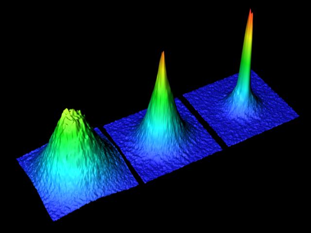
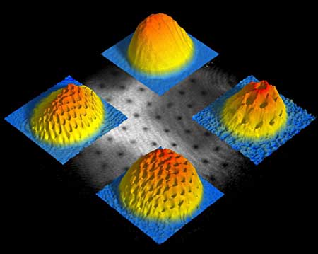
Figure 1.1: Experimental realization of Bose-Einstein condensation in trapped alkali gases. Left: The characteristic “spike” of condensed ⁸⁷Rb atoms emerges from the thermal cloud as the temperature is lowered below a critical value. Right: A rotating ²³Na BEC with vortices arranged in a highly ordered structure. From ETH Zurich (2002) and MIT (2001) [ASRVK01].

From the perspective of universality the scattering length is the decisive parameter for ultra-cold gases. Most features of the above experiments can be understood in terms of this parameter alone. This simplifies the theoretical descriptions immensely and makes the interpretations of the physical effects extremely sharp and clear. Most of the theoretical models for condensates are based on some sort of mean-field approximation with a contact interaction proportional to the scattering length. This means that all high-energy effects are integrated out and short-range model-dependent correlations are neglected. Thus it gives simple models which by definition are strictly universal.

When such universal models are used it is of course essential to know the precise “window” where the results can be applied to experiments. In many realistic cases this window is in fact very narrow. It is therefore important to know the qualitative significance of higher-order effects at the border of this window. The higher-order effects may ultimately be expressed in terms new model-independent parameters, but can also be strictly non-universal.

1.2 Few-Body Systems and the Efimov Effect

Another long-standing prediction of universality is the Efimov effect, which was presented in the early 1970s [Efi70, Efi71, AN71, AN72, Efi73] and has been discussed thoroughly since [FRS79, FJ93, FJR94, AFT97, NFJ99, FJ01b, NFJG01, BH06]. It is an anomalous effect which occurs in neutral three-body systems when at least two of the underlying subsystems have resonant $s$-wave interactions, i.e. a diverging scattering length (or at least much larger than the range of the physical force). This corresponds to the subsystems being close to the threshold for binding. Under these conditions an exceptional sequence of infinitely many geometrically spaced three-body bound states occurs, with an accumulation point at zero energy. Moreover, the ratio between the energies is a universal constant depending only on the mass ratios and the particle statistics. For three identical bosons the famous ratio is [NFJG01]

$$\frac{E_{T}^{(n)}}{E_{T}^{(n+1)}}=\textrm{e}^{2\pi/s_{0}}\simeq 515.0\;.$$ (1.1)

We emphasize that this specific scaling factor is independent of the mass, and that the same effect in principle can be found at all physical scales. The Efimov states have large sizes which are also geometrically spaced with ratios $515.0^{1/2}=22.7$, and lie outside the classically allowed region.

The effect was initially proposed by V. Efimov within the field of nuclear physics and has been searched for over many years in nuclei – unfortunately this search has been futile. The only possible three-body candidate without Coulomb interactions is two neutrons and a (positively charged) core. The possible resonant $s$-wave interactions should then be between each of neutrons and the core. Such three-nucleon systems, called two-neutron halos, do in fact exist. Common examples are ⁶He ($\alpha+n+n$) and ¹¹Li (⁹Li$+n+n$) [JRFG04] where the essential degrees of freedom correspond to the core$+n+n$ structure. Unfortunately the heavy-light-light mass ratio gives an extremely large scaling factor (as compared to the already large factor in eq. (1.1)) [JF03]. Thus one can only hope for “accidental fine-tuning” of the neutron-core scattering length to see the Efimov effect. One of the few candidates is ²⁰C [AFT97, BH06]. The Efimov effect has also been searched for in atomic systems. There is a general theoretical consensus [LDD77, ELG96, EG06, NFJ98] that the first excited state of the atomic helium trimer ⁴He₃ is an Efimov state, although the experimental observation so far proved elusive [BKK⁺05].

Another concept closely related to the Efimov effect is Borromean binding. The phrase refers to atypical bound few-body systems where none of the individual subsystems are bound. This is often symbolized by the interlocked Borromean rings, see fig. 1.2. Borromean systems are typically weakly bound with large spatial probabilities in classically forbidden regions. This implies that the structure is mainly determined by the binding energy alone, and are thus good universal candidates. The Efimov effect can be seen as a critical limit of Borromean binding: Here the two-body subsystems are exactly at the threshold but infinitely many bound three-body states exists. Examples of Borromean systems are the two-neutron halos ⁶He and ¹¹Li discussed above as well as ⁹Be ($\alpha+\alpha+n$) [JRFG04].

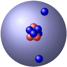
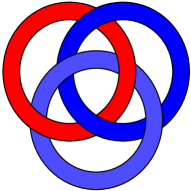
Figure 1.2: Left: Schematic two-neutron halo nucleus with the neutrons weakly bound to the core. Right: Interlocked Borromean rings: If one ring is removed the others fall apart. The name “Borromean” is historical and comes from the aristocratic Italian Borromeo family who used the rings in their coat of arms.

1.3 Efimov Physics in Atomic Gases

The obstacles for observing the Efimov effect in nuclei are three-fold: i) nuclei are electrically charged, ii) the are no methods for tuning the interactions externally so one must rely on accidental tuning, and iii) the remaining candidates have very unfortunate mass ratios. Instead, the approach of observing the Efimov effect indirectly via three-body recombination losses in ultra-cold atomic gases attract much attention currently. As compared to nuclei, atomic gases are very promising for several reasons: i) atoms are electrically neutral, ii) scattering lengths can be tuned by magnetic Feshbach resonances, and iii) by using different species with appropriate mass ratios (heavy-heavy-light) the universal scaling factor can be reduced. Concerning the last part, specific proposals for ultra-cold atomic gas mixtures were given in [DE06], for example the realized boson-fermion mixtures ²³Na-⁶Li [SZS⁺04] or ⁸⁷Rb-⁴⁰K [IGO⁺04], or even better ¹³³Cs-⁶Li or ⁸⁷Rb-⁶Li.

The basic idea for observing Efimov states using Feshbach resonances is to measure the bound state spectrum indirectly. When the scattering length is tuned around large values, a series of resonance and interference effects occurs in the three-body recombination rate [EG06, BH06]. These features are located at critical scattering lengths with the same scaling factor as the Efimov sequence, i.e. 22.7 for identical bosons. The first experimental indications of such features has been found recently in cold ¹³³Cs gases [KMW⁺06, KFM⁺09]. Also, a universal trimer state is reported in a three-component ⁶Li Fermi gas [WLO⁺09]. Recent theoretical [DvSG09, vSDG09] and experimental [FKB⁺09] work indicate the existence of a universal four-body effect where an atom is weakly bound to an Efimov trimer.

The phrase “Efimov physics” was introduced recently in the context of atomic gases and Feshbach resonances [DE05], but is now used more and more frequently. We will adopt this phrase to the extent possible: By “Efimov effect” we refer to the infinite accumulation of trimers states at the threshold, while by “Efimov physics” we mean the broader concept in cold gases using Feshbach resonances and recombinations loss for observing the Efimov effect and related features.

The experiments performed until now strongly indicate that individual features of Efimov states have been found. However, the results are yet not conclusive [LKJ07]. Definite evidence requires two, or even better a whole sequence, of the states with the correct relative scaling to be observed. The universal window is still quite small and experimental control is not at its final level yet. Theoretical physics can help at this point by predicting quantitatively the regions where universality occurs, as well as the corrections at the border of these regions.

The subject of universality in atomic gases will face many new challenges during the next decades. In the most recent review on universality in few-body systems [BH06], three subjects were marked as the frontiers of this field: The $N$-body problem for $N\geq 4$, effective range corrections, and large $p$-wave scattering length. These issues are clearly within reach in ultra-cold gases and indicate a promising future.

1.4 Angle of this Thesis

In this dissertation we carry out theoretical investigations of universality and its limits in few- and many-boson systems. We focus on ultra-cold trapped atomic gases, but strive to present the results in universal terms and via model-independent parameters. Thus, much of the work may hopefully be used or continued in other areas of physics.

We will investigate effective range corrections and trap effects to Efimov physics, as well as the limits of the universal predictions. Next we investigate the possibility of an Efimov effect in $N$-body systems. We also consider trapped BEC-like states from the few-body level, where we will be concerned with model-independence and two-body correlations. The approach to answer these questions will be from the pure few-body level, keeping in mind only to include the degrees of freedom needed for physical relevance. Finally, we approach Bose-Einstein condensates from the angle of standard mean-field theory, but with higher-order interaction terms included.

Note added.

The observation of an Efimov spectrum in an ultra-cold gas has just been published [ZDD⁺09], giving the first definite proof of the universal scaling factors. This happened at the very final stage of writing this dissertation (I, the author, only became aware of the results a few days before handing in the thesis). To keep the chronological order, no contents or conclusions have been modified at all. A more elaborate note is found in the summary chapter.

Chapter 2 Theoretical and Numerical Background

In this chapter we consider some of the theoretical background for few-body systems. For the two-body systems we discuss basic universal behavior, as well as some results on Feshbach resonances, atomic interactions, and model potentials. Specifically we discuss the large effective range. For the three-body systems we derive the Efimov effect in the hyper-spherical adiabatic approximation and explain experimental consequences for recombination rates. We also briefly review some mean-field concepts. Finally we describe the stochastic variational method which is one of the main numerical tools for our work.

2.1 Two-Body Systems

2.1.1 Low-Energy Scattering

Let us briefly review some relevant low-energy concepts for two-body scattering and bound states. We will be concerned with the limit where where only the lowest partial waves, $l=0$, contribute [BJ03]. Here the scattering can be described by the radial Schrödinger equation

$$\left(\frac{\partial^{2}}{\partial r^{2}}-U(r)+k^{2}\right)u(r)=0,$$ (2.1)

where $r=|\mbox{\boldmath$r$}_{1}-\mbox{\boldmath$r$}_{2}|$ is the inter-particle distance, $U(r)=2mV(r)/\hbar^{2}$ is the two-body interaction, $m$ the particle mass, $u(r)=R(r)r$ the $s$-wave radial function, $k=\sqrt{2mE}/\hbar$ the wave number, and $E$ the relative energy. The asymptotic behavior

$$u\sim\sin(kr+\delta(k))$$ (2.2)

defines the $s$-wave phase shift $\delta(k)$ as function of the incident energy. The scattering amplitude $f(k)$, defined as the ratio of outgoing spherical waves and ingoing plane waves, is in this case spherically symmetric and related to the phase shift by

$$f(k)=\frac{1}{k\cot\delta(k)-ik}.$$ (2.3)

The total cross-section is then given by $\sigma=8\pi|f(k)|^{2}$ for identical bosons. For small energies one traditionally employ the effective range expansion for the phase shift,

$$k\cot\delta(k)=-\frac{1}{a}+\frac{R_{e}}{2}k^{2}+\dots,$$ (2.4)

where $a$ is the scattering length and $R_{e}$ is the effective range.

The poles of the scattering amplitude $f(k)$ defines the bound states, virtual states, and resonances for the two-body problem. The bound states are located on the positive imaginary axis in the complex $k$-plane, i.e. $k=i\kappa$, $\kappa>0$. The binding wave number $\kappa$ is then determined by the equation,

$$i\kappa\cot\delta(i\kappa)+\kappa=0.$$ (2.5)

The corresponding energy is given by

$$E_{D}=\frac{\hbar^{2}k^{2}}{m}=-\frac{\hbar^{2}\kappa^{2}}{m},$$ (2.6)

where the binding energy is $B_{D}=|E_{D}|$. Contrary to the bound states, the virtual states (or anti-bound states) are located on the negative imaginary $k$-axis, i.e. $k=i\kappa$, $\kappa<0$. The corresponding energy is also real and negative,

$$E_{V}=\frac{\hbar^{2}k^{2}}{m}=-\frac{\hbar^{2}\kappa^{2}}{m},$$ (2.7)

however, the pole is located on the second Riemann sheet, and can thus only be measured indirectly via analytic continuation of the cross section.

2.1.2 Universal Bound States

Using only the lowest scattering length term in the effective range expansion of eq. (2.4) and inserting in eq. (2.5), we find a single pole with wave number $\kappa=1/a$. For $a>0$ this gives a bound state with energy

$$E_{D}=-\frac{\hbar^{2}}{ma^{2}},$$ (2.8)

which holds when the scattering length is much larger than the inter-atomic potential range, $r_{0}$. In atomic physics such a weakly bound two-body state is often referred to as a shallow dimer. This type of state is universal, or model-independent, in the sense that it depends only on the scattering length and not the details of the short-range potential: The major part of the wave-function is an exponential tail located outside $r_{0}$, which is an essential example of universality. The state can also be described in a zero-range model where the usual boundary condition $u(0)=0$ is replaced by

$$\left.\frac{1}{u}\frac{\partial u}{\partial r}\right|_{r=0}=\left.k\cot\delta(k)\right|_{k\to 0}=-\frac{1}{a}.$$ (2.9)

This leads to the wave number $\kappa=1/a$ and exponentially decreasing wave-function $u\sim\exp(-r/a)$.

If we also include the effective range in eq. (2.4), the binding wave number is determined by $R_{e}\kappa^{2}/2-\kappa+1/a=0$. This gives

$$\kappa=\frac{1}{R_{e}}\left(1-\sqrt{1-2R_{e}/a}\right),$$ (2.10)

where we have chosen the negative root. The state corresponding to the positive root is unphysical, since it is strongly bound with energy $E\sim\hbar^{2}/(mR_{e}^{2})$ comparable to the potential depth [BH06]. Thus for $a>0$ we have a bound dimer with energy

$$E_{D}=-\frac{\hbar^{2}}{mR_{e}^{2}}\left(1-\sqrt{1-2R_{e}/a}\right)^{2}.$$ (2.11)

The virtual state energy $E_{V}$ is given by the same expression for $a<0$. Equation (2.11) holds when the higher-order shape terms in the effective range expansion are negligible. Expanding it to lowest order in $R_{e}/a$ gives

$$E_{D}=-\frac{\hbar^{2}}{ma^{2}}\left(1+\frac{R_{e}}{a}+O(\frac{R_{e}^{2}}{a^{2}})\right),$$ (2.12)

which is then a small correction to eq. (2.8).

2.1.3 Feshbach Resonances

Feshbach resonances is one of the most important experimental tools for ultra-cold atomic gases, see [CGJT09] for a recent review. These resonances allows for arbitrary tuning of scattering lengths, in particular the $s$-wave scattering length which is relevant for our purpose. This has been a major key for controlling macroscopic stability and decay of condensates [DGPS99], and for creating shallow molecular dimers [CGJT09].

In the zero-range approximation, the scattering length of a Feshbach resonance can be described by the phenomenological magnetic field dependent expression

$$a(B)=a_{bg}\left(1-\frac{\Delta B}{B-B_{0}}\right).$$ (2.13)

Here $a_{bg}$ is the background scattering length away from resonance, $B_{0}$ is the position of the Feshbach resonance and $\Delta B$ the width. Experimentally, these resonance parameters are usually determined indirectly via peaks in the loss rate of condensates.

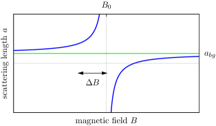
Figure 2.1: Scattering length $a(B)$ for the Feshbach resonance model eq. (2.13) as function of magnetic field $B$. The resonance is centered around $B_{0}$ with width $\Delta B$ and has background scattering length $a_{bg}$.

The phenomenological behavior in eq. (2.13) can be reproduced in various models, a common example is the two-channel model described in [PS02]. In this model the resonance width $\Delta B$ turns out to be proportional to the matrix element connecting the open and closed channels that overlap in energy and cause the resonant behavior, see fig. 2.2.

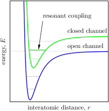
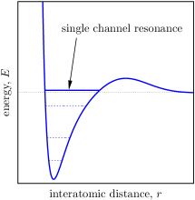
Figure 2.2: Left: Schematic representation of a Feshbach resonance. A bound state of the closed channel has energy close to the (zero) incoming energy of the open channel. The relative position of the channels can be changed by an external magnetic field, thereby tuning the coupling. Right: A schematic (shape) resonance of a single-channel model. The Feshbach resonance can be modeled by a shape resonance if the elastic (open-open channel) scattering is the only contribution.

The scattering length, eq. (2.13), is obtained when a two-channel model is reduced to an effective single-channel model. The related effective range of the effective single-channel zero-range model is determined from the resonance width as (see e.g. [BJK05]),

$$R_{e0}=-2\frac{\hbar^{2}}{m\Delta\mu\Delta Ba_{bg}},$$ (2.14)

where $\Delta\mu$ is the difference between the magnetic moments in the open and closed channel. This result holds on-resonance, i.e. near $|a|=\infty$. In terms of common experimental units the effective range reads

$$R_{e0}=\frac{-5.16\cdot 10^{6}a_{0}}{\left(\tfrac{m}{m_{u}}\right)\left(\tfrac{a_{bg}}{a_{0}}\right)\left(\tfrac{\Delta\mu}{\mu_{B}}\right)\left(\tfrac{\Delta B}{G}\right)},$$ (2.15)

where $a_{0}$ is the Bohr radius, $m_{u}$ is the unified atomic mass unit, $\mu_{B}$ the Bohr magneton, and $\Delta B$ is measured in Gauss. The effective range is always negative but can be arbitrarily large for narrow resonances. This is consistent with our observations for the zero-range limit of finite-range potentials, see below.

The effective range, eq. (2.14), is constant (independent of magnetic field strength, $B$) and only holds near $|a|=\infty$. In chapter 7 we derive the more general $B$-dependent effective range,

$$R_{e}=R_{e0}\left(1-\frac{a_{bg}}{a(B)}\right)^{2}.$$ (2.16)

2.1.4 Atomic Interactions and Model Potentials

van der Waals Interaction

The real atomic potential between neutral atoms can in the Born-Oppenheimer approximation mainly be described by a short-range and a long-range part. The short-range repulsive core arises from the overlapping electron clouds, while the attractive long-range van der Waals interaction is due to the polarizability of the electron clouds. Asymptotically this van der Waals tail goes as

$$V(r)\simeq-\frac{C_{6}}{r^{6}}+O\left(\frac{1}{r^{12}}\right).$$ (2.17)

For ultra-cold gases, where the relative momentum between the atoms is small, this is the dominating part of the interaction. The $C_{6}$ coefficient defines the van der Waals length

$$l_{vdW}=\left(\frac{mC_{6}}{\hbar^{2}}\right)^{1/4},$$ (2.18)

which is the typical interaction length scale between neutral atoms. Examples of $l_{vdW}$ are $44.93a_{0}$ for ²³Na and $82.58a_{0}$ for ⁸⁷Rb [CGJT09]. The effective range for the single-channel van der Waals interaction can be estimated to $R_{e}\simeq 1.39l_{vdW}$ for $a\gg l_{vdW}$ [CGJT09].

Model Potentials

Low energy scattering can be described by model potentials of finite range. Typical choices are the finite square well or a van der Waals tail with a hard core which can be solves analytically. For example, the square well has scattering length and effective range

$$\frac{a}{r_{0}}=1-\frac{\tan s}{s},\qquad\frac{R_{e}}{r_{0}}=1-\frac{1}{3}\left(\frac{r_{0}}{a}\right)^{2}-\frac{1}{s^{2}}\frac{r_{0}}{a},$$ (2.19)

in terms of the finite range $r_{0}$ and dimensionless depth $s=r_{0}\sqrt{mV_{0}}/\hbar>0$. Each time a bound state is at the threshold, $a$ diverges ($s=\pi/2+n\pi$) and the effective range equals the finite range $R_{e}=r_{0}$. When $a\to 0$ the effective range diverges as $-1/a^{2}$. The scattering length and effective range for the van der Waals tail ($-C_{6}/r^{6}$ for $r>r_{0}$) with hard core ($\infty$ for $r<r_{0}$) is found in [BH06].

Another common choice is the Gaussian potential

$$V(r)=V_{0}\exp(-r^{2}/r_{0}^{2}),$$ (2.20)

which we will use later for numerical calculations. The scattering length have features similar to the square well, but the effective range is always positive for the attractive case, see fig. 2.3.

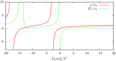
Figure 2.3: Scattering length and effective range for the Gaussian interaction, eq. (2.20), in units of the range $r_{0}$. The first bound state occurs at $V_{0}=-2.68\hbar^{2}/(mr_{0}^{2})$.

Feshbach resonances can also be modeled by single-channel potentials. This is of course only possible if the energy is low and elastic scattering is considered. The model potential should have the same low-energy phase shift as the real Feshbach resonance. The diverging scattering length can be be modeled by any potential, just by tuning a two-body bound state to zero energy. However, as we saw in eq. (2.16) the effective range for a Feshbach resonance can be very large and negative. Only certain single-channel model potentials can reproduce this.

In general the effective range of a finite-range potential is given by

$$R_{e}=2\int_{0}^{\infty}\left[v_{0}^{2}(r)-u_{0}^{2}(r)\right]\,\mathrm{d}r,$$ (2.21)

where $u_{0}$ is the zero-energy wave-function normalized asymptotically as $u_{0}\to 1-r/a$, and $v_{0}=1-r/a$ is the asymptotic solution extended to all $r$. When considering a potential of finite range $r_{0}$, we have $u_{0}=v_{0}$ in the outer region and the integral only runs to $r_{0}$. Performing the integration over $v_{0}^{2}$ and noting that the integral over $u_{0}^{2}$ is positive we get the bound [PC97]

$$R_{e}\leq 2r_{0}\left(1-\frac{r_{0}}{a}+\frac{r_{0}^{2}}{3a^{2}}\right).$$ (2.22)

In the resonant limit $a=\infty$, we find $R_{e}\leq 2r_{0}$, in particular the effective range must be negative if we also approach the zero-range limit. We note that the large negative effective range occurs when the amplitude of $u$ is considerably larger inside the potential as compared to the asymptotic value ($v_{0}=1$).

This means that to reproduce a large negative effective range with a single-channel finite-range potential we need to have a (shape) resonance around zero energy, see e.g. fig. 2.2. The simplest way to do this is by having an attractive inner region and a repulsive barrier. This could for example be the square well with a square barrier, which can be solved analytically [JNW06]. We instead consider the softer potential with barrier

$$V(r)=D\ \text{sech}^{2}\left(\chi\frac{r}{r_{0}}\right)+B\exp\left(-2(\chi\frac{r}{r_{0}}-2)^{2}\right),$$ (2.23)

which is shown in fig. 2.4. By tuning the depth of the pocket and height of the barrier we can make both $a$ and $|R_{e}|$ much larger than $r_{0}$. This leads to a large amplitude of the zero-energy wave-function $u_{0}$ inside the potential, as compared to the asymptotic region. In the limit $|a|\to\infty,R_{e}\to-\infty$ all probability is located inside the potential. This means that universal features of the two-body problem can be lost for $R_{e}\to-\infty$ even within the normal universal limit of large scattering length. We investigate this point for the three-body Efimov effect in chapter 4.

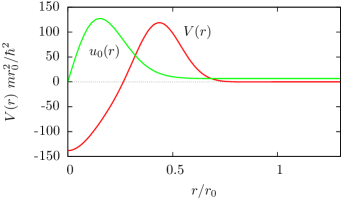
Figure 2.4: Soft two-body potential $V$ with barrier, eq. (2.23). The parameters $D=-138.27$, $B=128.49$ (in units $\hbar^{2}/(mr_{0}^{2})$), and $\chi=4.6667$ are tuned to give large scattering length $a=556.88$ and large negative effective range $R_{e}=-142.86$. The zero-energy wave-function $u_{0}(r)$ (arb. units) has large amplitude inside the barrier.

In conclusion, when we talk about effective range it means higher-order in the two-body scattering dynamics, i.e. the $k^{2}$ term of the phase shift expansion eq. (2.4). It can either be related to the finite range of a single-channel model potential (such as the van der Waals interaction) or the higher-order term of a coupled-channel Feshbach resonance, eq. (2.16). However, large effective range (compared to the interaction range $r_{0}$) can only occur near a Feshbach or shape resonance, and must be negative in this case.

2.2 Three-Body Systems

We now describe the three-body problem with the hyper-spherical adiabatic approximation. We consider the zero-range limit with a Faddeev-type decomposition and appropriate boundary conditions to derive the effective hyper-radial potential responsible for the Efimov effect. Applications and experiments are outlined.

2.2.1 Hamiltonian and Coordinates

Let us first describe the hyper-spherical adiabatic approximations, details can be found in [NFJG01, FJ01b]. We consider the three-body system with the center-of-mass (cm) Hamiltonian

$$\hat{H}=\hat{T}+\sum_{i<j}V(\mbox{\boldmath$r$}_{ij}),$$ (2.24)

where $\hat{T}$ is the kinetic energy operator in the center-of-mass frame and $V$ is the two-body interaction. We denote the vector from particle $j$ to $i$ by $\mbox{\boldmath$r$}_{ij}=\mbox{\boldmath$r$}_{i}-\mbox{\boldmath$r$}_{j}$, and the vector from the center-of-mass of the pair $(j,k)$ to particle $i$ by $\mbox{\boldmath$r$}_{i,(jk)}=\mbox{\boldmath$r$}_{i}-(\mbox{\boldmath$r$}_{j}+\mbox{\boldmath$r$}_{k})/2$. In the equal mass system the Jacobi coordinates $(\mbox{\boldmath$x$}_{i},\mbox{\boldmath$y$}_{i})$ for $i=1,2,3$ are defined as

$$\mbox{\boldmath$x$}_{i}=\frac{1}{\sqrt{2}}\mbox{\boldmath$r$}_{jk},\quad\mbox{\boldmath$y$}_{i}=\sqrt{\frac{2}{3}}\mbox{\boldmath$r$}_{i,(jk)},$$ (2.25)

where $\{i,j,k\}$ is a cyclic permutation of $\{1,2,3\}$, see fig. 2.5.

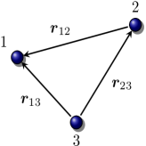
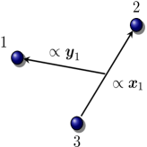
Figure 2.5: Relative coordinates $\mbox{\boldmath$r$}_{ij}$ and one set ($i=1$) of Jacobi-coordinates $\mbox{\boldmath$x$}_{1},\mbox{\boldmath$y$}_{1}$.

The six hyper-spherical coordinates $(\rho,\alpha_{i},\Omega_{xi},\Omega_{yi})$ are defined as

$$x_{i}=\rho\sin\alpha_{i},\quad y_{i}=\rho\cos\alpha_{i},$$ (2.26)

where $\rho\geq 0$ is the hyper-radius, $\alpha_{i}\in[0,\pi/2]$ is the hyper-angle, $\Omega_{xi}=\{\vartheta_{i},\varphi_{i}\}$ the angles describing the direction of $\mbox{\boldmath$x$}_{i}$, and similarly $\Omega_{yi}$ for $\mbox{\boldmath$y$}_{i}$. The hyper-radius

$$\rho^{2}=x_{i}^{2}+y_{i}^{2}=\frac{1}{3}(r_{12}^{2}+r_{13}^{2}+r_{23}^{2})$$ (2.27)

is independent of the chosen Jacobi-set and describes the average size of the three-body system. It is the only dimension-full coordinate of the hyper-spherical coordinates. All the angles are denoted together by $\Omega_{i}=(\alpha_{i},\Omega_{xi},\Omega_{yi})$. For fixed $\rho$, the hyper-angle $\alpha_{i}$ describes (together with $(\Omega_{xi},\Omega_{yi})$) the internal configuration. For $\alpha_{i}\sim 0$ particles $j,k$ are close to each other, and for $\alpha_{i}\sim\pi/2$ particle $i$ lies between $j$ and $k$, see fig. 2.6.

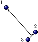
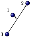
Figure 2.6: Two configurations with the same hyper-radius $\rho$ but different hyper-angles $\alpha_{1}$. Left: $\alpha_{1}\sim 0$. Right: $\alpha_{1}\sim\pi/2$.

The volume elements of the Jacobi and hyper-spherical coordinates are related by

$$\begin{split}&\,\mathrm{d}{\mbox{\boldmath$x$}_{i}}\,\mathrm{d}{\mbox{\boldmath$y$}_{i}}=\rho^{5}\,\mathrm{d}\rho\,\mathrm{d}\Omega,\\ &\,\mathrm{d}\Omega\equiv\sin^{2}\alpha_{i}\cos^{2}\alpha_{i}\,\mathrm{d}\Omega_{xi}\,\mathrm{d}\Omega_{yi}.\end{split}$$ (2.28)

The kinetic energy operator in hyper-spherical coordinates is given by

$$T=\frac{\hbar^{2}}{2m}\left(-\frac{\partial^{2}}{\partial\rho^{2}}-\frac{5}{\rho}\frac{\partial}{\partial\rho}+\frac{\hat{\Lambda}^{2}}{\rho^{2}}\right),$$ (2.29)

where the square of the grand angular momentum operator $\hat{\Lambda}$ is

$$\hat{\Lambda}^{2}=-\frac{1}{\sin 2\alpha_{i}}\frac{\partial^{2}}{\partial\alpha_{i}^{2}}\sin(2\alpha_{i})-4+\frac{\hat{l}_{xi}^{2}}{\sin^{2}\alpha_{i}}+\frac{\hat{l}_{yi}^{2}}{\cos^{2}\alpha_{i}}.$$ (2.30)

Here $l_{xi}^{2}$ and $l_{yi}^{2}$ are the angular momentum operators corresponding to $\mbox{\boldmath$x$}_{i}$ and $\mbox{\boldmath$y$}_{i}$. We only consider zero total angular momentum, i.e. $l_{xi}=l_{yi}=0$. Two different sets of Jacobi coordinates $i$ and $j$ are connected through the so-called kinematic rotation [NFJG01]

$$\begin{pmatrix}\mbox{\boldmath$x$}_{j}\\ \mbox{\boldmath$y$}_{j}\end{pmatrix}=\begin{pmatrix}-\cos\gamma_{ij}&\sin\gamma_{ij}\\ -\sin\gamma_{ij}&-\cos\gamma_{ij}\end{pmatrix}\begin{pmatrix}\mbox{\boldmath$x$}_{i}\\ \mbox{\boldmath$y$}_{i}\end{pmatrix}.$$ (2.31)

For three identical particles the “rotation angle” is $\gamma_{ij}=\sigma\{i,j,k\}\pi/3$, where $\sigma\{i,j,k\}$ is the sign of the permutation $\{i,j,k\}$. By calculating $\mbox{\boldmath$x$}_{i}^{2}$ from eq. (2.31) and using eq. (2.26), the different hyper-angles are then related by

$$\begin{split}\sin^{2}\alpha_{j}&=\cos^{2}\gamma_{ij}\sin^{2}\alpha_{i}+\sin^{2}\gamma_{ij}\cos^{2}\alpha_{i}\\ &-2\sin\gamma_{ij}\cos\gamma_{ij}\sin\alpha_{i}\cos\alpha_{i}\cos\theta_{i},\end{split}$$ (2.32)

where $\theta_{i}\in[0,2\pi]$ is the angle between $\mbox{\boldmath$x$}_{i}$ and $\mbox{\boldmath$y$}_{i}$. Using $|\cos\theta_{i}|\leq 1$ one can show that for a fixed hyper-angle $\alpha_{i}$ in the coordinate set $i$, the hyper-angle in set $j$ is restricted by

$$\left|\frac{\pi}{3}-\alpha_{i}\right|\leq\alpha_{j}\leq\frac{\pi}{2}-\left|\frac{\pi}{6}-\alpha_{i}\right|.$$ (2.33)

2.2.2 Hyper-Spherical Adiabatic Expansion

In the hyper-spherical adiabatic expansion one first solve the angular part ($\Omega$) of the Schrödinger equation for fixed $\rho$,

$$\left(\hat{\Lambda}^{2}+\frac{2m}{\hbar^{2}}\rho^{2}\sum_{i=1}^{3}V(\sqrt{2}\rho\sin\alpha_{i})\right)\Phi_{n}(\rho,\Omega)=\lambda_{n}\Phi_{n}(\rho,\Omega).$$ (2.34)

This gives a complete set of eigenfunctions $\Phi_{n}(\rho,\Omega)$ and corresponding eigenvalues $\lambda_{n}(\rho)$ as functions of $\rho$. We expand the total wave function as

$$\Psi=\sum_{n}\rho^{-5/2}f_{n}(\rho)\Phi_{n}(\rho,\Omega).$$ (2.35)

Inserting this into the full Schrödinger equation gives a coupled set of hyper-radial equations for the coefficients $f_{n}(\rho)$,

$$\left(-\frac{\partial^{2}}{\partial\rho^{2}}+\frac{2m}{\hbar^{2}}(V_{\textup{eff},n}(\rho)-E)\right)f_{n}(\rho)=\sum_{n^{\prime}\neq n}(2P_{nn^{\prime}}\frac{\partial}{\partial\rho}+Q_{nn^{\prime}})f_{n^{\prime}}(\rho),$$ (2.36)

where the effective hyper-radial potentials are

$$V_{\textup{eff},n}(\rho)=\frac{\hbar^{2}}{2m}\frac{\lambda_{n}(\rho)+15/4}{\rho^{2}}-Q_{nn},$$ (2.37)

and the non-adiabatic couplings are

$$\begin{split}P_{nn^{\prime}}(\rho)&=\left\langle\Phi_{n}(\rho,\Omega)\left|\frac{\partial}{\partial\rho}\right|\Phi_{n^{\prime}}(\rho,\Omega)\right\rangle_{\Omega},\\ Q_{nn^{\prime}}(\rho)&=\left\langle\Phi_{n}(\rho,\Omega)\left|\frac{\partial^{2}}{\partial\rho^{2}}\right|\Phi_{n^{\prime}}(\rho,\Omega)\right\rangle_{\Omega}.\end{split}$$ (2.38)

The brackets denote integration over $\Omega$. The angular wave-functions are normalized to unity for fixed $\rho$, i.e. $\langle\Phi(\rho,\Omega)|\Phi(\rho,\Omega)\rangle_{\Omega}=1$. The identity $P_{nn}=0$ also holds. In the strict adiabatic limit where all the off-diagonal coupling terms $P_{nn^{\prime}}$ and $Q_{nn^{\prime}}$ vanish, the hyper-radial equations, eq. (2.36), decouple.

2.2.3 Hyper-Angular Faddeev Decomposition

Let us first rewrite the angular equation eq. (2.34) as

$$\left(-\frac{\partial^{2}}{\partial\alpha_{i}^{2}}-\nu^{2}+\sum_{i=1}^{3}U(\alpha_{i})\right)(\sin(2\alpha_{i})\Phi)=0,$$ (2.39)

where the reduced interaction is $U(\alpha_{i})=\frac{2m}{\hbar^{2}}\rho^{2}V(\sqrt{2}\rho\sin\alpha_{i})$, the eigenvalue is $\nu^{2}=\lambda+4$, and we have omitted the subscripts $n$. We now split the hyper-angular wave-function into three identical Faddeev components,

$$\Phi(\alpha_{i})=\frac{\psi_{i}+\psi_{j}+\psi_{k}}{\sin(2\alpha_{i})},$$ (2.40)

which fulfill the three Faddeev equations

$$\left(-\frac{\partial^{2}}{\partial\alpha_{i}^{2}}-\nu^{2}\right)\psi_{i}+U(\alpha_{i})(\psi_{i}+\psi_{j}+\psi_{k})=0.$$ (2.41)

Adding these equations leads to eq. (2.39). The components $\psi_{i},\psi_{j},\psi_{k}$ have the same functional form, but are expressed in different Jacobi sets. If one function, say $\psi=\psi_{i}$, is given we obtain the “rotated” component ${\cal R}[\psi]=\psi_{j}$ by expressing $\psi$ in coordinates $j$ and projecting onto $s$-waves. Since we have identical particles the two rotated components are identical and we may write

$$\Phi(\alpha_{i})=\frac{\psi+2{\cal R}[\psi]}{\sin(2\alpha_{i})}.$$ (2.42)

Specifically, the rotation operator is given by

$$\begin{split}\frac{{\cal R}[\psi](\alpha_{i})}{\sin(2\alpha_{i})}&=\iint\frac{1}{(4\pi)^{2}}\frac{\psi(\alpha_{i})}{\sin(2\alpha_{j})}\,\mathrm{d}\Omega_{xi}\,\mathrm{d}\Omega_{yi}\\ &=\frac{1}{2}\int_{0}^{2\pi}\frac{\psi(\alpha_{j})}{\sin(2\alpha_{j})}\sin\theta_{i}\,\mathrm{d}\theta_{i},\end{split}$$ (2.43)

where $\alpha_{j}$ depends on $\theta_{i}$ via eq. (2.32) (with fixed $\alpha_{i}$). From eq. (2.32) we also find $\sin(2\alpha_{i})\sin\theta_{i}\,\mathrm{d}\theta_{i}=(4/\sqrt{3})\sin(2\alpha_{j})\,\mathrm{d}\alpha_{j}$. The rotation operator can then be written as

$${\cal R}[\psi](\alpha_{i})=\frac{2}{\sqrt{3}}\int_{|\frac{\pi}{3}-\alpha_{i}|}^{\frac{\pi}{2}-|\frac{\pi}{6}-\alpha_{i}|}\psi(\alpha_{j})\,\mathrm{d}\alpha_{j}.$$ (2.44)

The new integration limits were obtained from eq. (2.33). The limits are also shown in a useful form in fig. 2.7.

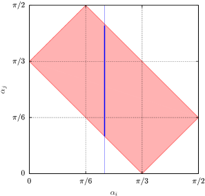
Figure 2.7: Integration limits for the rotation operator eq. (2.44). For a given $\alpha_{i}$ the shaded region determines the interval of integration for $\alpha_{j}$. A specific value of $\alpha_{i}$ is indicated by the thick blue line.

2.2.4 Zero-Range Solution

We now take the zero-range limit, i.e. $U=0$ in eq. (2.41). The solutions with boundary condition $\psi(\pi/2)=0$ are

$$\psi(\alpha_{i})=\mathcal{N}(\rho)\sin(\nu(\alpha_{i}-\frac{\pi}{2})),$$ (2.45)

with normalization $\mathcal{N}(\rho)$ depending on the eigenvalue $\nu(\rho)$. It is straightforward to rotate this solution with eq. (2.44) and we obtain

$${\cal R}[\psi](\alpha_{i})=\mathcal{N}\frac{4}{\sqrt{3}\nu}\left\{\begin{array}[]{ll}\sin(-\nu\alpha_{i})\sin(\nu\frac{\pi}{6})&\text{, }0\leq\alpha_{i}\leq\frac{\pi}{3}\\ \sin(\nu(\alpha_{i}-\frac{\pi}{2}))\sin(\nu\frac{\pi}{3})&\text{, }\frac{\pi}{3}\leq\alpha_{i}\leq\frac{\pi}{2}\;.\end{array}\right.$$ (2.46)

Note that this function is zero at $\alpha_{i}=0$ and $\pi/2$. It is continuous but not differentiable at $\alpha_{i}=\pi/3$, which comes from the fact that the zero-range model has $\psi(0)\neq 0$ (in contrast to any finite-range potential). However, the total wave-function $\Phi$ is smooth everywhere.

We also need to impose a boundary condition at $\alpha_{i}=0$ to determine the eigenvalue $\nu$. In the two-body case the asymptotic radial wave-function is given by $u(r)=rR(r)\propto\sin(kr+\delta(k))$. The zero-range limit can be formulated as the free problem with boundary condition

$$\left.\frac{\partial\ln(rR(r))}{\partial r}\right|_{r=0}=\left.k\cot\delta(k)\right|_{k=0}=-\frac{1}{a}\;.$$ (2.47)

For the three-body problem we apply the same boundary condition in each of the three Jacobi sets (for fixed $\rho$),

$$\left.\frac{\partial\ln(r_{jk}\Phi)}{\partial r_{jk}}\right|_{r_{jk}=0}=-\frac{1}{a}\;.$$ (2.48)

In the limit $r_{jk}\to 0$ we have to lowest order $r_{jk}=\sqrt{2}x_{i}\simeq\sqrt{2}\rho\alpha_{i}$. Using eq. (2.42) the logarithmic derivative then becomes

$$\left.\frac{\partial\ln(r_{jk}\Phi)}{\partial r_{jk}}\right|_{r_{jk}=0}\simeq\left.\frac{1}{\sqrt{2}\rho}\frac{\partial\ln(\psi+2{\cal R}[\psi])}{\partial\alpha_{i}}\right|_{\alpha_{i}=0}$$ (2.49)

to lowest order in $\alpha_{i}$. By inserting eq. (2.45) and eq. (2.46) we obtain

$$\frac{1}{\sqrt{2}\rho}\ \frac{-\nu\cos(\nu\frac{\pi}{2})+\frac{8}{\sqrt{3}}\sin(\nu\frac{\pi}{6})}{\sin(\nu\frac{\pi}{2})}=-\frac{1}{a}\;,$$ (2.50)

which determines the angular eigenvalues $\nu_{n}(\rho)$. This equation was first obtained by V. Efimov [Efi71].

2.2.5 The Efimov Effect, $|a|=\infty$

Let us consider the resonant limit $|a|=\infty$. Then eq. (2.50) has a single imaginary solution $\nu_{0}\simeq 1.00624i$ determined by

$$-\nu\cos(\nu\frac{\pi}{2})+\frac{8}{\sqrt{3}}\sin(\nu\frac{\pi}{6})=0.$$ (2.51)

We will refer to $\nu_{0}$ or the related effective potential $1/\rho^{2}$ as the Efimov solution. The related effective hyper-radial potential becomes

$$V_{\textup{eff},0}(\rho)=-\frac{\hbar^{2}}{2m}\frac{\xi^{2}+1/4}{\rho^{2}},$$ (2.52)

where $\xi=|\nu_{0}|=1.60024$. Since the angular solutions only depend on $\rho$ via the constant eigenvalues $\nu_{n}$, all non-adiabatic couplings $P_{n,n^{\prime}}$, $Q_{n,n^{\prime}}$ vanish and the adiabatic approximation becomes exact in this limit. The lowest hyper-radial equation becomes

$$\left(-\frac{\partial^{2}}{\partial\rho^{2}}-\frac{\xi^{2}+1/4}{\rho^{2}}\right)f_{0}(\rho)=0,$$ (2.53)

where $\kappa=\sqrt{2m(-E)}/\hbar$. Scaling the variables as $\tilde{f}_{0}=f_{0}/\sqrt{\rho}$, $\tilde{\rho}=\kappa\rho$ eq. (2.53) turns into a Bessel equation. The solution is the modified Bessel function of the second kind (of imaginary order) $\tilde{f}_{0}(\tilde{\rho})=K_{i\xi}(\tilde{\rho})$ [AS95, sec. 9.6.1]. Thus the hyper-radial solutions with binding wave number $\kappa^{(n)}$ become

$$f_{0}^{(n)}(\rho)=\sqrt{\rho}K_{i\xi}(\kappa^{(n)}\rho)\simeq\sqrt{\rho}|\Gamma(i\xi)|\sin\left(\xi\ln(\kappa^{(n)}\rho)+\theta\right).$$ (2.54)

The last approximation is for the low-distance limit $\kappa\rho\ll 1$ where we used several identities and expansions for the $\Gamma$ function. The phase $\theta$ is given by $\theta=\textrm{arg}\{\Gamma(-i\xi)2^{-i\xi}\}+\pi/2\simeq 0.874\pi$, and $|\Gamma(i\xi)|\simeq 0.5148$.

We see that the solutions have infinitely many nodes at short distances, meaning that there are infinitely many low-lying states. This is the well known Thomas effect in the three-body problem with zero-range interactions and fixed two-body binding energy (or scattering length $a$) [Tho35, NFJG01].

The Thomas collapse is unphysical since the real short-distance details must be taken into account. Thus, we need to introduce a regularization, e.g. by setting $f_{0}(\rho_{0})=0$ at some short arbitrary distance $\rho_{0}$. Using eq. (2.54) this leads to $\kappa^{(n)}=\exp(-n\pi-\theta)/\rho_{0}$, giving the characteristic scaling between the energies,

$$\frac{\kappa^{(n)}}{\kappa^{(0)}}=e^{-\pi n/\xi}\simeq 22.7^{-n},\quad\textrm{or}\quad\frac{E^{(n)}}{E^{(0)}}=e^{-2\pi n/\xi}\simeq 515.0^{-n}.$$ (2.55)

This is the essence of the Efimov effect, where infinitely many loosely bound states (Efimov trimers) accumulate a zero energy. Three hyper-radial wave-functions are shown in fig. 2.8. The root-mean-square hyper-radii of the Efimov states scale accordingly as

$$\frac{\langle\rho^{2}\rangle_{n}^{1/2}}{\langle\rho^{2}\rangle_{0}^{1/2}}=e^{\pi n/\xi}\simeq 22.7^{n}.$$ (2.56)

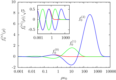
Figure 2.8: Hyper-radial wave-functions, eq. (2.54), for the Efimov states in the effective $1/\rho^{2}$ potential eq. (2.52). The scale $\kappa_{0}$ is the binding wave number for state $n=0$. The solutions have infinitely many nodes as $\rho\to 0$, see inset.

2.2.6 Universal Scaling, $|a|<\infty$

Let us finally discuss the case of finite but large scattering length. The constant solution $\nu_{0}$ in eq. (2.50) still holds, but now only for $\rho\lesssim|a|$, thus the effective $1/\rho^{2}$ potential will be modified at $\rho\gtrsim|a|$. This means that all the Efimov states with hyper-radii larger than $|a|$ (see e.g fig. 2.8) will be affected. However, Efimov states with hyper-radii smaller than $|a|$ only have exponential tails in the affected region and are therefore essentially unchanged. Note also, that the regularization can be considered fixed: The infinite scattering length is tuned by adjusting the two-body energy infinitesimally around zero leaving the underlying finite-range potentials fixed.

The resulting behavior of the Efimov trimer energies, $E_{T}^{(n)}$ , are shown in fig. 2.9 as function of inverse squared scattering length $1/a^{2}$. On the $a>0$ side the two-body system has a shallow bound state (dimer) with energy $E_{D}=-\hbar^{2}/ma^{2}$, eq. (2.8) (indicated by the blue diagonal line). For the three-body case this defines the atom-dimer fragmentation threshold. For $a<0$ the two-body system has a shallow virtual state $E_{V}$ and the three-body system has a three-body fragmentation threshold at zero energy (indicated by the red horizontal line). At $|a|=\infty$ the infinite sequence of Efimov trimers is shown.

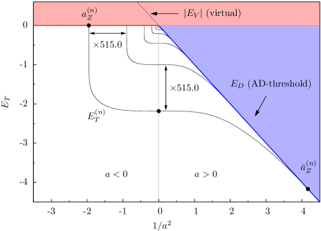
Figure 2.9: Discrete universal scaling of Efimov states. Trimer energy levels, $E^{(n)}_{T}$ are shown as functions of scattering length, $a$. Points indicate the critical scattering lengths where the trimer crosses the trimer and atom-dimer thresholds. Both axes were scaled by a power of ${1/8}$ to reduce the large scaling factor $515.0$ to $2.18$, i.e. the axes actually show $[\hbar^{2}/(ma^{2}E_{\infty})]^{1/8}$ and $[E_{T}/E_{\infty}]^{1/8}$, with $E_{\infty}$ being an arbitrary regularization scale modulo 515.0 (the energy of a trimer at $a=\infty$).

When $a$ is decreased from infinity to $a<0$ the effective hyper-radial potential moves up at large distances $\rho\gtrsim|a|$, and the most loosely bound Efimov trimers are pushed into the continuum. For $a>0$ the effective potential decreases, now converging to the dimer binding energy $V_{\textup{eff}}\to E_{D}<0$ for larger hyper-radii. Each Efimov trimer moves down correspondingly, until it disappear into the atom-dimer continuum.

Because of the scale-invariant $1/\rho^{2}$ potential all the Efimov trimer energies scale the same way, and only a single universal function needs to be calculated. The specific form can be found by solving the Schrödinger or Faddeev equations numerically for short-ranged potentials (as done in chapter 3), or by using effective field theory (EFT) [BH03, BHK03, BH06]. In the exact universal limit the energy $E_{T}^{(n)}$ of the $n$’th trimer state can be parametrized as

$$E_{T}^{(n)}-\frac{\hbar^{2}}{ma^{2}}=e^{\Delta(\varphi)/\xi}e^{-2\pi n/\xi}E_{\infty},$$ (2.57)

where $\xi=1.00624$, $\Delta(\varphi)$ is a universal function [BH06] of the angle $\varphi\in[-\pi;-\pi/4]$ given by $\tan^{2}\varphi=-E_{T}^{(n)}ma^{2}/\hbar^{2}$ (i.e. $\varphi$ is the polar angle in the coordinates of fig. 2.9). $E_{\infty}$ is the regularization scale (here the energy of state $n=0$ at $a=\infty$) which cannot be determined within the zero-range theory. It has to be supplied from phenomenological information.

The two critical scattering lengths $a^{(n)}_{Z}$ and $\bar{a}^{(n)}_{Z}$ where the Efimov trimer $E_{T}^{(n)}$ disappears into the three-body and atom-dimer continuum, see fig. 2.9, are given explicitly in the zero-range limit by [BH06, GME08]

$$a^{(n)}_{Z}=-1.50763/\kappa^{(n)},\quad\bar{a}^{(n)}_{Z}=0.0707645/\kappa^{(n)},$$ (2.58)

where $\kappa^{(n)}=\sqrt{-mE_{T}^{(n)}(a=\infty)}/\hbar$ is the wave number for the $n$’th trimer energy at infinite scattering length.

Three-Body Recombination in Experiments

The critical scattering lengths $a^{(n)}_{Z}$ and $\bar{a}^{(n)}_{Z}$ can be observed via maxima and minima in the atom loss rate of cold gases [KMW⁺06]. In the ultra-cold limit the loss due to two-body collisions $B+B\to B_{2}$ are suppressed by energy-momentum conservation. Therefore three-body collisions $B+B+B\to B+B_{2}$ can be considered as the dominant mechanism for the total loss rate. The general behavior for the three-body recombination rate is $|a|^{4}$ for large $a$ [NM99, EGB99, BH06]. On top of this background additional resonance or interference effects effects from the Efimov trimers should be seen.

The first case where the Efimov trimer disappear into the three-body continuum ($a<0$) leads to a resonant peak in the recombination rate. In numerical hyper-spherical descriptions this is explained by a tunneling into a small $\rho$-region and subsequent decay into strongly bound molecular states [EG06]. The second case where the trimer crosses the atom-dimer threshold ($a>0$) leads to a minima in the recombination rate. This can be explained as two interfering pathways from the incoming hyper-spherical channel to the weakly bound atom-dimer channel [EG06].

Until now, only a few experiments measuring such effect have been performed, namely in ¹³³Cs gases [KMW⁺06, KFM⁺09] and also in a three-component ⁶Li Fermi gas [WLO⁺09]. The experiments will be conclusive when the scaling factor $22.7$ is observed (or a correspondingly smaller factor for unequal mass systems).

2.3 Mean-Field Condensates

The Gross-Pitaevskii (GP) equation is based on a mean-field ansatz with the condensate wave-function (or order parameter) $\Psi(\mbox{\boldmath$r$})$ together with the zero-range contact interaction

$$V_{ZR}(r)=U_{0}\delta(r),\quad U_{0}=\frac{4\pi\hbar^{2}a}{m}.$$ (2.59)

The coupling constant $U_{0}$ is chosen such that the correct energy shift is reproduced, see chapter 7. This is equivalent to a Born approximation where $a_{born}$ is replaced by the physical scattering length $a$. This leads to the GP energy functional

$$E(\Psi)=\int\,\mathrm{d}{\mbox{\boldmath$r$}}\left(\frac{\hbar^{2}}{2m}|\nabla\Psi|^{2}+V_{ext}(\mbox{\boldmath$r$})|\Psi|^{2}+\frac{U_{0}}{2}|\Psi|^{4}\right),$$ (2.60)

which includes kinetic energy, the external trapping potential $V_{ext}$, and the interaction term from eq. (2.59). A variation of this functional with the constraint of fixed particle number $N$ leads to the GP equation

$$\left(-\frac{\hbar^{2}}{2m}\nabla^{2}+V_{ext}(\mbox{\boldmath$r$})+U_{0}|\Psi(\mbox{\boldmath$r$})|-\mu\right)\Psi(\mbox{\boldmath$r$})=0,$$ (2.61)

where $\mu$ is the chemical potential.

The GP equation (or variations and extensions of it) has been able to describe a wide variety of BEC phenomena, e.g. the spatial condensate profile in different traps, solitons in homogeneous condensates, rotating BECs with vortex profiles, stability of low-energy modes etc. [PS02, PS03]. A specific useful approach is the Thomas-Fermi (TF) approximation where the kinetic energy term is neglected and analytical solutions are possible. The approximation holds for repulsive gases ($a>0$) with many particles (e.g. $Na/b_{t}\gg 1$ in the harmonic trap of size $b_{t}=\sqrt{\hbar/(m\omega)}$). See chapter 8 for elaborate discussions.

From the perspective that the contact interaction eq. (2.59) should produce correct energy shifts, it is only the lowest order approximation. In chapter 7 we derive the higher-order interaction term proportional to $\delta(\mbox{\boldmath$r$})\nabla^{2}+\nabla^{2}\delta(\mbox{\boldmath$r$})$, and the related modified GP equation with an extra term. The purpose of chapter 7 is to investigate possible effects of such higher-order terms via variational and numerical solutions. Chapter 7 approaches the same question analytically in the TF limit.

2.4 Stochastic Variational Method

The stochastic variational method (SVM) [SV98, Sor05] is a numerical minimization technique to find approximate solutions of few- and many-body problems. The method is based on two basic ingredients, i) stochastic random sampling and ii) deterministic linear variation.

One of the major advantages of the SVM is that one can calculate a large number of bound states, obtaining both the spectrum and wave-functions directly. Another feature is that one can control the amount of inter-particle correlations allowed in the calculated states – depending on the application one may e.g. look for highly correlated few-body states or weakly correlated many-body states. The method is also numerically efficient and it can be parallelized with close to linear scalability.

2.4.1 The Linear Variational Principle

Let us consider the stationary many-body Schrödinger equation $\hat{H}\Psi=E\Psi$ and denote the eigenfunctions and eigenvalues by $\Psi_{n}$ and $E_{n}$, respectively. The well-known Rayleigh-Ritz variational principle states that the variational energy $\mathcal{E}$ evaluated with an arbitrary trial-function $\Psi$ gives an upper bound to the exact ground state energy of the Hamiltonian $\hat{H}$, i.e.

$$\mathcal{E}=\frac{\langle\Psi|\hat{H}|\Psi\rangle}{\langle\Psi|\Psi\rangle}\geq E_{1}.$$ (2.62)

The approach below extends this principle to any number of excited states.

To find approximate variational solutions to the full Schrödinger equation we first restrict the problem to a smaller space spanned by a (possibly over-complete) set of $K$ basis functions $\psi_{k}$. Let us first express the wave-function in this space, i.e.

$$\Psi=\sum_{k=1}^{K}c_{k}\psi_{k},$$ (2.63)

where $c_{k}$ are expansion coefficients. These coefficients determine $\Psi$ completely within the space $\{\psi_{k}\}$, although the expansion may not be unique. By inserting eq. (2.63) in the Schrödinger equation and projecting onto the $j$’th basis state $\psi_{j}$ we obtain

$$\sum_{k=1}^{K}H_{jk}c_{k}=\mathcal{E}\sum_{k=1}^{K}S_{jk}c_{k}.$$ (2.64)

Here the Hamiltonian matrix elements and the overlap matrix in the basis $\{\psi_{k}\}$ are given by

$$H_{jk}=\langle\psi_{j}|\hat{H}|\psi_{k}\rangle,\quad S_{jk}=\langle\psi_{j}|\psi_{k}\rangle,$$ (2.65)

where the brackets mean integration over all coordinates in $\psi_{k}$. In terms of matrix multiplication, eq. (2.65) reads $\mbox{\boldmath$H$}\mbox{\boldmath$c$}=\mathcal{E}\mbox{\boldmath$S$}\mbox{\boldmath$c$}$, where ${\mbox{\boldmath$c$}}=(c_{1},\dots,c_{K})^{T}$ and $\mbox{\boldmath$H$},\mbox{\boldmath$S$}$ have the matrix elements $H_{jk},S_{jk}$. This is a generalized eigenvalue equation of size $K$ with $K$ real eigenvalues $\mathcal{E}_{1}\leq\dots\leq\mathcal{E}_{K}$ and corresponding eigenfunctions $\mbox{\boldmath$c$}_{1},\dots,\mbox{\boldmath$c$}_{K}$.

The above procedure shows how to find approximate solutions to the full Schrödinger equation within a smaller subspace. Let us now specify what we mean by the term “approximate”. We take the space $\{\psi_{k}\}$ to be fixed, and treat the linear coefficients $c_{k}$ in eq. (2.63) as variational parameters. The variational energy, eq. (2.62), expressed in the basis $\{\psi_{k}\}$ then becomes

$$\mathcal{E}=\frac{\mbox{\boldmath$c$}^{\dagger}\mbox{\boldmath$H$}\mbox{\boldmath$c$}}{\mbox{\boldmath$c$}^{\dagger}\mbox{\boldmath$S$}\mbox{\boldmath$c$}},$$ (2.66)

where $\mbox{\boldmath$c$}^{\dagger}=(c_{1}^{*},\dots,c_{K}^{*})$. The stationary solutions within our subspace correspond to $\partial\mathcal{E}/\partial c_{i}=\partial\mathcal{E}/\partial c_{i}^{*}=0$ for all $i$. We multiply eq. (2.66) by $\mbox{\boldmath$c$}^{\dagger}\mbox{\boldmath$S$}\mbox{\boldmath$c$}$ and take the partial derivative $\partial/\partial c_{i}^{*}$ (with fixed $c_{i}$ and $c_{j},c_{j}^{*}$, $j\neq i$). This leads directly to the generalized eigenvalue equation

$$\mbox{\boldmath$H$}\mbox{\boldmath$c$}=\mathcal{E}\mbox{\boldmath$S$}\mbox{\boldmath$c$}.$$ (2.67)

Thus, the energies $\mathcal{E}$ found by projecting the Schrödinger equation onto the fixed subspace $\{\psi_{k}\}$ are actually the best possible energies as seen from the variational perspective.

Furthermore, it can be shown rigorously [SV98] that the generalized (ordered) eigenvalues $\mathcal{E}_{1}\leq\dots\leq\mathcal{E}_{K}$ are strict upper bounds to the exact (ordered) eigenvalues $E_{1}\leq\dots\leq E_{K}\leq\dots$, namely

$$E_{1}\leq\mathcal{E}_{1},\ \cdots,\ E_{K}\leq\mathcal{E}_{K}.$$ (2.68)

It can also be shown [SV98] that by adding another basis state $\psi_{K+1}$, while keeping the first $\psi_{1},\dots,\psi_{K}$ fixed, the upper bounds in eq. (2.68) can only get better. This linear variational principle extends the Rayleigh-Ritz variational principle to an arbitrary number of bound states.

2.4.2 Basis States and Minimization Procedure

To employ the variational principle above we must generate a set of basis states $\psi_{k}$. These states should form a complete set, or at least be able to describe the physical degrees of freedoms of interest. For the approach to be numerically tractable one should also be able to evaluate the matrix elements $H_{ij}$ and $S_{ij}$ analytically. Common choices [SV98, Sor05] are exponential functions or Gaussians (see below). Each basis state $\psi_{k}$ is then parametrized by one or more nonlinear parameters, which we denote by the single symbol $\alpha^{(k)}$.

There are many different minimization strategies for the SVM. The simplest one is to randomly pick a large number of functions $\phi_{k}$ (i.e. nonlinear parameters $\{\alpha_{k}\}$) and solve (2.67). This approach has two minor disadvantages, i) many of the random basis states $\phi_{k}$ may not be necessary to describe the real eigenstates, and ii) solving the full generalized eigenvalue equation of large dimension is numerically very inefficient. Luckily both issues can be solved by adding or modifying only a single state at a time.

Let us assume that the generalized eigenvalue equation has been solved in the $K$-dimensional space spanned by $\psi_{1},\dots,\psi_{K}$ with resulting eigenvalues $\mathcal{E}_{1},\dots,\mathcal{E}_{K}$ and eigenstates $\phi_{1},\dots,\phi_{K}$. We now expand the space by a single basis state $\psi_{K+1}$. Using the Gram-Schmidt process we construct $\phi_{K+1}$ from $\psi_{K+1}$ which is orthogonal to all other $\phi$’s. In the basis $\phi_{1},\dots,\phi_{K+1}$ the generalized eigenvalue problem (2.67) is almost diagonal and reduces to finding the roots of the simple function

$$D(\mathcal{E}^{\prime})=\sum_{k=1}^{K}\frac{|h_{k}|^{2}}{\mathcal{E}_{k}-\mathcal{E}^{\prime}}-\mathcal{E}^{\prime}-h_{K+1},$$ (2.69)

where $h_{k}=\langle\phi_{k}|\hat{H}|\phi_{K+1}\rangle$. $D(\mathcal{E}^{\prime})$ has exactly $K+1$ roots $\mathcal{E}_{1},\dots,\mathcal{E}_{K+1}$ which are the new eigenvalues. Thus, by adding only a single basis state at a time, the generalized eigenvalue problem reduces to one-dimensional root-finding.

Let us give a short example on how the minimization procedure can be done within the SVM, as shown schematically in fig. 2.10. We start by adding one basis state at a time, minimizing the ground state. For the $k$’th basis state $\psi_{k}$ we stochastically generate a set $\{\beta_{m}\}$ of candidates for the parameters $\{\alpha^{(k)}\}$. For each candidate we solve the generalized eigenvalue equation eq. (2.67) from eq. (2.69). We choose the $\beta_{m}$ giving the lowest ground state $\mathcal{E}_{1}$. All other eigenvalues are also guaranteed to be improved. After all $K$ eigenstates are found one may refine the basis: Redundant basis states can be replaced by new ones still optimizing $\mathcal{E}_{1}$. The entire procedure can then be repeated for excited states.

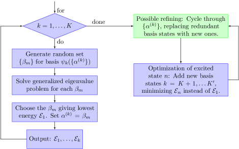
Figure 2.10: A simple example of the SVM minimization procedure. The ground state is found first, followed by a possible refining and minimization of excited states. Since this strategy only changes one basis state at a time, the generalized eigenvalue problem eq. (2.67) reduces to a faster root-finding problem.

This example is quite simple compared to the actual SVM implementation we use [Sor05], but it contains the essential details. The method can be tuned in many ways, e.g. continuous optimization of the random sampling algorithm and selection of appropriate basis states [Sor05].

2.4.3 Center-of-Mass and Symmetrization

The specific many-body Hamiltonian used with the SVM is given by

$$H=-\frac{\hbar^{2}}{2m}\sum_{i=1}^{N}\frac{\partial^{2}}{\partial\mathbf{r}_{i}^{2}}+\frac{m\omega^{2}}{2}\sum_{i=1}^{N}r_{i}^{2}\ +\sum_{i<j}V(\left|\mathbf{r}_{i}-\mathbf{r}_{j}\right|),$$ (2.70)

with a harmonic oscillator trap with angular frequency $\omega$ and trap length $b_{t}=\sqrt{\hbar/(m\omega)}$, and two-body interactions $V(r_{ij})$ chosen either as the zero-range or Gaussian model potentials, eqs. (2.59) and (2.20). Since the confining trap is harmonic, the center-of-mass (cm) $\mbox{\boldmath$R$}=\sum_{i=1}^{N}\mbox{\boldmath$r$}_{i}/N$ can be separated out. We will only consider the center-of-mass ground state motion, i.e.

$$\Psi_{\text{cm}}(\mbox{\boldmath$R$})=\exp(-\frac{NR^{2}}{2b_{t}^{2}}),$$ (2.71)

with corresponding energy $E_{cm}=\frac{3}{2}\hbar\omega$.

Since we consider identical bosons the total wave-function must be completely symmetric with respect to interchange of every pair. This is accomplished with the symmetrization operator

$$\hat{S}=\frac{1}{\sqrt{N!}}\sum_{\sigma}\hat{P}_{\sigma}.$$ (2.72)

Here $\hat{P}_{\sigma}$ is the permutation operator corresponding to the permutation $\sigma$, and the sum is over all possible permutations. The symmetrization does not affect the conclusions of subsection 2.4.1 and 2.4.2 since it is a linear operation. The specific wave-function is then represented as

$$\Psi(\mbox{\boldmath$r$}_{1},\dots,\mbox{\boldmath$r$}_{N})=\Psi_{\text{cm}}(\mbox{\boldmath$R$})\,\hat{S}\sum_{k=1}^{K}c_{k}\,\psi_{k}(\{\alpha_{ij}^{(k)}\},\{\mbox{\boldmath$r$}_{ij}\}).$$ (2.73)

The basis functions, $\psi_{k}$, depend on all the internal coordinates $\{r_{ij}\}$, and are parametrized by a, possibly large, number of variables $\{\alpha_{ij}^{(k)}\}$.

2.4.4 Correlated Gaussians

As the specific basis functions $\psi_{k}$ we use the so-called explicitly correlated Gaussians,

$$\Psi_{\text{full}}=\Psi_{\text{cm}}\,\hat{S}\,\sum_{k=1}^{K}c_{k}\exp\left(-\frac{1}{2}\sum_{i<j}^{N}\alpha_{ij}^{(k)}r_{ij}^{2}\right).$$ (2.74)

This will also be referred to as the full correlated basis. The basis is complete for zero total angular momentum states and it allows all types of clustering in the system. This basis choice allows analytical evaluation of matrix elements for the Gaussian interaction, see [SV98, Sor05]. However, because of the symmetrization the computational complexity is of order $\mathcal{O}(N!)$, and the method is only possible for relatively small number of particles, say $N\lesssim 5$.

The zero-range potential, eq. (2.59), requires an uncorrelated wave-function which we choose in the form of the linear combination of the hyper-radial basis-functions

$$\Psi_{\rho}=\Psi_{\text{cm}}\,\sum_{k=1}^{K}c_{k}\exp\left(-\frac{1}{2}N\alpha^{(k)}\rho^{2}\right),$$ (2.75)

where $\rho$ is the hyper-radius for $N$ particles,

$$\rho^{2}=\frac{1}{N}\sum^{N}_{i<j}r_{ij}^{2}=\sum^{N}_{i=1}(\mbox{\boldmath$r$}_{i}-\mbox{\boldmath$R$})^{2}=\sum^{N}_{i=1}r^{2}_{i}-N\mbox{\boldmath$R$}^{2},$$ (2.76)

generalizing the $N=3$ definition, eq. (2.27). This function is totally symmetric and thus does not require the symmetrization operator ${\hat{S}}$. It is a specific choice for the parameters of eq. (2.74) where the different pairs of particles have the same parameters $\alpha^{(k)}=\alpha_{ij}^{(k)}$, see eq. (2.76). This is reminiscent of a mean-field approximation, since all particles are treated identically. Note that only one basis function $K=1$ with $\alpha^{(1)}=1/Nb_{t}^{2}$ corresponds to the single-particle product of the non-interacting case. The zero-range potential with the hyper-radial variational wave-function eq. (2.75) provides results similar to the Gross-Pitaevskii equation [SFJ05].

For a typical system of trapped atoms even when the scattering length is large the density of the system remains small, $nr_{0}^{3}\ll 1$, and one can assume that only binary collisions play a significant role in the system dynamics. In this approximation the variational wave-function can be simplified by allowing only two-body correlations in the basis-functions,

$$\Psi_{\text{2B}}=\Psi_{\text{cm}}\,\hat{S}\,\sum_{k=1}^{K}c_{k}\exp\left(-\frac{1}{2}N\alpha^{(k)}\rho^{2}-\frac{1}{2}\beta^{(k)}r_{12}^{2}\right),$$ (2.77)

where $\alpha^{(k)}$ and $\beta^{(k)}$ are the nonlinear parameters. This form is equivalent to the Faddeev-Yakubovski expansion $\Psi=F(\rho)\sum_{i<j}\phi(\rho,r_{ij})$ used in [SSJF05a, SSJF05b] where each of the two-body amplitudes only depend on the distance between two-particles. The symmetrization of this function can be done analytically [Sor05, SFJ05] by collecting similar terms which greatly simplifies the numerical calculations. The two-body correlated approach is therefore very useful in dilute many-body systems.

In the trap of size $b_{t}$ with interactions of range $r_{0}$, the non-linear parameters $\alpha_{ij}^{(k)}$ are typically optimized stochastically in an interval from $1/b_{t}^{2}$ to $1/r_{0}^{2}$, or even larger. This allows both short and long-range correlations in the system.

Chapter 3 Efimov Physics: Finite Range and Trap Effects

3.1 Introduction

Much effort has been devoted to extract universal features in many branches of physics, because the applications become more transparent. Several topics concerned with Efimov physics are of special interest here: i) the Efimov effect [Efi70, Efi90] where anomalous three-body properties arise at the threshold of binding of two particles, ii) halos and Borromean systems [JRFG04] where required scaling properties are equivalent to large probabilities in non-classical regions, iii) universality for few-body systems derived from a zero-range interaction [AFT97, FTDA99, BH06], iv) general properties of Bose-Einstein condensates [PS02], and v) their instability due to three-body recombination [KMW⁺06].

In all these five cases the two-body $s$-wave scattering length $a$ is the crucial and only characterizing parameter which is independent of the details of the responsible potentials. In fact the same scattering length can be achieved by disparate potentials. It is highly desirable to assess the uncertainties in the results from the leading order terms and extend to include correction terms. An extension inevitably needs more details which again should be expressed in terms of model-independent parameters. The obvious choice is then to exploit the effective range expansion of the two-body phase shifts where the leading term containing $a$ is given by the zero-energy limit, and the second term is proportional to the energy and the effective range $R_{e}$. Inclusion of even higher-order terms is usually not productive because it is either inefficient or difficult, conceptually and practically.

The purpose of this chapter is to go beyond the scattering length approximation for Efimov physics. We express the corrections in terms of the model-independent, low-energy scattering parameters, scattering length and effective range. For negative scattering lengths an attempt in this direction was made by varying the form of the potentials and computing the critical strengths for few-body binding [RF94, MFK⁺00]. This was aimed at finding the Borromean window where three particles are bound even though all the two-body systems are unbound. The results in [MFK⁺00] are however not expressed in terms of model-independent parameters. Other attempts to include effective range terms within effective field theory are reviewed in [BH06].

Specifically, we calculate the low-lying energy spectrum for three trapped identical bosons interacting via finite-range two-body potentials. The spectrum is compared to results from the zero-range model. The thresholds for trimer binding and atom-dimer binding are extracted and related to effective range corrections. Effective range corrections to Efimov physics and Borromean binding are two aspects of the same effect, and we connect these two regions qualitatively. The Borromean window becomes slightly narrower for substantial effective ranges. The structure at the atom-dimer threshold is an atom far away from the dimer and the major energy correction is due to the change of dimer energy with effective range. This structure becomes less pronounced when the effective range increases. Comparisons with recent results from effective field theory are carried out.

3.2 Procedure

We consider $N=3$ identical bosons with mass $m$ and coordinates $\mbox{\boldmath$r$}_{i}$ in a spherical harmonic trap with frequency $\omega$ and corresponding trap length $b_{t}=\sqrt{\hbar/m\omega}$. As the two-body interaction we mainly use an attractive Gaussian, eq. (2.20), of fixed range $r_{0}$, see fig. 2.3. We also include results for many other potential shapes based on input from [MFK⁺00]. The strength $V_{0}$ is varied within the interval where the potential either cannot support bound states (scattering length $a<0$) or have only one bound state ($a>0$). The positive effective range $R_{e}$ is then also a given function of $V_{0}$. However, near the resonance, $|a|=\infty$, $R_{e}$ varies slowly as function of $V_{0}$. We choose the trap to be much larger than the potential range, $b_{t}/r_{0}=3965$.

The wave functions and energies are found with the stochastic variational method described in chapter 2 using the fully correlated Gaussians, eq. (2.74). The non-linear parameters $[\alpha_{ij}^{(k)}]^{-1/2}$ in eq. (2.74) are optimized stochastically in a large interval covering values of order $r_{0}$ up to values of order $b_{t}$. This allows both short and long-range correlations. The separated center-of-mass motion is given by the lowest oscillator wave function with the energy $E_{cm}=\frac{3}{2}\hbar\omega$.

3.3 Zero-Range Approximation

Let us briefly refresh the results of the zero-range model in chapter 2. In the zero-range limit of the two-body potential, the scattering length $a$ is the only remaining interaction parameter. For $a>0$ the weakly bound dimer has an energy $E_{D}=-\hbar^{2}/(ma^{2})$, eq. (2.8), while the virtual state $E_{V}$ is given by the same expression for $a<0$. The correction to $E_{D}$ and $E_{V}$ in the effective range expansion is given by eq. (2.11). In all numerical applications in this chapter we have found agreement with eq. (2.11) and higher-order terms on the two-body level are not needed.

For three particles many bound Efimov trimers may exist even when the two-body system cannot support any bound states or is weakly bound. The energies $E_{T}^{(n)}$ of these states are given in the zero-range limit by eq. (2.57), see also fig. 2.9. The energies scale geometrically with a factor of 515.0, while the hyper-radii scale with 22.7. The energies are only determined up to a three-body regularization scale, $E_{\infty}\equiv E_{T}^{(0)}(a=\infty)$, which cannot be determined within the zero-range theory. It must be fixed by real finite-range calculations or experimental data.

For $a<0$ the Efimov trimers cross the threshold for three-body binding, while in the opposite direction of $a>0$ the thresholds are crossed for binding of the atom-dimer system. The two corresponding critical scattering lengths $a^{(n)}_{Z}$ and $\bar{a}^{(n)}_{Z}$, corresponding to $E_{T}^{(n)}=0$ and $E_{T}^{(n)}=E_{D}$, are given in the lowest-order zero-range limit by eq. (2.58),

$$a^{(n)}_{Z}=-1.50763/\kappa^{(n)},\quad\bar{a}^{(n)}_{Z}=0.0707645/\kappa^{(n)}.$$ (3.1)

Here $\kappa^{(n)}=(-mE_{T}^{(n)}(a=\infty))^{1/2}/\hbar$ is the wave number for the $n$’th trimer energy at infinite scattering length. The critical scattering lengths $a^{(n)}_{Z}$ ($\bar{a}^{(n)}_{Z}$) can be observed via maxima (minima) in the three-body recombination rate of cold atomic gases [KMW⁺06] as described in chapter 1 and 2. Since, in this lowest order model, the wave number is given by $\kappa=1/a$, eq. (3.1) can instead be written as

$$1/\kappa^{(n)}_{Z}=-1.50763/\kappa^{(n)},\quad 1/\bar{\kappa}^{(n)}_{Z}=0.0707645/\kappa^{(n)},$$ (3.2)

where $\kappa^{(n)}_{Z}$ and $\bar{\kappa}^{(n)}_{Z}$ are the respective critical wave numbers.

3.4 Results

3.4.1 Three-Body Energies: Overview

We compute the energies and wave-functions corresponding to the Hamiltonian in eq. (2.70) with a Gaussian interaction by variation of the form in eq. (2.74). The resulting three-body energies are shown in fig. 3.1 as function of scattering length. The center-of-mass energy is subtracted and the axes have been scaled by a power of $1/8$ in order to obtain a well proportioned figure. The critical scattering lengths and effective ranges for our finite-range calculations are denoted, in analogy to (3.1), with a subscript $F$, i.e. $a^{(n)}_{F}$, $\bar{a}^{(n)}_{F}$, $R^{(n)}_{F}$ and $\bar{R}^{(n)}_{F}$.

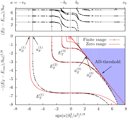
Figure 3.1: Three-body energy levels, $E^{(n)}_{T}$ measured relative to the center-of-mass energy $E_{cm}$, as function of scattering length, $a$. Finite- and zero-range results are shown as points and curves, respectively. As finite-range interaction we use a Gaussian with adjustable depth. The upper and lower parts, corresponding to positive and negative energies, are shown separately. The central value of $|a|=\infty$ corresponds to the threshold for binding two particles. The smallest $a$ (far left and far right) corresponds to the interaction range, $\lvert a\rvert=r_{0}$. There is a quasi-continuum for $a>0$ (shaded) which shows the threshold for atom-dimer binding (individual states are not shown).

The three-body energies obtained in the zero-range model are characterized by the arbitrary regularization scale $E_{\infty}$. We choose it to equal our second trimer energy, i.e. $E_{\infty}=E_{T}^{(2)}(a=\infty)$. The lowest energy, $E_{T}^{(1)}(a=\infty)$, is avoided for regularization because the ground state energy could be influenced by the finite-range properties of the potential whereas the excited spectrum must have the features of the Efimov sequence. However, in fig. 3.1 also the lowest energy coincides with the zero-range result for $|a|=\infty$.

The finite-range calculation only shows three bound trimer states of negative energy in contrast to the infinite series of Efimov states in the free zero-range model. This reflects that the higher lying states are pushed up by the walls of the external field. They now appear in the region of positive energies, still corresponding to bound states, but now determined by the properties of the trap and not the two-body potential.

For $a<0$ the trimer states become less bound and cross the trimer threshold. Deviations from the zero-range model is largest for the lowest state, $n=1$, which is moved to the right in the plot, i.e. towards larger $|a|$. The states $n=2,3$ move in the same direction, but the corrections are much smaller.

For $a>0$ the straight diagonal line shows the atom-dimer zero-range threshold for binding. The corresponding finite-range result is lower and quantitatively in agreement with the dimer energy in eq. (2.11). Only effective range corrections are needed for an accurate description of the dimer energy here. Above the atom-dimer threshold a quasi-continuum is present arising from the dense atom-dimer spectrum confined by the harmonic oscillator potential. The small spacing between these levels is then of order $\hbar\omega$. The three Efimov trimers near the atom-dimer threshold lie below the zero-range result. This is mainly explained by corrections on the dimer energy, as we discuss later.

3.4.2 The $|a|=\infty$ Spectrum

We already commented on the energies at $|a|=\infty$ above, let us now consider the quantitative features. The energies $E_{T}^{(n)}/\hbar\omega$ for $n=1,\dots,7$ are given in the first row of tab. 3.1. The normal Efimov scaling sequence without a trap, is also shown in tab. 3.1. It can of course only describe the lowest bound Efimov states, $n=1,2,3$, and not the trap-like state for $n\geq 4$. Our finite-range results agree well with these zero-range values. The ground state energy, $n=1$, is remarkably close to the zero-range result. The purely attractive Gaussian interaction gives a slightly lower energy, but one could have expected more model-dependence for the ground state. The $n=3$ energy is slightly higher, which is due to the trap, see below. The energy ratios for the finite-range calculations are $(E_{T}^{(n)}-E_{cm})/(E_{T}^{(n+1)}-E_{cm})=530,522$ for $n=1,2$, also in agreement with the zero-range result, $e^{2\pi/s_{0}}=515.0$.

In [JHP02] the energy of three identical bosons in a harmonic trap was considered. Only zero-range interactions and $s$-waves were included. In the limit $|a|/b_{t}=\infty$ the three-body energies, $E_{T}^{(n)}$, are given semi-analytically from the equation

$$\theta=-\textrm{arg}\left\{\frac{\Gamma(\frac{1}{2})-\frac{E_{T}^{(n)}}{2\hbar\omega}-\frac{s_{0}}{2}}{\Gamma(1-s_{0})}\right\},$$ (3.3)

where $s_{0}=1.00624i$ and $\theta$ is a free regularization parameter or three-body phase shift (equivalent to $E_{\infty}$). We fix $\theta=0.404\pi$ to match $E_{T}^{(2)}$ of our finite-range calculations. The resulting spectrum is given in tab. 3.1. All energies agree perfectly with our finite-range results, the deviations being due to numerical errors only (except for the ground state).

	Efimov states			Trap-like states
$n$	1	2	3	4	5	6	7
FR (trap)	$-3.744\cdot 10^{6}$	$-7067$	$-12.04$	$2.78$	$5.10$	$7.05$	$7.47$
ZR (free)$\dagger$	$-3.64\cdot 10^{6}$	$-7067$$\star$	$-13.72$	–	–	–	–
ZR (trap)$\ddagger$	$-3.64\cdot 10^{6}$	$-7067$$\star$	$-12.20$	$2.76$	$5.05$	$6.97$	$7.20$

• Zero-range model in free space, i.e. universal $515.0$ scaling.

• Zero-range model in trap, [JHP02], with $\theta=0.404\pi$ equivalent to $E_{\infty}$.

• This value was used to fix the three-body scale, $E_{\infty}$.

Table 3.1: Efimov trimer energies $E_{T}^{(n)}$ in a trap in units of $\hbar\omega$ for $a=\infty$. The finite-range (FR) calculations are compared with the zero-range (ZR) theory.

3.4.3 Trap-Like States

We already commented on the trap-like states for $|a|=\infty$. Let us now consider the positive energy spectrum for $a<0$ in the upper part of fig. 3.1. This is a “quasi-continuum” with the spacing of order $\hbar\omega$. The asymptotic limit at small $|a|$ is simply the oscillator spectrum for three particles which remains when the two-body interaction is negligibly small. The lowest positive energy level for $a=0$ is $3\times 3\hbar\omega/2$ and the excitation spectrum is obtained by adding $2\hbar\omega$. The almost vertical lines for the Efimov states, continuing into the positive energy region, cross the oscillator states. For small $|a|$ the coupling is also small and the avoided crossing appears like true crossings. As $a$ increases the couplings increase and smooth avoided crossings appear. For $a>0$ a similar spectrum exists, but the huge amount of avoided crossings is not computed.

More generally, the avoided crossings in the upper part of fig. 3.1 resemble the Zel’dovich level rearrangement for two particles, where an attractive long-range potential is perturbed by a strong attractive short-range potential [CKR⁺07]. In our case the long-range interaction is the harmonic trap, and we have three particles instead of two. Also, in [FJT⁺09] we showed how to calculate narrow resonances of three-body systems. The approach was to discretize the continuum by introducing a large artificial oscillator trap. When varying the trap size avoided crossings occurred, and resonance energies and widths could be extracted. Such avoided crossing are closely related to the crossings in fig. 3.1. The only difference is whether the trap or interaction is varied, while the other is fixed.

Recently, Efimov physics in a finite square box with large positive scattering length has been investigated within effective field theory. In the preprint [KH09a] it is concluded that “By decreasing the box size, the binding energy decreases and eventually the state is shifted into the positive energy regime. The finite volume corrections are most important for the shallowest states which are largest in size and feel the finite volume first”. These two conclusions agree with our results above where all but the three lowest Efimov states were pushed up by the harmonic trap. It is also consistent with [JHP02]. The behavior is easily understood from the fact that a confining volume induces extra kinetic (zero-point) energy. However, in the published version [KH09b] the figures were changed and the conclusion was replaced by “If the box size is decreased, the binding increases[ed.]”. This conclusion contradicts all physical intuition and is not elaborated in [KH09b].

3.4.4 Finite-Range Borromean Window Corrections

The differences between finite- and zero-range results for $a<0$ can be extracted from fig. 3.1. We focus on the measurable quantities expressing that an energy threshold has been crossed.

The finite-range results for the negative critical scattering lengths $a^{(n)}_{F}$ are shown in tab. 3.2 for $n=1,2,3$ together with the corresponding effective ranges $R^{(n)}_{F}$. The related zero-range values $a^{(n)}_{F}$ were calculated from eq. (3.1) with the regularization fixed by the finite-range energies $E_{T}^{(n)}-E_{cm}$ from tab. 3.1. The values are shown in fig. 3.2, where we plot the relative shift in critical scattering lengths as functions of effective range. The systematics is discussed below.

	Efimov states
$n$	1	2	3
$a_{F}^{(n)}$	$-4.376$	$-74.09$	$-1631$
$a_{Z}^{(n)}$	$-3.089$	$-71.10$	$-1625$
$R_{F}^{(n)}$	$1.670$	$1.449$	$1.436$

Table 3.2: Critical negative scattering lengths, $a_{F}^{(n)}$, for binding of the $n$’th Efimov trimer state. The finite-range interaction (F) is a Gaussian with range $r_{0}$. The zero-range (Z) results are fixed by the trimers energies at $|a|=\infty$. The effective range at the position for binding is also shown. All values are in units of $r_{0}$.

We note that the first threshold, $a_{F}^{(1)}$, is also significant by marking the interval of scattering lengths where two particles cannot bind while three particles can. This Borromean window between the threshold and $|a|=\infty$, has been calculated in [MFK⁺00] for a number of different radial shapes of the two-body potentials. Their results are expressed as ratios, $S=g_{3}/g_{2}$, of critical strengths required precisely to bind the two and three body systems, respectively. This ratio is limited to $2/3\leq S\leq 1$, but for most ordinary potentials $S\simeq 0.8$. We find $S=0.793$ for the the Gaussian potential in agreement with $0.79$ in [MFK⁺00]. With the critical potential strengths given in [MFK⁺00] we calculate $a^{(1)}_{F}$ and $R^{(1)}_{F}$. The results are compared to the Gaussian values $a^{(n)}_{F}$ and the zero-range results in fig. 3.2. As in fig. 3.1, the effect of the positive effective range is a systematic shift of the critical scattering length towards larger absolute values. The difference decreases with increasing $n$ which implies that most significant effects are related to small $|a|$-values. The available systematics in fig. 3.2 can be described by a straight line, i.e.

$$\frac{a^{(n)}_{F}-a^{(n)}_{Z}}{a^{(n)}_{Z}}=1.3\frac{R^{(n)}_{F}}{|a^{(n)}_{F}|}\;.$$ (3.4)

The wide range of potential shapes used, indicate that this result most probable is model-independent. Although the conclusions are based on calculations with $R_{e}>0$ only, we speculate that eq. (3.4) has the same form for $R_{e}<0$. This implies that the shift of critical scattering length changes sign, i.e. the energies move to the left in fig. 3.1.

The shift in eq. (3.4) should be measurable for cold atomic gases as positions of extrema of the three-body recombination rate near a Feshbach resonance [KMW⁺06]. For broad resonances the background channel (the van der Waals interaction) will determine the effective range. Thus $R_{e}$ will be positive and of the order $l_{vdW}$, and the shift will be toward larger $|a|$. On the other hand, for narrow Feshbach resonances $R_{e}$ is negative and given by eq. (2.14), so the shift will be towards smaller $|a|$.

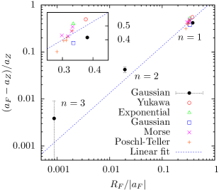
Figure 3.2: The relative shift between finite- and zero-range critical scattering lengths, $a^{(n)}_{F}$ and $a^{(n)}_{Z}$ as function of the corresponding critical effective range $R^{(n)}_{F}$. The Gaussian data from fig. 3.1 are shown with numerical error bars. The other data are for the ground states of different finite-range potentials from [MFK⁺00]. The zero-range energy scale $E_{T}^{(n)}(a=\infty)$ was chosen equal to the individual finite-range energies at $|a|=\infty$. The fit is given in eq. (3.4).

3.4.5 Finite-Range Atom-Dimer Corrections

The effective range corrections are more complicated for $a>0$ because the atom-dimer threshold is also shifted, see fig. 3.1. This effect is investigated in fig. 3.3 (upper part) where the trimer energy is now shown as function of the finite-range dimer energy, $E_{D}$. Then the thresholds coincide for finite- and zero-range models.

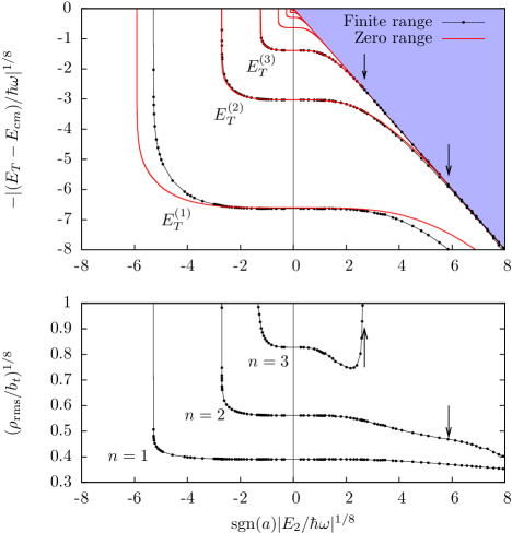
Figure 3.3: Top: Three-body energies, $E^{(n)}_{T}$, as in fig. 3.1, but plotted as function of two-body energy instead of scattering length. On the right part ($a>0$) $E_{2}=E_{D}$ is the weakly bound dimer, eq. (2.11), while on the left part ($a<0$) $E_{2}=E_{V}$ is the shallow virtual dimer (also eq. (2.11)). Bottom: The root-mean-square hyper-radii, $\rho_{\text{rms}}$, as function of two-body energy. The zero-range predictions of the crossing of the Efimov states with the atom-dimer threshold are indicated by arrows.

The ground state size is comparable to the range of the attractive finite-range potential, and hence decreases more strongly with increasing $E_{D}$. As expected this state remains in the discrete region below the atom-dimer threshold. The energies of the excited trimer states $n=2,3$ are in perfect agreement with the zero-range prediction. Only $E_{T}^{(2)}$ is slightly below the zero-range model near the atom-dimer threshold. We conclude that the major shift in trimer energies and threshold scattering lengths are due to effective range corrections to the dimer energy alone.

This is consistent with the explanation in [Efi70, Efi90] that these Efimov states disappear into the atom-dimer continuum. As also described in [BH06] this implies that their structure, as the threshold is approached, converges to the dimer-state with a loosely bound atom at large distance.

This understanding is tested by computing the root-mean-square hyper-radii $\rho_{\text{rms}}=\langle\rho^{2}\rangle^{1/2}$, eq. (2.27), shown in the lower part of fig. 3.3 as function of $E_{D}$. We first consider the $n=3$ state. When $E_{D}$ increases, both the energy and the size of the Efimov state decreases. However, when the state approaches the atom-dimer threshold, the structure changes rather abruptly towards a dimer and a free atom, and hence the radius increases correspondingly fast towards the upper limit, $b_{t}$, defined by the trap. From Fig 3.3, this occurs at ($\bar{a}^{(3)}_{F},\bar{R}^{(3)}_{F})=(84.59,1.423)r_{0}$. This is consistent with the zero-range result $\bar{a}^{(3)}_{Z}=80.9r_{0}$ (indicated by the arrow), since the effective range is small compared to the scattering length. The energy of the $n=2$ Efimov state in fig. 3.3 is also in good agreement with the zero-range result. However, when the state approaches the atom-dimer threshold no drastic increase in size is observed, as for ordinary Efimov states. This can be ascribed to the effective range which is comparable to the scattering length in this regime, namely $(\bar{a}^{(2)}_{F},\bar{R}^{(2)}_{F})=(4.1,1.18)r_{0}$. This effect needs a more careful analysis in the future.

3.4.6 Effective Range Corrections in EFT

After the publication of the above results in [TFJ08c], many of these results have been confirmed qualitatively by effective field theory [PJP09, Pla09]. In this subsection we sum up the common effects and also give quantitative comparisons. In [PJP09] the linear effective range corrections to the three-body energies were calculated for $R_{e}>0$. The main features are presented in their fig. 1, which essentially is identical to fig. 3.3 in this chapter. The following conclusions are given in [PJP09, Pla09]:

1. The three-body spectrum at $|a|=\infty$ is unperturbed when introducing a linear effective range correction.

2. For $a<0$ the critical scattering lengths at the trimer threshold move towards higher $|a|$. The effect is largest for the lowest states.

3. For $a>0$ the effects are in general small (after the dimer energy correction is taken into account). The trimer only becomes slightly more bound.

All these qualitative effects are in perfect agreement with the previous conclusions of this chapter.

Let us now turn to a quantitative comparison of the shift in critical scattering length for $a<0$. Since [PJP09] use the two-body bound state pole (i.e. energy) instead of scattering length, we must repeat the analysis of subsection 3.4.4 using $\kappa^{-1}$ instead of $a$. We include the full effective range corrections in $\kappa$ as given as in eq. (2.10). The result is shown in fig. 3.4.

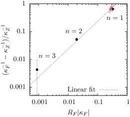
Figure 3.4: Same data as fig. 3.2, but with scattering length $a$ replaced by inverse binding wave number, $\kappa^{-1}$. Legends are the same as in fig. 3.2 and the fit is given in eq. (3.5).

The use of $\kappa^{-1}$, as compared to fig. 3.2, mostly affects the $n=1$ data. The linear relationship becomes marginally better using $\kappa^{-1}$ instead of $a$. The linear fit gives

$$\frac{1/\kappa^{(n)}_{F}-1/\kappa^{(n)}_{Z}}{1/\kappa^{(n)}_{Z}}=2.4R^{(n)}_{F}|\kappa^{(n)}_{F}|.$$ (3.5)

We extract values for the same shift in fig. 1 of [PJP09]. By reading off the critical values for the lowest curve we estimate their lowest order result to be $\kappa_{LO}/\kappa_{0}=-5.68$ and the next-to-lowest order result (including linear $R_{e}$) to be $\kappa_{NLO}/\kappa_{0}=-5.19$. Here $\kappa_{0}$ is an arbitrary momentum scale. The effective range was chosen to be constant, $R_{e}\kappa_{0}=0.01$. This gives

$$\frac{\kappa^{-1}_{NLO}-\kappa^{-1}_{LO}}{\kappa^{-1}_{LO}}/R_{e}|\kappa_{NLO}|=1.8\pm 0.5.$$ (3.6)

This value agrees with the coefficient in eq. (3.5). The difference can be attributed to numerical and read-off errors. Also, the models are based on very different backgrounds and formalisms: In [PJP09] only linear effects in $R_{e}$ are included in an EFT approach, while our finite-range calculations in principle can have minor effects from higher-order shape parameters (i.e. potential model-dependence) and the trap. Taking all these remarks in consideration, the agreement is actually extraordinarily good.

The discussion above is only based on a single value from [PJP09], i.e. the predictions of the linear relationship in eq. (3.5) is not confirmed by EFT yet. Such work is currently in progress, and preliminary results confirm the linear prediction with the correct coefficient.

3.5 Conclusions and Outlook

We have used a basis of correlated Gaussians to calculate the spectrum for three identical bosons for a finite-range potential and an external trap. The scattering length was tuned to arbitrary values, and the many excited states were computed accurately as function of scattering length. The universal spectrum at infinite scattering length was in perfect agreement with analytical models.

We then focused on two thresholds at negative and positive scattering lengths, i.e. the Borromean window where two particles cannot bind while three can form many bound states, and the atom-dimer threshold where dimers can bind and an atom may be bound to the dimer.

We have extracted the universal behavior of both these thresholds, including corrections expressed in terms of effective range divided by scattering length. We also conclude that effective range corrections to Efimov physics and Borromean binding are two aspects of the same effect and these two regions can be connected quantitatively. The linear shift in critical scattering lengths at the trimer threshold agrees quantitatively with effective field theory. The main effect is that the universal scaling factor becomes smaller for the lowest Efimov states (smallest scattering length) on the negative scattering length side.

We also show that the structure as the atom-dimer threshold is approached is a weakly bound atom moving away from the dimer. The main effective range correction to the trimer energies near the atom-dimer threshold then comes from the dimer only. This seems to induce a larger scaling factor for the lowest Efimov states.

The results have observable consequences for three-body recombination rates in atomic Bose-Einstein condensates and should be taken into account when the scattering length is comparable to the effective range [KMW⁺06, KFM⁺09]. The effects are also applicable for halo nuclei and Borromean systems.

Future investigations could repeat a similar analysis with potentials of negative effective range, which could be useful for modeling narrow Feshbach resonances. We speculate that the linear relationship eq. (3.4) also holds for negative effective range. This conjecture is strongly supported in the next chapter, where we analytically derive bounds for the Efimov effect in the case of large negative effective range.

Chapter 4 Conditions for Efimov Physics

4.1 Introduction

We have seen in previous chapters how universal scaling properties in three-body systems arise when the scattering length $a$ is much larger than the range $r_{0}$ of the underlying two-body potential. In this regime several three-body observables are universal. The universal scaling of Efimov trimers is usually said to exist for rms-sizes between $r_{0}$ and $a$ [Efi73, Efi91, BH06, KMW⁺06]. The effective range $R_{e}$ from a low-energy phase shift expansion is sometimes used instead of $r_{0}$ in this statement [FJ01b, TFJ08c, PJP09]. This ambiguity occurs because $r_{0}$ and $R_{e}$ are often of the same order. However, for narrow Feshbach resonances in atomic gases $R_{e}$ can be much larger than $r_{0}$ [BJK05], and the implications for such systems need to be explored.

Zero-range models, in particular in combination with the hyper-spherical approximation [FJ01b, Jon04, BH06], have been successful in semi-quantitative descriptions of three-body systems in the universal regime. Semi-rigorous finite-range corrections have been attempted by including higher-order terms in the effective range expansion [FJ01b, PJP09] as a step towards the full finite-range calculations as in [SEGB02, TFJ08c] while maintaining the conceptual and technical simplicity of the zero-range approximation.

The obvious generalization of the zero-range model, eqs. (2.48)–(2.50), is to substitute $-1/a$ with $-1/a+(R_{e}/2)k^{2}$, where $k$ is the two-body wave number, in the relevant expressions for the logarithmic derivative of the total wave-function at small separation of the particles. However, in three-body systems neither the two-body wave number nor the small separation are uniquely defined, and rigorous inclusion of all terms of the given order is non-trivial. The lack of rigor in previous works could have serious implications for applications where finite-range effects are important, such as the stability conditions for condensates in traps, and in particular for Efimov physics. Experimental progress [KMW⁺06, KFM⁺09] will soon require this increased accuracy near the boundaries of the universal regime.

In this chapter we consider a system of three identical bosons near a Feshbach resonance in the universal regime with large scattering length usually described by model-independent zero-range potentials. We employ the adiabatic hyper-spherical approximation described in chapter 2 and derive the rigorous large-distance equation for the adiabatic potential for finite-range interactions. The equation is suitable for the analytic studies of the finite-range corrections in the three-boson problem. We investigate the finite-range corrections to the adiabatic potential and the non-adiabatic term and compare with the zero-range approximation. The effective range correction to the zero-range approximation must be supplemented by a new term of the same order. The non-adiabatic term can be decisive. Efimov physics is always confined to the range between effective range and scattering length. Our analytical results agree with numerical calculations for realistic potentials.

4.2 Adiabatic Eigenvalue Equation

We first generalize the adiabatic eigenvalue equation, eq. (2.50), to arbitrary finite-range potentials. The derivation is similar to that of chapter 2, but with some modifications.

We consider three identical bosons of mass $m$ and coordinates $\mbox{\boldmath$r$}_{i}$ interacting via a finite-range two-body potential $V$, where we assume $V(r_{jk})=0$ for $r_{jk}=\lvert\mbox{\boldmath$r$}_{j}-\mbox{\boldmath$r$}_{k}\rvert>r_{0}$. Only relative $s$-waves are included. We use the hyper-radius $\rho^{2}=(r_{12}^{2}+r_{13}^{2}+r_{23}^{2})/3$, eq. (2.27) and hyper-angles $\tan\alpha_{i}=(r_{jk}/r_{i,(jk)})\sqrt{3}/2$, where $r_{i,(jk)}=\lvert\mbox{\boldmath$r$}_{i}-(\mbox{\boldmath$r$}_{j}+\mbox{\boldmath$r$}_{k})/2\rvert$. In the following we shall use one set of coordinates and omit the index.

The adiabatic hyper-spherical approximation treats the hyper-radius $\rho$ as a slow adiabatic variable and the hyper-angle $\alpha$ as the fast variable. The eigenvalue $\lambda(\rho)\equiv\nu^{2}(\rho)-4$ of the fast hyper-angular motion for a fixed $\rho$ serves as the adiabatic potential for the slow hyper-radial motion. The eigenvalue is found by solving the Faddeev equations, eq. (2.41), for fixed $\rho$,

$$\Big{[}-\frac{\partial^{2}}{\partial\alpha^{2}}-\nu^{2}+U\Big{]}\psi=-2U{\cal R}[\psi].$$ (4.1)

Here $\psi(\rho,\alpha)$ is the Faddeev hyper-angular component,

$$U(\rho,\alpha)=V(\sqrt{2}\rho\sin\alpha)\frac{2m\rho^{2}}{\hbar^{2}}$$ (4.2)

is the rescaled potential, and

$${\cal R}[\psi](\rho,\alpha)\equiv\frac{2}{\sqrt{3}}\int_{\lvert\frac{\pi}{3}-\alpha\rvert}^{\frac{\pi}{2}-\lvert\frac{\pi}{6}-\alpha\rvert}\psi(\rho,\alpha^{\prime})\,\mathrm{d}\alpha^{\prime}$$ (4.3)

is the operator that rotates a Faddeev component into another Jacobi system and projects it onto $s$-waves, eq. (2.44). The hyper-angular wave-function of the three-body system is

$$\Phi(\rho,\alpha)=\frac{\psi(\rho,\alpha)+2{\cal R}[\psi](\rho,\alpha)}{\sin 2\alpha}.$$ (4.4)

In the adiabatic approximation the hyper-radial function $f(\rho)$ satisfies the ordinary hyper-radial equation, eq. (2.36), with the effective potential

$$V_{\textup{eff}}(\rho)=\frac{\hbar^{2}}{2m}\left(\frac{\nu^{2}-1/4}{\rho^{2}}-Q\right),\quad\,Q=\left\langle\Phi\right|\frac{\partial^{2}}{\partial\rho^{2}}\left|\Phi\right\rangle,$$ (4.5)

where $Q$ is the non-adiabatic term and $\Phi$ is normalized to unity for fixed $\rho$.

We first divide the $\alpha$-interval $[0;\pi/2]$ into two regions: (I) where $U\neq 0$, and (II) where $U=0$. The regions are separated at $\alpha=\alpha_{0}$ where $\sin\alpha_{0}\equiv r_{0}/(\sqrt{2}\rho)$.

Region (II): Here $U=0$ and we have the free solution to eq. (4.1),

$$\psi^{II}(\alpha)=\mathcal{N}(\rho)\sin(\nu(\alpha-\frac{\pi}{2})),$$ (4.6)

with the boundary condition $\psi^{II}(\pi/2)=0$ and normalization $\mathcal{N}(\rho)$.

Region (I): We now restrict the problem to be outside the “collapsed” region defined by $\rho\geq\rho_{c}\equiv\sqrt{2}r_{0}$. This implies that $\alpha_{0}\leq\pi/6$. Since $\alpha\leq\alpha_{0}$ the rotation operator, eq. (4.3), only integrates over the free solution $\psi^{II}$, see fig. 4.1.

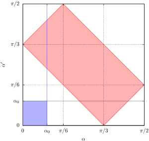
Figure 4.1: Integration limits for the rotation operator eq. (4.3). For $\rho>\rho_{c}$ the shaded regions does not overlap and the three-body problem reduces to an effective two-body problem. When $\alpha\leq\alpha_{0}\leq\pi/6$ the integration limit for $\alpha^{\prime}$ is strictly outside the potential range $[0:\alpha_{0}]$ giving ${\cal R}[\psi]={\cal R}[\psi^{II}]$.

Equation (4.1) then simplifies to

$$\Big{[}-\frac{\partial^{2}}{\partial\alpha^{2}}-\nu^{2}+U\Big{]}\psi^{I}=-2U{\cal R}[\psi^{II}].$$ (4.7)

The solution is $\psi^{I}=\psi^{Ih}-2{\cal R}[\psi^{II}]$, where $\psi^{Ih}$ and $-2{\cal R}[\psi^{II}]$ are homogeneous and inhomogeneous solutions, respectively. $\psi^{Ih}$ is the regular solution to

$$\Big{[}-\frac{\hbar^{2}}{m}\frac{\partial^{2}}{\partial r^{2}}-\frac{\hbar^{2}k_{\rho}^{2}}{m}+V_{\rho}(r)\Big{]}\psi^{Ih}=0,$$ (4.8)

$$V_{\rho}(r)\equiv V(\sqrt{2}\rho\sin(\frac{r}{\sqrt{2}\rho})),$$ (4.9)

where $k_{\rho}=\nu/(\sqrt{2}\rho)$ and $r=\sqrt{2}\alpha\rho$. When $\alpha\to\alpha_{0}$,

$$\psi^{Ih}\propto\sin(k_{\rho}r+\delta_{\rho}),$$ (4.10)

where the modified phase shift $\delta_{\rho}(k_{\rho})$ arises from the modified two-body potential, $V_{\rho}$.

The solutions $\Phi$ in region (I) and (II) are now matched smoothly, giving

$$\left.\frac{\partial}{\partial\alpha}\ln\psi^{Ih}\right|_{\alpha_{0}}=\left.\frac{\partial}{\partial\alpha}\ln\left(\psi^{II}+2{\cal R}[\psi^{II}]\right)\right|_{\alpha_{0}}.$$ (4.11)

After inserting eqs. (4.6) and (4.10), this equation becomes

$$\frac{1}{\sqrt{2}\rho}\ \frac{-\nu\cos(\nu\frac{\pi}{2})+\frac{8}{\sqrt{3}}\sin(\nu\frac{\pi}{6})}{\sin(\nu\frac{\pi}{2})}=k_{\rho}\cot\delta_{\rho}(k_{\rho}),$$ (4.12)

which defines $\nu$ as function of $\rho$. This generalizes the $-1/a$ expression for the lowest-order zero-range model, eq. (2.50).

The right-hand-side deviates from the zero-range approximations [Jon04, PJP09] which use the normal two-body phase shift, i.e. the right-hand-side is $k_{\rho}\cot\delta(k_{\rho})$. We use the rigorously defined phase shift $\delta_{\rho}$ for $V_{\rho}$ instead of $\delta$. Our result is exact for $\rho\geq\rho_{c}$.

4.3 Effective Range Expansion

In the limit $\rho\gg\rho_{c}$, the $\rho$-dependent potential, $V_{\rho}(r)$, approaches $V(r)$, and consequently $\delta_{\rho}$ approaches $\delta$. The $\rho$-dependent low-energy effective range expansion corresponding to $V_{\rho}$ is then to second order

$$k_{\rho}\cot\delta_{\rho}(k_{\rho})\Big{|}_{k_{\rho}\to 0}\approx-\frac{1}{a(\rho)}+\frac{R_{e}(\rho)}{2}k_{\rho}^{2},$$ (4.13)

where $a(\rho)$ and $R_{e}(\rho)$ are functions of $1/\rho^{2}$ that converge to $a$ and $R_{e}$ for $\rho\to\infty$. Up to $1/\rho^{2}$ in eq. (4.13) we get

$$\frac{1}{a(\rho)}\approx\frac{1}{a}+R_{V}\frac{1}{2\rho^{2}},\quad R_{e}(\rho)\approx R_{e}.$$ (4.14)

The model-dependent expansion parameter $R_{V}$, which we shall call the “scattering length correction”, is found to be

$$R_{V}=\frac{m}{6\hbar^{2}}\langle V^{\prime}r^{3}\rangle_{u}=\frac{m}{6\hbar^{2}}\int_{0}^{r_{0}}V^{\prime}(r)r^{3}u(r)^{2}\,\mathrm{d}r,$$ (4.15)

where $u$ is the zero-energy two-body radial wave-function, asymptotically equal to $1-r/a$. Equation (4.12) then becomes

$$\frac{1}{\sqrt{2}\rho}\ \frac{-\nu\cos(\nu\frac{\pi}{2})+\frac{8}{\sqrt{3}}\sin(\nu\frac{\pi}{6})}{\sin(\nu\frac{\pi}{2})}=-\frac{1}{a}+\frac{R_{e}}{2}\ \frac{\nu^{2}}{2\rho^{2}}-\frac{R_{V}}{2\rho^{2}}.$$ (4.16)

This equation without the last two finite-range terms has the well-known purely imaginary solution $\nu_{0}=1.00624i$, or $\lambda_{0}=-5.0125$, for $\sqrt{2}\rho\ll\lvert a\rvert$. This solution gives $V_{\textup{eff}}\propto-1/\rho^{2}$ which is the basis of Efimov physics. The $R_{e}$-term was included in [FJ01b, PJP09], but not the model-dependent $R_{V}$-term. The latter term makes the finite-range corrections to the zero-range adiabatic eigenvalues explicitly non-universal. The last two terms in eq. (4.16) restrict the solution $\lambda_{0}$ to the region $\lvert R_{0}\rvert\ll\sqrt{2}\rho\ll\lvert a\rvert$, where

$$R_{0}\equiv\frac{R_{e}}{2}\nu_{0}^{2}-R_{V},$$ (4.17)

as seen in fig. 4.2 where the lowest solution to eq. (4.16) is shown for different parameter choices. Thus, naively one would think that the lower limit for Efimov physics is determined by the model-dependent length $\lvert R_{0}\rvert$. However, we will show later that $Q$ restores universality and recovers the model-independent effective range, $R_{e}$.

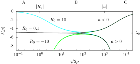
Figure 4.2: Adiabatic eigenvalues $\lambda(\rho)$ from eq. (4.16) as function of hyper-radius $\rho$, for large scattering length $a$ and negative $R_{e}$. Different values of the model-dependent length $R_{0}$ are used, showing that the universal solution $\lambda_{0}$ exists in the region $\lvert R_{0}\rvert\ll\sqrt{2}\rho\ll\lvert a\rvert$. Lengths are in units of $\lvert R_{e}\rvert$.

First, to illustrate the necessity of both $1/\rho^{2}$-terms in eq. (4.16) we consider a large negative effective range corresponding to a narrow Feshbach resonance [BJK05]. To model the large $\lvert R_{e}\rvert$ we pick the attractive potential with barrier, eq. (2.23),

$$V(r)=D\ \text{sech}^{2}\left(\chi\frac{r}{r_{0}}\right)+B\exp\left(-2(\chi\frac{r}{r_{0}}-2)^{2}\right),$$ (4.18)

where $D=-138.27$, $B=128.49$ in units of $\hbar^{2}/(mr_{0}^{2})$, and $\chi=4.6667$. The potential is negligible outside the range $r_{0}$. The low-energy parameters are $a=556.88$, $R_{e}=-142.86$, $R_{V}=73.031$, and $R_{0}=-0.71$ in units of $r_{0}$. In fig. 4.3 we compare $\lambda(\rho)$ obtained by exact numerical solution of the Schrödinger equation [SEGB02] containing the interaction eq. (4.18) with the solution of eq. (4.16). In the zero-range model (including only $1/a$), the $-\rho^{2}$ divergence for large $\rho$ is below the numerical solution. At small distances, $\lambda$ approaches $\lambda_{0}$, above the numerical solution. Inclusion of the $R_{e}$-term, as in [FJ01b, PJP09], provides a better large-distance behavior (since the dimer binding energy is corrected), but overshoots dramatically for $\sqrt{2}\rho\lesssim a$ by approaching $\lambda=-4$. Including consistently both $R_{e}$- and $R_{V}$-terms leads to complete numerical agreement with the exact numerical solution except for very small $\rho$-values near $\rho_{c}$ where higher-order terms are needed in eq. (4.16).

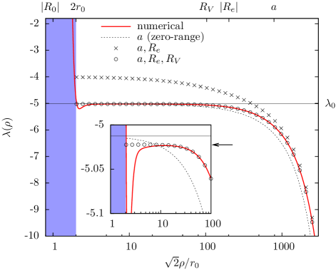
Figure 4.3: Exact numerical adiabatic eigenvalues $\lambda(\rho)$ for a potential with barrier, eq. (4.18) (solid red line), compared to solutions of the eigenvalue equation, eq. (4.16). The zero-range model (dotted line) includes only $a$. Crosses include $a,R_{e}$-terms and circles include $a,R_{e},R_{V}$-terms. The inset shows details around $\lambda_{0}$. The arrow indicates the effect of the correction $\lambda_{0}-2R_{0}/R_{e}$. The shaded region is $\rho<\rho_{c}$.

4.4 Non-Adiabatic Corrections

We now show that the non-adiabatic term restores model-independence and recovers $\lvert R_{e}\rvert$ as the limit for the region of Efimov physics. For simplicity we only consider the limit $\lvert a\rvert=\infty$ and assume $\lvert R_{0}\rvert\ll\lvert R_{e}\rvert$. We first consider $\sqrt{2}\rho\ll\lvert R_{e}\rvert$ (region A in fig. 4.2). Expansion of eq. (4.16) to first order in $(\nu-\nu_{0})$ gives a small constant correction

$$\nu=\nu_{0}-\frac{R_{0}}{\nu_{0}R_{e}}\left(1+O(\frac{\rho}{R_{e}})\right).$$ (4.19)

This correction is marked by the arrow in fig. 4.3 (it is out of the range of fig. 4.2). This gives

$$V_{\textup{eff}}(\rho)=\frac{\hbar^{2}}{2m}\left(\frac{\nu_{0}^{2}-1/4-2R_{0}/R_{e}}{\rho^{2}}-Q\right).$$ (4.20)

To evaluate $Q$ we note that a large negative effective range (for $\lvert a\rvert=\infty$) implies that the two-body wave-function $u$ is localized mainly inside the potential range, as discussed in chapter 2. Then the angular three-body wave-function $\Phi$ can be approximated by $u/\sin(2\alpha)$, i.e. $\psi\simeq u$ and neglecting rotated terms ${\cal R}[\psi]$. The result is $Q=c/\rho^{2}$, where $c\simeq-5/4$ as confirmed numerically. This term cancels the main $1/\rho^{2}$-part in eq. (4.20) and hence prohibits Efimov physics for $\sqrt{2}\rho\ll\lvert R_{e}\rvert$. The intuitive reason is that the two-body wave-function is essentially zero outside the potential, despite the large scattering length, and hence three particles can not interact at large distances.

When $\sqrt{2}\rho\gg\lvert R_{e}\rvert$ (region B in fig. 4.2) we find

$$\nu=\nu_{0}+\nu_{0}c_{0}\frac{R_{0}}{\sqrt{2}\rho}\left(1+O(\frac{R_{e}}{\rho})\right),$$ (4.21)

where

$$c_{0}=\frac{\sin(\nu_{0}\frac{\pi}{2})/\nu_{0}}{\frac{4\pi}{3\sqrt{3}}\cos(\nu_{0}\frac{\pi}{6})-\cos(\nu_{0}\frac{\pi}{2})+\nu_{0}\frac{\pi}{2}\sin(\nu_{0}\frac{\pi}{2})}\simeq-0.671.$$ (4.22)

This gives the effective hyper-radial potential

$$V_{\textup{eff}}(\rho)=\frac{\hbar^{2}}{2m}\left(\frac{\nu_{0}^{2}-1/4}{\rho^{2}}+\frac{c_{0}\nu_{0}^{2}}{\sqrt{2}\rho^{3}}\left(R_{e}\nu_{0}^{2}-2R_{V}\right)-Q\right).$$ (4.23)

The $1/\rho^{3}$ dependence of the correction to the Efimov potential $1/\rho^{2}$ was expected [Efi91]. The model-independent term proportional to $R_{e}/\rho^{3}$ was recently calculated in [PJP09]. However, we also get a model-dependent term $R_{V}/\rho^{3}$ which is of the same order. $Q$ generally receives contributions both from distances inside and outside the finite-range potential. Zero-range models only have the external part of the wave-function, which depends on $\rho$ only though the eigenvalue $\nu(\rho)$. The zero-range result for $Q$ is then

$$Q_{\textup{ZR}}=M_{0}(\frac{\partial\nu}{\partial\rho})^{2}=M_{0}c_{0}^{2}\nu_{0}^{2}\frac{R_{0}^{2}}{2\rho^{4}},$$ (4.24)

where $M_{0}=\langle\Phi|\partial^{2}\Phi/\partial\nu^{2}\rangle|_{\nu=\nu_{0}}$. This fourth order correction can be neglected in eq. (4.23), as was done in [PJP09]. However, the internal part of the wave-function contributes to order $1/\rho^{3}$. To estimate this $1/\rho^{3}$-term we take the analytically solvable finite square well potential of range $r_{0}$ and $\lvert a\rvert=\infty$. This fixes $R_{e}=r_{0}$ and $R_{V}=n^{2}\pi^{2}r_{0}/24$ where $n$ is the number of bound states (including the zero-energy state). We find

$$Q_{\textup{box}}=c_{0}\nu_{0}^{2}(\frac{R_{e}}{2}-2R_{V})\frac{1}{\sqrt{2}\rho^{3}},$$ (4.25)

neglecting $1/\rho^{4}$-terms. The model-dependent $R_{V}$-terms in eqs. (4.23) and (4.25) cancel exactly, giving

$$V_{\textup{eff}}^{\textup{box}}(\rho)=\frac{\hbar^{2}}{2m}\left(\frac{\nu_{0}^{2}-1/4}{\rho^{2}}+c_{0}\nu_{0}^{2}(\nu_{0}^{2}-\frac{1}{2})\frac{R_{e}}{\sqrt{2}\rho^{3}}\right).$$ (4.26)

So the effective potential receives a $R_{e}/\rho^{3}$ correction where the model-dependent coefficient is different from zero-range models [PJP09] because of the inclusion of $Q$. We also expect the $R_{V}$-terms to cancel for general potentials. In conclusion, the Efimov effect persists for $\sqrt{2}\rho\gg\lvert R_{e}\rvert$.

4.5 Atom-Dimer Potential

We have seen that model-dependent corrections to $\lambda_{0}$ are cancelled by equivalent terms in $Q$. A similar effect occurs for the atom-dimer channel potential. Suppose the binding energy is $B_{D}=\hbar^{2}k_{D}^{2}/m$ with corresponding wave number $k_{D}>0$. Then $\nu=ik_{D}\sqrt{2}\rho$ is an asymptotic solution to eq. (4.12) and $\lambda$ diverges as $-\rho^{2}$ corresponding to a bound dimer and a free particle. For this solution, the effective range expansion eq. (4.13) does not hold, since asymptotically $k_{\rho}\to ik_{D}$ is finite. Instead eq. (4.8) reduces to the radial two-body equation, with a normalized bound state $s$-wave function $u_{D}(r)$. Treating $V_{\rho}-V\propto 1/\rho^{2}$ as a perturbation gives the correction

$$\frac{\lambda+4}{2\rho^{2}}=-k_{D}^{2}-\frac{1}{2}\int_{0}^{\infty}\!\!\!r^{3}u_{D}^{2}\frac{mV^{\prime}(r)}{6\hbar^{2}}\,\mathrm{d}r\frac{1}{\rho^{2}}+O(\frac{1}{\rho^{4}}).$$ (4.27)

Since ${\cal R}[\psi]$ is exponentially small for the atom-dimer solution, $Q$ can be computed using the unperturbed wave-function $\psi=\sqrt{\rho}u_{D}(\sqrt{2}\alpha\rho)$, giving

$$Q=-\frac{1}{4\rho^{2}}+\int_{0}^{\infty}\!\!u_{D}(ru_{D}^{\prime}+r^{2}u_{D}^{\prime\prime})\,\mathrm{d}r\frac{1}{\rho^{2}}+O(\frac{1}{\rho^{4}}).$$ (4.28)

The term $-1/(4\rho^{2})$ for the atom-dimer solution is well-known and sometimes referred to as the Langer correction [NM99].

By using the two-body radial equation and partial integration the two integrals in eqs. (4.27) and (4.28) cancel. Thus the $1/\rho^{2}$-terms in the effective potential eq. (4.5) cancel exactly, giving $V_{\textup{eff}}(\rho)=-B_{D}$ up to order $1/\rho^{4}$. Thus $V_{\textup{eff}}$ only depends on $R_{e}$ through $B_{D}$.

4.6 Applications near Feshbach Resonances

The effective range near a narrow Feshbach resonance can be estimated as in eq. (2.14). As an example with a noticeable effect we take the alkali atoms ³⁹K with the very narrow Feshbach resonance at $B=825$G having parameters $\Delta B=-32$mG, $\Delta\mu=-3.92\mu_{B}$, and $a_{bg}=-36a_{0}$ [DZF⁺07]. This gives the large effective range $R_{e}=-2.93\times 10^{4}a_{0}$. For ³⁹K, $r_{0}$ is of the order of the van der Waals length $l_{\textup{vdW}}=1.29\times 10^{2}a_{0}$ [BH06]. Since $\lvert R_{e}\rvert\gg r_{0}$, $\lvert R_{e}\rvert$ determines the lower limit for Efimov physics and corrections to the universal regime are of order $R_{e}/a$ (not $l_{\textup{vdW}}/a$). Thus, the window for universal physics is reduced.

Another example is the Feshbach resonance at $B_{0}=-11.7$G ($\Delta B=28.7$G, $a_{bg}=2.30a_{0}$, $\Delta\mu=2.3\mu_{B}$ [CGJT09]) in ¹³³Cs where [KMW⁺06] apparently have observed a single Efimov state. In this case the effective range estimated from the Feshbach model, eq. (2.14), is $R_{e}=-0.34a_{0}$. This is much smaller than $l_{vdW}=202.0a_{0}$ [CGJT09], thus $l_{vdW}$ is the dominating scale for effective range corrections. The linear effective range corrections of chapter 3 could be applied here.

4.7 Conclusions and Outlook

We have considered a three-body system of identical bosons with large scattering length modeling a Feshbach resonance. The Efimov physics occurring in this universal regime is customarily accounted for by zero-range models. We used the adiabatic hyper-spherical approximation and derived rigorously a transcendental equation to determine the adiabatic potential for a general finite-range potential. We have solved this equation for large scattering length, investigated finite-range effects, and compared with exact numerical results.

Inclusion of the effective range correction to the adiabatic potential is insufficient in general. Crucial corrections of the same order must also be included from both a “scattering length correction” ($R_{V}$) and the non-adiabatic term. These two contributions may separately be large but they tend to cancel each other. Accurate results in zero-range models must account for these new corrections. In conclusion, for large negative effective range the window for Efimov physics is precisely open between the effective range (not the potential range) and the scattering length.

Chapter 5 $N$-Body Efimov Effect

5.1 Introduction

The Efimov effect appears in quantum three-body systems when attractive interactions between at least two pairs of particles are such that the scattering length is much larger than the range of the interaction; in other words two of the three two-body subsystems are close to the threshold of binding. Under these conditions a characteristic series of weakly bound and spatially extended Efimov states appears in the system. These states appear due to specific long-range two-body correlations between particles caused by the large scattering length. The effect is easiest to see in the hyper-spherical adiabatic approximation, chapter 2, where the slow adiabatic variable is the hyper-radius $\rho$. It has been shown [FJ93] that close to the two-body threshold the effective adiabatic potential $V_{\textup{eff}}(\rho)$ is attractive and asymptotically proportional to the inverse square of the hyper-radius,

$$V_{\textup{eff}}(\rho)=-\frac{\hbar^{2}}{2m}\frac{\xi^{2}+1/4}{\rho^{2}},$$ (5.1)

where $m$ is the atomic mass, and $\xi$ is a constant depending on masses of the particles [NFJG01, NFJ98]. For three identical bosons this constant is given by $\xi_{3}=1.00624$ leading to the scaling factors

$$S_{3}=\exp(\pi/\xi_{3})\simeq 22.7\quad\text{and}\quad S_{3}^{2}\simeq 515.0,$$ (5.2)

for radii and energies, respectively. This is equivalent to a geometric series of bound states with exceedingly small energies, $E_{n}\propto e^{-2\pi n/\xi_{3}}$, and exceedingly large root-mean-square hyper-radii, $\langle\rho^{2}\rangle_{n}^{1/2}\propto e^{\pi n/\xi_{3}}$, where $n$ is the state number.

It was shown by Amado and Greenwood that in an $N$-body system with $N>3$ the Efimov effect does not exist at the $N-1$ threshold [AG73]. In particular, for $N=4$ there is no infinite sequence of four-body states at the trimer threshold. This does not rule out an $N$-body Efimov effect at the two-body threshold where the scattering length $a$ is infinite. Of course, weakly bound $N$-body states at $a=\infty$ can not be true bound states, since at this point the clusters with three and higher number of particles are generally deeply bound. The states would then be unstable due to lower lying thresholds and would decay into deeply bound cluster states.

However it has been suggested in [SFJ02] that a sequence of meta-stable $N$-body states with the characteristic exponential energy dependence can yet show up at the two-body threshold. Using the $N$-body hyper-spherical method it has been shown that an $N$-body system at the two-body threshold has a hyper-spherical adiabatic potential with inverse-square dependence. This peculiar adiabatic potential appears due to the same mechanism as for three particles and thus gives rise to $N$-body Efimov states with a structure similar to that of three-body Efimov states: An (otherwise) uncorrelated system with very specific two-body correlations caused by the large scattering lengths.

This specific hyper-spherical adiabatic potential is not the lowest one as different bound clusters with lower thresholds create lower lying adiabatic potentials. However, although not truly bound, these $N$-body Efimov states might still exist as meta-stable states slowly decaying into clusters, much like the Bose-Einstein condensate states. The structure of the Efimov states is determined by the long-range two-body correlations and is thus quite dissimilar to the structure of clusterized states with short-range many-body correlations. Therefore the overlap between Efimov states and clusterized states should be small and consequently the life-time should be large.

The conclusions about meta-stable $N$-body Efimov states were obtained in [SFJ02] in an hyper-spherical adiabatic approximation where the couplings to all other channels were neglected. In this chapter we report on a more realistic calculation of $N$-body Efimov states with a different method, namely the two-body correlated Gaussian stochastic variational method where no adiabatic approximation is assumed. We calculate spectra of trapped systems of $N=3,4,5,6$, and 7 bosons: For each system the calculations reveal a series of Efimov states where the energies and the radii exhibit the characteristic exponential dependence upon the state number. We obtain the new scaling factors for $N>3$ and compare with analytical results from the hyper-spherical adiabatic approach. Finally, we discuss observable consequences.

5.2 Numerical Results

5.2.1 The System and Procedure

We consider a system of $N$ identical bosons with mass $m$ and coordinates $\mathbf{r}_{i}$ in a spherical harmonic trap with frequency $\omega$ and trap length $b_{t}=\sqrt{\hbar/(m\omega)}$. The two-body potential is an attractive Gaussian, eq. (2.20), with range $r_{0}$ and depth $V_{0}$. As in chapter 3 we choose the trap to be much larger than the potential range, $b_{t}/r_{0}=3965$. The depth is tuned around $V_{0}\simeq-2.68\hbar^{2}/(mr_{0}^{2})$ where the first bound state is at the threshold, giving $|a|\gg b_{t}$.

The Schrödinger equation for the Hamiltonian in eq. (2.70) is solved numerically with the stochastic variational method of chapter 2, using the two-body correlated basis, eq. (2.77). The non-linear parameters in the wave-function are optimized stochastically by random sampling in a region that covers the spatial distances from $r_{0}$ to $b_{t}$, which allows us to describe states over many length scales and energies.

We look for $N$-body Efimov states with the structure analogous to that of the three-body Efimov states. The spatial extension of such state should be much larger than the range of the potential $r_{0}$ and smaller than the trap length $b_{t}$.

5.2.2 Universal Energies and Radii

The energies of Efimov states in a trap should be on one hand much larger than the typical energy scale of a cluster state, ${\hbar^{2}/(mr_{0}^{2})}$, and on the other hand smaller than the oscillator energy $\hbar\omega={\hbar^{2}/(mb_{t}^{2})}$. We have calculated the spectrum for $N=3,4,5,6$, and 7 bosons. The calculated energies are shown in fig. 5.1. Indeed, in the indicated energy region each of the $N$-body systems have a series of states with exponential dependence upon the state number, $E_{n}\propto e^{-2\pi n/\xi_{N}}$. The exponential fits give the scaling constants $S_{N}=\exp{\pi/\xi_{N}}$, namely $S_{3}=23.6(4)$, $S_{4}=5.47(40)$, $S_{5}=2.45(4)$, $S_{6}=1.93(2)$, and $S_{7}=1.66(1)$. The indicated statistical errors are from the fits, while the uncertainty related to numerical convergence is not included. This is expected to be largest for $N=3,4$ which use only a few states for the fit. The $N=3$ result agrees with the known analytical result of 22.694 [BH06].

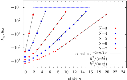
Figure 5.1: Energy $E_{n}$ as function of the state number $n$ for negative energy states of a system of $N$ bosons in a harmonic trap with length $b_{t}$ interacting via an attractive potential of range $r_{0}$ with scattering length much larger than $b_{t}$. The horizontal lines demarcate the region where the Efimov states can exist in trapped gases. The lines show the exponential fits of the form $E_{n}\propto e^{-2\pi n/\xi_{N}}$ drawn through the points in the indicated region.

The spatial extension of Efimov states in trapped systems must also be much larger than the interaction range $r_{0}$ and much smaller than the trap length $b_{t}$. The average size of the state can be described with the ($N$-body) hyper-radius $\rho$,

$$\rho^{2}=\frac{1}{N}\sum^{N}_{i<j}r_{ij}^{2}=\sum^{N}_{i=1}(\mbox{\boldmath$r$}_{i}-\mbox{\boldmath$R$})^{2}=\sum^{N}_{i=1}r^{2}_{i}-N\mbox{\boldmath$R$}^{2},$$ (5.3)

where $r_{ij}$ is the pair distance and $R$ the center-of-mass. On fig. 5.2 are shown the calculated r.m.s. hyper-radii $\langle\rho^{2}\rangle_{n}^{1/2}$ as function of state number $n$. The radii of the Efimov states identified on fig. 5.1 are reproduced well with the exponentials $\langle\rho^{2}\rangle_{n}^{1/2}\propto e^{\pi n/\xi_{N}}$ where the parameters $\xi_{N}$ are taken from the fits on fig. 5.1. Apparently all these states fall within the correct boundaries and the values of the radii follow the correct exponential trend.

There are a few states in the $N=6$ and 7 systems with radii much smaller than those of the typical states in the series with similar energies, see fig. 5.2. Clearly these states are not Efimov states but rather relatively compact states with a different structure. We believe that these states are caused by missing convergence or numerical inaccuracies.

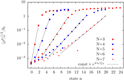
Figure 5.2: Root-mean-square hyper-radius $\langle\rho^{2}\rangle_{n}^{1/2}$ as function of the state number $n$ of a system of $N$ bosons from fig. 5.1. The lines show the fitting curves of the form const$\times e^{\pi n/\xi_{N}}$ drawn through the same points and with the same parameters $\xi_{N}$ as on fig. 5.1.

5.3 Comparison with Analytic Results

The geometric scaling found in the previous subsection indicates that an underlying $1/\rho^{2}$ effective potential exists. In this section we briefly outline the $N$-body results of [SSJF05a, SSJF05b] and find analytical scaling factors $S_{N}=\exp(\pi n/\xi_{N})$ for arbitrary $N$.

5.3.1 $N$-Body Hyper-Radial Potential

In [SSJF05a, SSJF05b] the $N$-body zero-range problem was investigated within the hyper-spherical adiabatic approximation. The method is equivalent to the $N=3$ discussion in chapter 2, still using the hyper-radius as the adiabatic variable and denoting all other coordinates by $\Omega$. The basic approach is now to use a Faddeev-Yakubovski expansion $\Phi(\rho,\Omega)=\sum_{i<j}\phi(\rho,r_{ij})$ for the angular wave-function where each of the identical two-body amplitudes only depend on the distance between two-particles. This approximation is equivalent to our two-body correlated basis, eq. (2.77), used in the previous section.

The adiabatic eigenvalue is denoted $\tilde{\nu}(\rho,N)$ which is similar to the eigenvalue $\nu(\rho)$ for the three-body case. If the effective hyper-radial potential is written in the form eq. (5.1), the relation between $\xi(\rho)$ and $\tilde{\nu}(\rho)$ is $4\tilde{\nu}=5-3N+2\sqrt{-\xi^{2}}$ (note that $\xi^{2}$ is real). By imposing the zero-range boundary condition similar to eq. (2.48) and collecting similar terms from the two-body amplitudes $\phi$, the adiabatic eigenvalue equation becomes

$$\frac{1}{\sqrt{2}\rho}\frac{B(\tilde{\nu})+R(\tilde{\nu})}{A(\tilde{\nu})}=-\frac{1}{a}.$$ (5.4)

This form is similar to eq. (2.50) in the three-body case. The terms $A$ and $B$ are found to be [SSJF05a, SSJF05b]

$$A=-\frac{\sin(\pi\tilde{\nu})}{\sqrt{\pi}}\frac{\Gamma(\tilde{\nu}+\frac{3N-6}{2})}{\Gamma(\tilde{\nu}+\frac{3N-5}{2})},\qquad B=\frac{2\cos(\pi\tilde{\nu})}{\sqrt{\pi}}\frac{\Gamma(\tilde{\nu}+\frac{3}{2})}{\Gamma(\tilde{\nu}+1)},$$ (5.5)

while the “rotated” terms $R=2(N-2)R_{34}+\frac{1}{2}(N-2)(N-3)R_{34}$ are

$$R_{13}=\frac{2}{\sqrt{\pi}}\frac{\Gamma(\frac{3N-6}{2})}{\Gamma(\frac{3N-9}{2})}\left(\frac{2}{3}\right)^{(3N-8)/2}I_{13},$$ (5.6)

$$R_{34}=\frac{4}{\sqrt{\pi}}\frac{\Gamma(\frac{3N-6}{2})}{\Gamma(\frac{3N-9}{2})}\left(\frac{1}{2}\right)^{(3N-6)/2}I_{34},$$ (5.7)

with the integrals $I_{13}$ and $I_{34}$ given by

$$\begin{split}I_{13}&=\int_{-1}^{1/2}\!\!\!\,\mathrm{d}x\ \sqrt{1+x}\ (\frac{1}{2}-x)^{(3N-11)/2}P_{\tilde{\nu}}^{(3N/2-4,1/2)}(x),\\ I_{34}&=\int_{-1}^{1}\,\mathrm{d}x\ \sqrt{1+x}\ (1-x)^{(3N-11)/2}P_{\tilde{\nu}}^{(3N/2-4,1/2)}(x).\end{split}$$ (5.8)

Here $P_{\tilde{\nu}}^{(a,b)}$ are the Jacobi functions, see e.g. [NFJG01, App. A]. Equation (5.4) defines $\xi(\rho)$ and hence the effective hyper-radial potential.

5.3.2 Scaling Factors

The solutions of eq. (5.4) was discussed in [SSJF05a, SSJF05b], but only in the asymptotic limit $N\to\infty$. We now solve the equation numerically for finite $N$ and infinite scattering length. The solutions are defined by the roots of the real function

$$Z_{N}(\xi^{2})=-\frac{B(\xi^{2})+R(\xi^{2})}{A(\xi^{2})},$$ (5.9)

which is calculated numerically and shown in fig. 5.3 for $N=3,\dots,10$. Each root defines a constant solution $\xi_{N}$, leading to the corresponding scale factor $S_{N}=\exp(\pi/\xi_{N})$ (see section 2.2.5).

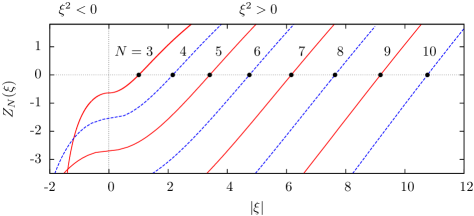
Figure 5.3: Roots $\xi_{N}$ of the function $Z_{N}(\xi)$ for boson number $N=3,\dots,10$. Only the lowest adiabatic potential (largest $\xi$) is shown.

The values are summarized in tab. 5.1 and in fig. 5.4, where we also compare with the numerical results. There is generally very good agreement between analytic and numerical results. We note that the scaling factors decrease with increasing $N$. Already for four particles it has been reduced to 4.29 as compared to 22.7. We also show the asymptotic expression for large $N$,

$$\xi_{N}=\sqrt{\frac{5}{3}N^{\frac{7}{3}}\left(1-\frac{2}{N}\right)-\frac{(3N-4)(3N-6)}{4}-\frac{1}{4}}\;,$$ (5.10)

which was established in [SSJF05a, SFJ03]. Our results are consistent with the asymptotic estimate.

N	$\xi_{N}$	$S_{N}$	$S_{N}^{2}$	$S_{N}$(SVM)
3	1.00624	22.6942	515.028	$23.6(4)\$
4	2.15584	4.29413	18.4396	$5.47(40)$
5	3.40602	2.51523	6.32638	$2.45(4)\$
6	4.74528	1.93875	3.75877	$1.93(2)\$
7	6.15939	1.66537	2.77347	$1.66(1)\$
8	7.63821	1.50878	2.27641	–
9	9.17426	1.40837	1.98352	–
10	10.7618	1.33900	1.79291	–

Table 5.1: Scaling factors $S_{N}=\exp(\pi/\xi_{N})$ for the $N$-body Efimov effect. Both analytical and numerical (SVM) results are shown. Indicated errors are from the fits in fig. 5.1. The deviation from the analytical results is largest for $N=3,4$ which use only a few states for the fit.

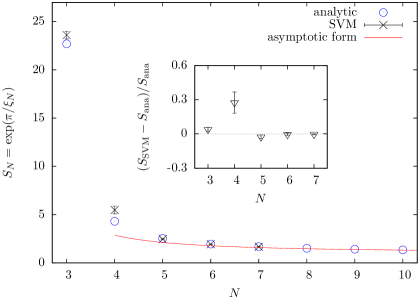
Figure 5.4: The scaling factors $S_{N}$ as function of the boson number $N$. Both analytical roots and numerical (SVM) results are shown. The $N=3$ value is the well-known factor $22.7$. The asymptotic form is given by eq. (5.10).

5.4 $N$-Body Recombination

The $N$-body Efimov states could in principle be identified by their contribution to the recombination rates in a cold gas as function of scattering length. As the scattering length is increased (using the Feshbach technique), the $N$-body Efimov states should produce peaks in the recombination rate when crossing the threshold similar to the three-body case. Such features would occur at critical scattering lengths spaced by the scaling factors $S_{N}$.

The non-resonant background rate for $N$-body recombination can be estimated as follows. Let us first consider a three-body reaction. The rate of the loss of particles from a cold gas due to the three-body recombination reaction into a shallow dimer with the energy $\hbar^{2}/(ma^{2})$ is given by Fermi’s golden rule,

$$-\frac{dN_{0}}{dt}=3\frac{N_{0}^{3}}{6}\frac{2\pi}{\hbar}\left|T_{fi}\right|^{2}\frac{d\nu_{f}}{dE_{f}},$$ (5.11)

where the factor 3 is there since each recombination reaction removes three particles from the cold gas, $N_{0}^{3}/6$ is the number of triples in the gas of $N_{0}$ particles, $d\nu_{f}$ is the number of final states (dimer plus atom) with relative momentum $q_{f}=2/(\sqrt{3}a)$ and the relative kinetic energy

$$E_{f}\equiv\frac{\hbar^{2}q_{f}^{2}}{2(\frac{2}{3}m)}=\frac{\hbar^{2}}{ma^{2}},$$ (5.12)

and $T_{fi}$ is the transition matrix element from the initial three-body state to the final atom-dimer state. The number of final states is given by

$$d\nu_{f}=\frac{Vd^{3}q_{f}}{(2\pi)^{3}}=\frac{2}{3\sqrt{3}\pi{}^{2}}\frac{Vm}{\hbar^{2}a}dE_{f}\;.$$ (5.13)

In the typical experimental regime, where the scattering length is still much smaller than the size of the trap, $a\ll b_{t}$, the transition matrix element for the non-resonant three-body recombination rate from a cold gas state into a shallow dimer state can be estimated perturbatively, substituting the asymptotic expressions for the initial and final wave-functions,

$$\begin{split}T_{fi}&=\int\,\mathrm{d}\mbox{\boldmath$r$}\,\mathrm{d}\mbox{\boldmath$R$}\left[\psi_{\mathrm{d}}(r)\frac{e^{i\mathbf{q}_{f}\mathbf{R}}}{\sqrt{V}}\right]\\ &\times\left(U(\mathbf{R}-\frac{\mathbf{r}}{2})+U(\mathbf{R}+\frac{\mathbf{r}}{2})\right)\left[\frac{e^{i\mathbf{k}\mathbf{r}}}{\sqrt{V}}\frac{e^{i\mathbf{q}\mathbf{R}}}{\sqrt{V}}\right],\end{split}$$ (5.14)

where $\mathbf{r}$ is the distance between two particles, $\mathbf{R}$ is the distance between their center-of-mass and the third particle, $V\propto b_{t}^{3}$ is the normalization volume, $k$ and $q$ ($k\sim q\propto b_{t}^{-1}\ll a^{-1}$) are the initial momenta of the cold gas particles, and $\psi_{\mathrm{d}}(r)$ is the $s$-wave function of the shallow dimer with binding energy $\hbar^{2}/(ma^{2})$. Using the zero-range approximation for the transition interaction, $U(\mathbf{r})=U_{0}\delta(\mathbf{r})$, $U_{0}=4\pi\hbar^{2}a/m$ and for the dimer wave-function, $\psi_{\mathrm{d}}(r)\propto\exp(-r/a)/(ra^{1/2})$, the matrix element eq. (5.14) in the limit $k\sim q\ll a^{-1}$ is estimated as (cf. [FRS96])

$$T_{fi}\propto\frac{\hbar^{2}a^{5/2}}{V^{3/2}m}.$$ (5.15)

Finally, the non-resonant factor of the three-body recombination rate becomes (cf. [NFJG01, FRS96])

$$\left.-\frac{dn}{dt}\right|_{\mathrm{3-body}}\propto n^{3}\frac{\hbar a^{4}}{m}\;,$$ (5.16)

where $n=N_{0}/V$ is the density.

For an $N$-body recombination reaction into a shallow $N-1$ body Efimov state with the binding energy of the order of $\hbar^{2}/(ma^{2})$ the modifications to the expression for the rate in eq. (5.11) include the extra $3(N-3)$ spatial dimensions in the integral in eq. (5.14), which gives an extra factor $(a^{3/2}V^{-1/2})^{2(N-3)}$, and also the factor $N_{0}^{3}/6$ is substituted by $N_{0}^{N}/N!$. Thus for the $N$-body recombination rate ($N\geq 3$) we have

$$\left.-\frac{dn}{dt}\right|_{\mathrm{N-body}}\propto n^{3}\frac{\hbar a^{4}}{m}(na^{3})^{N-3}\;.$$ (5.17)

We emphasize that these simple estimates only refer to the non-resonant contributions and they also do not include other types of decays where the final state structure might be substantially different from the shallow $N-1$ cluster plus one particle. The result eq. (5.17) was recently confirmed in [MRD⁺09].

Although in the regime $na^{3}\ll 1$ the $N$-body recombination has an additional small factor $(na^{3})^{N-3}$ it might still be possible to observe the $N$-body Efimov states as a sequence of resonant peaks in the recombination rate as function of scattering length, scaling as $S_{N}$.

5.5 Connection to Universal Four-Body States

Recent theoretical work [vSDG09, DvSG09, MRD⁺09] has predicted a universal four-body effect where a single atom is loosely bound to an Efimov trimer. For each trimer energy two four-body states should exist below. This leads to two extra recombination peaks at the critical scattering lengths [vSDG09]

$$a_{4B,1}\simeq 0.43a_{3B},\qquad a_{4B,2}\simeq 0.90a_{3B},$$ (5.18)

relative to the Efimov trimer resonance $a_{3B}$ (denoted $a_{Z}^{(n)}$ in chapter 2). The second state $a_{4B,2}$ is very close to the Efimov trimer. Two such features were reported experimentally in [FKB⁺09].

The universal scaling factor for this atom-Efimov effect is identical to the three-body case, i.e. $a_{4B,j}^{(n+1)}/a_{4B,j}^{(n)}=22.7$ for $j=1,2$, since these positions simply scale with the three-body states. This is different from our four-body Efimov effect which have the scaling factor $S_{4}=4.29413$. However, we note that twice the ratio of the two special four body states is $2a_{4B,2}/a_{4B,1}\simeq 4.2$. This is very close $S_{4}$ and probably within the numerical accuracy of [vSDG09]. It could indicate an underlying fundamental relationship or be a mere coincidence.

We point out that the two four-body effects are distinct, since different degrees of freedom are considered. For both of the effects the four-body states are embedded in the complete Efimov spectrum and in this respect all four-body states are meta-stable states. To treat these states as bound states one must pick out the relevant degrees of freedom, and this is where the models differ. The degrees of freedom in the atom-Efimov model is obvious, while the four-body Efimov effect presented in this chapter includes full two-body correlations.

Both effects could be relevant for Borromean four-body systems, as also pointed out in [MRD⁺09]. The connections and applications need to be explored.

5.6 Conclusions and Outlook

We have calculated the spectrum of trapped $N$-boson systems with $N=3,4,5,6,7$ using the stochastic variation method with a correlated Gaussian basis. Only two-body correlations were allowed in the variational space. Thus the cluster states were a priori mostly excluded from the variation space, which made the calculations technically possible. Inclusion of the cluster states would turn the Efimov states into meta-stable states. However the life-time of these states should be comparable with that of Bose-Einstein condensates which have similar structure and decay modes.

For each system a series of states is found with specific exponential dependence of the energies and r.m.s hyper-radii on the state number, which is a characteristic feature of Efimov states. For the $N=3$ system the obtained scaling factor agrees well with the known analytical value. We also calculated the scaling factors analytically for finite $N$ by employing a specific Faddeev-Yakubovski decomposition in two-body amplitudes. The results are in perfect agreement with the numerical results.

It might be possible to observe the four-body Efimov states as peaks in the recombination rate of a condensate as function of the scattering length, similar to the three-body case. For a dilute gas the four-body recombination rate is a factor $na^{3}$ smaller than the three-body rate, therefore the accuracy constraints on the experiment would be higher. On the other hand, the large scaling factor 22.7 for three-body recombination is reduced to 4.29 for four-body recombination. This would make the universal scaling easier to observe. The four-body case may be related to other recently investigated atom-Efimov states and could be applicable to Borromean systems.

We finally note that if the $N$-body Efimov states are found, the higher-order corrections can be derived by combining the Faddeev-Yakubovski decomposition of this chapter with the analysis of chapter 4. This would lead to shifts in the critical scattering lengths as discussed in chapter 3.

In conclusion we have lent theoretical support to the possibility of existence of long lived meta-stable $N$-body Efimov states in trapped Bose gases.

Chapter 6 Two-Body Correlations in Condensates

6.1 Introduction

The density of trapped cold gases is generally low under typical experimental conditions [PS02], such that the parameter $nr_{0}^{3}$ is small, where $n$ is the particle density and $r_{0}$ is the range of the inter-particle potential. In other words the typical distance between particles is much larger than the range of the potential, and the typical relative momentum between particles is much smaller than the inverse range of the potential.

In this regime the system of particles exhibits universality (also called model-independence or shape independence) [BH06]. The system is not sensitive to the details of the potential and the properties of the system are essentially determined by only a few low-energy parameters of the potential. Very different interaction models then provide quantitatively similar results as soon as the low-energy parameters are the same.

In a two-body system the universality is manifested in the well known effective range expansion, where the low-energy $s$-wave phase shift $\delta$ is determined by only two parameters, the scattering length $a$ and the effective range $R_{e}$, see eq. (2.4). The effective range is typically of the order of the range of the potential while the scattering length can vary greatly. In three-body systems the universality manifests itself in the Thomas collapse [Tho35], the Efimov effect [Efi70], the Phillips line [CPFG91, BHvK00, FJ02], and other low-energy phenomena [NM99], also in two dimensions [NFJ97].

Cold gases also exhibit universality: In the dilute limit their properties, in particular the energy per particle, are independent of the shape of the inter-particle potential and are determined by the scattering length alone. This universality is customarily employed by using the zero-range (pseudo) potential for theoretical descriptions of Bose-Einstein condensates. The zero-range potential has only one parameter, the scattering length. Combined with the Hartree-Fock product wave-function the zero-range potential leads to the Gross-Pitaevskii equation [DGPS99, PS03].

The limits of the zero-range model have been tested by numerical calculations with finite-range potentials. In particular, repulsive potentials have been employed with Monte-Carlo methods [BG01, GBC99, DG01] in the case of large positive scattering length. These investigations showed that as the scattering length is increased the energy of the Bose gas with a repulsive potential exceeds the zero-range predictions and the condensate fraction becomes considerably depleted.

However, repulsive potentials have a problem when modeling an increasingly large positive scattering length: The potential range, $r_{0}$, has to be increased essentially linearly with the scattering length. This does not seem to match the experimental conditions where the scattering length is adjusted by tuning the atomic resonances in an external magnetic field. The range of the inter-atomic interaction is then left essentially unchanged.

Instead, an attractive finite-range potential might be a more realistic interaction model for descriptions of trapped Bose gases with Feshbach resonances. Indeed, with an attractive potential an arbitrary large positive scattering length can be achieved by fine-tuning the energy of the bound two-body state around the threshold, while maintaining the given realistic potential range. However, attractive potentials with bound states bring in a major complication for numerical calculations: A large number of many-body self-bound negative-energy states appears in the system and the condensate state in the trap becomes a highly excited state.

For a homogeneous Bose gas an approximate Jastrow-type wave-function was employed where the pair-correlation function was essentially a solution of the two-body equation [CHM⁺02, GBC99]. In contrast we propose a direct numerical diagonalization of the many-body Hamiltonian where the condensate state of trapped bosons appears as a many-body excited state which is automatically orthogonal to all the self-bound negative-energy states. This proposal opens up the possibility to investigate the correlations which are completely absent in standard zero-range mean-field models.

When correlations are allowed in the BEC wave-function these may induce a depletion of the fully condensed state. The complete qualitative connection between the correlations and the condensate fraction still needs to be understood in detail.

The purpose of this chapter is to investigate the energy, correlations, and condensate fraction of a system of trapped bosons. The interaction is attractive and supports a single two-body state, i.e. the scattering length is positive. We will show that when the scattering length is small compared to the trap length the system is model-independent: All potential models – attractive, repulsive and zero-range – provide similar results. When the scattering length is large the attractive model differs qualitatively from the repulsive and zero-range models. In this regime the system with attractive potential becomes independent of the scattering length, with both the energy and the condensate fraction converging towards finite constants. The pair-correlation function is shown to reflect the two-body interaction at short distances and the mean-field solution at larger distances.

6.2 Condensation and Correlations

Let us start by introducing the rigorous definitions of condensation and correlations. This is done via the one-body density matrix and the two-body correlation function. The results apply to the $T=0$ formalism used in this dissertation. We also comment on some subtleties for condensation in attractive systems.

6.2.1 One-Body Density Matrix and Condensate Fraction

Assume we have a pure state described by the symmetric many-body wave-function $\Psi(\mbox{\boldmath$r$}_{1},\dots,\mbox{\boldmath$r$}_{N})$, which is normalized to $N$. The one-body density matrix (OBDM) is then defined as

$$n^{(1)}(\mbox{\boldmath$r$}_{1},\mbox{\boldmath$r$}_{1}^{\prime})=\int\Psi^{*}(\mbox{\boldmath$r$}_{1},\mbox{\boldmath$r$}_{2},\dots,\mbox{\boldmath$r$}_{N})\Psi(\mbox{\boldmath$r$}_{1}^{\prime},\mbox{\boldmath$r$}_{2},\dots,\mbox{\boldmath$r$}_{N})\,\mathrm{d}\mbox{\boldmath$r$}_{2}\dots\,\mathrm{d}\mbox{\boldmath$r$}_{N}.$$ (6.1)

The diagonal part of the OBDM is the density, $n(\mbox{\boldmath$r$})=n^{(1)}(\mbox{\boldmath$r$},\mbox{\boldmath$r$})$, which ensures that the trace equals $N$. The OBDM is hermitian so we can diagonalize it,

$$\int n(\mbox{\boldmath$r$},\mbox{\boldmath$r$}^{\prime})\chi_{i}(\mbox{\boldmath$r$}^{\prime})\,\mathrm{d}\mbox{\boldmath$r$}^{\prime}=N_{i}\chi_{i}(\mbox{\boldmath$r$}),$$ (6.2)

obtaining a complete set of orthonormal eigenfunctions $\chi_{i}(\mbox{\boldmath$r$})$ and corresponding eigenvalues $N_{i}$. The OBDM can then be expanded uniquely as

$$n(\mbox{\boldmath$r$},\mbox{\boldmath$r$}^{\prime})=\sum_{i}N_{i}\chi_{i}^{*}(\mbox{\boldmath$r$})\chi_{i}(\mbox{\boldmath$r$}^{\prime}).$$ (6.3)

The eigenvalues $N_{i}$ are non-negative, and taking the trace of the OBDM in the $\chi$-basis gives

$$\sum_{i}N_{i}=\int n(\mbox{\boldmath$r$},\mbox{\boldmath$r$})\,\mathrm{d}\mbox{\boldmath$r$}=N.$$ (6.4)

This allows us to interpret $N_{i}$ as the occupation numbers of the single particle states or natural orbitals $\chi_{i}$. We can now define a system to be a Bose-Einstein condensate if the largest eigenvalue, say $N_{0}$, is of order $N$, while all other eigenvalues are of order $1$ [PO56, Yan62]. This means that just one single-particle state, $\chi_{0}$, is macroscopically occupied. The ratio $\lambda_{0}=N_{0}/N$ is referred to as the condensate fraction.

If more than one single-particle state is macroscopically occupied, the system is called a fragmented condensate [Bay01, MHUB06]. The factorization of the OBDM into a single product $\chi^{*}(\mbox{\boldmath$r$})\chi(\mbox{\boldmath$r$}^{\prime})$ is also referred to as perfect first order coherence [NG99].

From the OBDM we can get the expectation values of all one-body observables, such as position or momentum density. Equation (6.1) can be interpreted as the amplitude to stay in the same state, if we destroy a particle at $\mbox{\boldmath$r$}_{1}^{\prime}$ and create one at $\mbox{\boldmath$r$}_{1}$. It can be related to the contrast of interference fringes measured in spatial coherence experiments [BHE00].

In practice we calculate the condensate fraction by expressing the OBDM in the harmonic oscillator basis and diagonalize numerically. Details can be found in appendix A.

6.2.2 Condensation in Attractive and Bound Systems

The definition of condensation introduced above is the conventional one. However, [WGS98] considered a gas of weakly attractive bosons in a harmonic trap with fixed angular momentum. They found that the angular momentum is absorbed by the center-of-mass motion, and that the system is fragmented, i.e. non-condensed, according to the definition used above. This is quite surprising, because the system is just a Bose-Einstein condensed ground state performing a center-of-mass motion. Ref. [PP00] then proposed an alternative definition in terms of an internal density matrix, where the center-of-mass is integrated out. According to this definition the system will be a pure condensate. However, [Gaj06] argued that the internal density matrix is only useful when describing observables that are independent of the center-of-mass. It is not useful when measuring global properties of a gas such as condensation.

These subtleties are easily explained in terms of conditional measurements. In a perfect BEC two subsequent measurements of individual particles are completely uncorrelated. The spatial probability distribution for the first particle is determined by the mean-field density, and so is the second. However if all the particles move around in a correlated way, e.g. because the system is bound, a measurement of the first particle will determine the systems center-of-mass with high accuracy. A measurement of a second particle will be close to the center-of-mass, and condensation is lost.

A concrete example on this is given in appendix B, where we show that strong hyper-radial correlation can deplete the condensate completely if the internal length scale is very different from the center-of-mass scale. Also see appendix B for a discussion on how other types of correlation affects the condensate fraction.

In the light of all these subtleties we have chosen to use the conventional criterion for Bose-Einstein condensation.

6.2.3 Two-body Correlation Function

The two-body correlation function is defined as

$$n^{(2)}(\mbox{\boldmath$r$}_{1},\mbox{\boldmath$r$}_{2})=\int\Psi^{*}(\mbox{\boldmath$r$}_{1},\mbox{\boldmath$r$}_{2},\dots,\mbox{\boldmath$r$}_{N})\Psi(\mbox{\boldmath$r$}_{1},\mbox{\boldmath$r$}_{2},\dots,\mbox{\boldmath$r$}_{N})\,\mathrm{d}\mbox{\boldmath$r$}_{3}\dots\,\mathrm{d}\mbox{\boldmath$r$}_{N},$$ (6.5)

and is interpreted as the joint probability of detecting two particles at $\mbox{\boldmath$r$}_{1}$ and $\mbox{\boldmath$r$}_{2}$ simultaneously. If the particles are totally uncorrelated the two-body correlation function factorizes as $n^{(2)}(\mbox{\boldmath$r$}_{1},\mbox{\boldmath$r$}_{2})=n(\mbox{\boldmath$r$}_{1})n(\mbox{\boldmath$r$}_{2})$. The normalized two-body correlation function is defined as

$$C^{(2)}(\mbox{\boldmath$r$}_{1},\mbox{\boldmath$r$}_{2})=\frac{n^{(2)}(\mbox{\boldmath$r$}_{1},\mbox{\boldmath$r$}_{2})}{n(\mbox{\boldmath$r$}_{1})n(\mbox{\boldmath$r$}_{2})}.$$ (6.6)

It describes the tendency of particles to cluster ($C^{(2)}>1$) or to stay separated ($0\leq C^{(2)}<1$). If no two-body correlations are present, $C^{(2)}$ equals $1$ identically.

In a homogeneous gas the correlation function (6.6) is translational invariant and depends only on $r_{12}=\lvert\mbox{\boldmath$r$}_{1}-\mbox{\boldmath$r$}_{2}\rvert$. In a spherically symmetric trap it also depends on the lengths $r_{1}$ and $r_{2}$. However, for relative distances $r_{12}$ much smaller than the density variations and the trap length, the correlation function will only depend on $r_{12}$. Thus we will typically take $\mbox{\boldmath$r$}_{2}=0$.

The correlation function in quantum gases can be measured via noise correlations [ADL04, BDZ08]. The experimental procedure is to release the gas from the trap and let it expand. The expanded density profile is then measured by light absorption imaging, and correlations in the noise are extracted. It is preferable that the gas is weakly interacting during the expansion. For Feshbach resonance experiments this is usually obtained by also ramping the scattering length down to zero when the trap is turned off.

The technique of noise correlations have recently been used to measure the correlations for fermionic gases and for bosons in optical lattices [ADL04, BDZ08], but it also works for normal trapped BECs.

6.3 System and Numerical Techniques

We consider a system of $N$ identical bosons with mass $m$ and coordinates $\mathbf{r}_{i}$, $i=1,\dots,N$, in a spherical harmonic trap with frequency $\omega$. The Hamiltonian of the system is given by eq. (2.70), where the system parameters are taken from [BG01]: $m=86.909$amu (⁸⁷Rb) and $\omega=2\pi\times 77.87$Hz, giving the trap length $b_{t}=\sqrt{\hbar/(m\omega)}=23095$au=$1.22\mu$m.

The zero-range model potential, eq. (2.59), has the scattering length $a$ as the only length parameter. For dilute bosonic systems this parameter is customarily chosen to be equal to the inter-atomic scattering length. The zero-range potential provides the correct low-energy scattering amplitude in the first order Born approximation. The zero-range potential can only be used with an appropriate non-correlated functional space, like the Hartree-Fock product wave-functions. Using the zero-range potential in a correlated space will lead to a complete Thomas collapse of the system [FJ01a].

For the finite-range potential model we use a Gaussian, eq. (2.20), with the range $r_{0}=11.65$au and a varied negative strength $V_{0}$. The variation of the strength is limited to the region where the potential provides exactly one two-body bound state and has a positive scattering length. The range of the interaction is much smaller than the trap length, i.e. $r_{0}/b_{t}=5.04\times 10^{-4}$.

Our numerical procedure is the stochastic variational method described in chapter 2. The wave-function of the system is represented as a linear combination of basis-functions taken in the form of symmetrized correlated Gaussians, eq. (2.74). The non-linear parameters $\alpha_{ij}^{(k)}$ in eq. (2.74) are optimized stochastically by random sampling from a region that covers the distances from $r_{0}$ to $b_{t}$. The center-of-mass motion is assumed to be in the oscillator’s ground state.

The zero-range potential eq. (2.59) requires an uncorrelated variational wave-function, and we use the hyper-radial wave-function $\Psi_{\rho}$ in eq. (2.75). The zero-range potential with this variational space provides results similar to the Gross-Pitaevskii equation [SFJ05].

The calculation of a highly excited state with the fully correlated basis $\Psi_{\text{full}}$, eq. (2.74), is a difficult numerical task and is only possible for relatively small number of particles. However, for a typical system of trapped atoms even when the scattering length is large the density of the system remains small, $nr_{0}^{3}\ll 1$, and one can assume that only binary collisions play a significant role in the system’s dynamics. In this approximation the variational wave-function can be simplified by only allowing two-body correlations in the basis-functions as in $\Psi_{2B}$, eq. (2.77). The symmetrization of this function can be done analytically [SFJ05] which greatly simplifies the numerical calculations.

During the calculation of a given system the number of Gaussians in the basis is increased and the stochastic optimization is carried out until the number of negative energy states and the energy of the lowest state with positive energy is converged. The convergence within four digits typically requires about $5\times 10^{2}$ Gaussian and about $10^{5}$ random trials per nonlinear parameter. When the energies are converged, the relevant properties of the wave-function can be extracted. We choose to consider densities, condensate fractions, and two-body correlation functions.

6.4 Results

6.4.1 Obtaining the BEC State

For repulsive potential models it is simply the ground state of the trapped many-boson system that is identified as the Bose-Einstein condensate (BEC) state. With deep attractive two-body potentials, however, the many-body system in a trap has a large number of self-bound negative-energy states and identification of the BEC-state is not obvious.

The typical spectrum of a trapped many-body system with attractive potentials and including two-body correlations is shown in fig. 6.1. The system has a number of deeply bound states with negative energies and then a positive quasi-continuum spectrum which starts at about $(3N/2)\hbar\omega$ and has the characteristic distance between levels of the order $\hbar\omega\ll\hbar^{2}/(2mr_{0})^{2}$. Apparently the BEC-state should then be the lowest state of the quasi-continuum spectrum or, equivalently, the lowest state with positive energy.

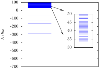
Figure 6.1: A typical spectrum (in the vicinity of zero energy) of a system of $N=20$ bosons in an oscillator trap, eq. (2.70), interacting via an attractive two-body potential, eq. (2.20), with one bound state and a positive scattering length. The inset shows the beginning of the so-called quasi-continuum spectrum.

To verify this conjecture we calculate the central density, $n_{0}$, of the system for the negative- and positive-energy states around zero energy. The results are shown in fig. 6.2 in the form of the inverse central density (the volume per particle) $n_{0}^{-1}$. In the BEC-state the atoms should occupy the whole volume of the trap and thus the volume per particle should be close to one (in the correspondingly scaled oscillator units). The states with negative energy are self-bound states with much higher density and thus much smaller volume per particle. And indeed that is what fig. 6.2 shows – a sharp increase in the volume per particle from a small value to about unity exactly at the lowest state with positive energy where the quasi-continuum starts.

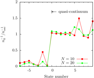
Figure 6.2: The inverse central density $n_{0}^{-1}$ (in oscillator units $n_{\mathrm{osc}}=\pi^{-3/2}Nb_{t}^{-3}$) for a system of $N$ bosons in an oscillator trap, eq. (2.70), interacting via an attractive two-body potential, eq. (2.20), with scattering length $a=119$au as function of the state number. The lowest state with positive energy is numbered zero.

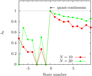
Figure 6.3: The condensate fraction of a system of $N$ trapped bosons from fig. 6.2.

Another test is the condensate fraction, shown for several states around zero energy in fig. 6.3. The self-bound states with negative energy must have smaller condensate fraction compared to the BEC-state, and the excitations from the BEC-state must gradually deplete the condensate fraction. Apparently this is what is seen in fig. 6.3 – a sharp increase of the condensate fraction to about 100% at the lowest state with positive energy with the subsequent gradual depletion.

We have thus verified that in the case of attractive potentials the BEC-state of a system of trapped bosons is the lowest state with positive energy.

6.4.2 Accuracy of the Two-Body Correlated Basis

In [BG01] the energies of several low-density systems of trapped bosons were calculated using the Gross-Pitaevskii equation as well as repulsive hard-sphere models, both with the same scattering length of 100 au. In this regime the systems exhibit universality and the energies calculated in both models were very close.

To test the accuracy of our two-body correlated basis, eq. (2.77), (which is expected to be a good approximation in the low-density regime) as well as the identification of the BEC-state for attractive potentials we consider the same systems with the same scattering length but with the attractive Gaussian potential, eq. (2.20), and calculate the energy of the BEC-state according to our prescription: The BEC-state is now an excited state and is identified in the calculations as the lowest state with positive energy. We also calculate the energies for the zero-range potential model, eq. (2.59), with the hyper-radial trial wave-function, eq. (2.75).

The results are given in tab. 6.1. As expected, these low-density systems with relatively short scattering length seem to exhibit universality as all the potential models give essentially the same results. We conclude that our identification of the BEC-state is correct and that the two-body correlated basis has an adequate accuracy.

$N$	GP$\dagger$	HS$\dagger$	ZR	A
3	4.51032	4.51036(2)	4.5103	4.510
5	7.53432	7.53443(4)	7.5342	7.534
10	15.1534	15.1537(2)	15.1533	15.154
20	30.638	30.640(1)	30.6394	30.640

• Data taken from [BG01].

Table 6.1: The energies in units of $\hbar\omega$ for the BEC-state of a system of $N$ bosons in a harmonic trap, eq. (2.70), for different interaction models with the same scattering length $a=100$au. For the Gross-Pitaevskii (GP), hard-spheres (HS), and zero-range (ZR) models the BEC-state is the ground state. For the attractive model (A) the BEC-state is the lowest state with positive energy. The zero-range model employed the hyper-radial basis, eq. (2.75), while the attractive model employed the two-body correlated basis, eq. (2.77).

To check the accuracy of the two-body correlated basis also for large scattering lengths we perform a test calculation for $N=4$ particles with fully correlated and with two-body correlated basis for vastly different scattering lengths. The results are given in tab. 6.2. Although the accuracy of the two-body correlated basis decreases somewhat with the increase of the scattering length, the relative accuracy is better than 1% even for exceedingly large scattering lengths.

$V_{0}\times 10^{7}$, au	$a$, au	$E$(2B)	$E$(full)
-1.400	119.4	6.025	6.025
-1.300	327.0	6.067	6.067
-1.290	402.4	6.083	6.083
-1.280	525.4	6.108	6.108
-1.270	761.0	6.155	6.156
-1.260	140000	6.282	6.283
-1.255	243000	6.478	6.481
-1.252	437000	6.818	6.848
-1.251	596200	7.059	7.112

Table 6.2: The energies, in units of $\hbar\omega$, of the lowest state with positive energy for a system of $N=4$ bosons in a harmonic trap, eq. (2.70). The bosons interact via an attractive Gaussian potential, eq. (2.20), with the strength $V_{0}$ and the scattering length $a$. The results from the fully correlated basis, eq. (2.74), and from the two-body correlated basis, eq. (2.77), are designated $E$(full) and $E$(2B), respectively.

6.4.3 BEC Energies

We first show the zero-range results for $N=10,100,1000$ in fig. 6.4. The energy depends on $N$ only through the combination $(N-1)a/b_{t}$ and is in perfect agreement with the Gross-Pitaevskii result. In the large $(N-1)a/b_{t}$ limit we reproduce the energy of the Thomas-Fermi limit [PS02],

$$\frac{E_{TF}}{N}=\frac{5}{14}\left(\frac{15Na}{b_{t}}\right)^{2/5}\hbar\omega.$$ (6.7)

For small $(N-1)a/b_{t}$ the interaction can be treated perturbatively: With the zero-range perturbation $H^{\prime}=\sum_{i<j}(4\pi\hbar^{2}a/m)\delta(r_{ij})$ on the non-interacting single-particle product ground state we find the energy shift

$$\frac{\Delta E}{N\hbar\omega}=\frac{1}{\sqrt{2\pi}}\frac{(N-1)a}{b_{t}}.$$ (6.8)

Our results also reproduces this regime. The agreement of our results with the GP equation was expected since both models are based on the same zero-range interaction. Also, the hyper-radial variational space for the zero-range interaction is reminiscent of the Hartree-Fock product space used in the GP equation.

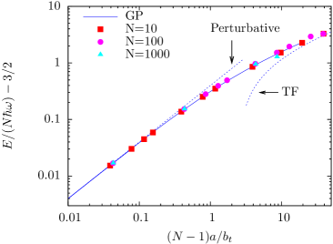
Figure 6.4: The energy per particle $E/N$ as function of the scattering length $a$ for a BEC-state of a system of $N$ identical bosons in a harmonic trap eq. (2.70) for the zero-range model eq. (2.59) (points). The results are $N$-independent in this parametrization and in perfect agreement with the Gross-Pitaevskii (GP) equation. Also shown is the perturbative and Thomas-Fermi (TF) limits, see text.

We now consider the energy per particle for the attractive potential model in fig. 6.5 and compare with the zero-range model. For small scattering lengths the different models give the same universal results – the system is model-independent. For larger scattering lengths the energies from the attractive model are systematically below the zero-range model, quite unlike the repulsive model which goes above the zero-range model [BG01, DG01]. For very large scattering lengths the attractive model, unlike the zero-range and repulsive models, becomes insensitive to the scattering length and the energies converge to a constant. This is consistent with the Jastrow-type approximation used in [CHM⁺02].

Figure 6.5: The energy per particle $E/N$ as function of the scattering length $a$ for a BEC-state of a system of $N$ trapped bosons. The results for the attractive Gaussian interaction (points) is compared with the zero-range/Gross-Pitaevskii result from fig. 6.4.

In the regime close to the two-body threshold, where the scattering length is large, an arbitrarily large change in the scattering length needs only an infinitesimally small change of the depth of the attractive potential (see tab. 6.2). Therefore, when the scattering length is larger than the trap length it ceases to be a physical length scale for the system. Since the external oscillator potential turns all continuum states into discrete states all singularities due to various thresholds are removed. Clearly an infinitesimally small change in the potential, despite the large change in the scattering length, only leads to an infinitesimal linear change in the energy which then becomes independent of the scattering length.

On the contrary, for finite-range repulsive potential models an increase of the scattering length needs an almost proportional increase in the potential range. Thus the system never ceases to depend on the scattering length.

If we plot the data using a different parametrization, namely $E$ as function of $(N-1)\left(a/b_{t}\right)^{1/2}$, the energy data points seem to follow a universal curve as shown in fig. 6.6. The specific value to which the energy converges probably depends on an independent energy scale, as for the Efimov effect in chapter 3 and 5. We speculate that other non-Gaussian interactions will reproduce the same universal curve, by tuning only a single parameter.

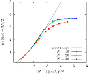
Figure 6.6: The same as is in fig. 6.5 but plotted with a different parametrization.

6.4.4 Condensate Fractions

Our results for the condensate fraction of a system of trapped identical bosons in a BEC-state are shown in fig. 6.7. For small scattering lengths the system is 100% condensate. When $(N-1)\left(a/b_{t}\right)^{1/2}$ is about 3 the condensate fraction rapidly drops a few percent before stabilizing again. Although we could not reach further due to numerical convergence problems, we expect that the condensate fraction will not appreciably change with further increase of the scattering length. This seems consistent with the energies being stagnated when approaching the two-body threshold.

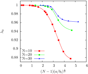
Figure 6.7: The condensate fraction of a BEC-state of a system of $N$ identical bosons in a harmonic trap eq. (2.70) with attractive inter-particle potential eq. (2.20) as function of $(N-1)(a/b_{t})^{1/2}$.

This behavior is qualitatively different from what happens within the repulsive models. In the hard-sphere Monte-Carlo simulations [DG01], the condensate fraction starts to deviate from 100% much later when $a/b_{t}$ is of the order of 0.1, and with further increase of the scattering length the condensate is completely quenched. Again our results are different from the Jastrow-type approximation [CHM⁺02], where the condensate also becomes fully quenched. However, the authors of [CHM⁺02] note that their estimates for the condensate fraction may be rather crude.

We have to note also that our wave-function includes only two-body correlations which may lead to an over-estimate of the condensate fraction.

6.4.5 Two-Body Correlation Functions

We now discuss the results for the two-body correlation function $C^{(2)}(\mbox{\boldmath$r$}_{1},\mbox{\boldmath$r$}_{2})$, eq. (6.6). For simplicity one of the coordinates is set at the center of the trap, $\mbox{\boldmath$r$}_{2}=0$. This measures the probability to find a second particle at radius $r$ when the first one is at the center. In this case the two-body correlations depend on one coordinate only, and we can easily investigate the properties over many length scales, including $r_{0}$ and $b_{t}$. However, the main conclusions will of course hold for arbitrary $\mbox{\boldmath$r$}_{2}$.

Figure 6.8 shows the two-body correlation function $C^{(2)}(r,0)$ for $N=20$ bosons in the case of an attractive Gaussian interaction with one two-body bound state ($a>0$) and two-body correlated functional space. Three different states are shown: The BEC-state determined by the lowest state in the quasi-continuum, the first state (BEC$-1$) right below the BEC-state, and the ground state.

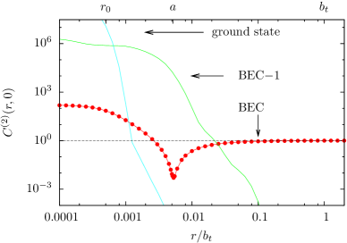
Figure 6.8: The two-body correlation function $C^{(2)}(r,0)$ for some of the different states found with the stochastic variational method. The correlation for the BEC-state (lowest state in the quasi-continuum) reflects the two-body interaction at short distances and goes to unity at large distances. The first state below the BEC-state (BEC$-1$) is self-bound and the correlation function approaches zero at large distances. This is even more pronounced for the ground state (GS).

Let us first consider the asymptotics: The correlation function for the BEC-state approaches unity for $r\to\infty$, thus the particles are completely uncorrelated at very large distances. This is what we expect, since we have shown earlier that the BEC-state has condensate fraction close to unity. The BEC$-1$ state is self-bound (bound without the trap) and hence the particles are strongly correlated. The correlation function goes to zero asymptotically, but is very large within the potential range $r_{0}$. If one particle is measured at a particular point in space it is very likely that all other particles are close to that point. Thus the state is clearly non-condensed as discussed in subsection 6.2.2.

Let us only consider the BEC-state in the rest of this chapter. We observe that the two-body correlation function in fig. 6.8 is large and positive within the range $r_{0}$ of the potential. Outside $r_{0}$ we observe a large dip in the correlation function. The value at the minimum of this dip is very small but finite. The position of the dip occurs exactly at the scattering length, $r=a$.

To understand this we consider the two-particle problem without a trap. If the two-body potential supports a single two-body bound state the relative wave-function $R(r)$ has a single node. If $a$ is larger than $r_{0}$, the position of this node is approximately at $a$. So the joint probability, and hence the two-body correlation function, is zero at the scattering length.

To investigate this in more detail we take a new two-body potential with two bound states and a large $a>0$. We calculate both the radial function $R(r)$ for the two-body problem and the correlation function for $N=20$ particles. The result is shown in fig. 6.9.

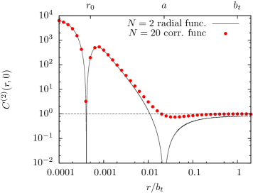
Figure 6.9: Correlation function (points) for the BEC-state of $N=20$ trapped bosons with scattering length $a$ and two bound two-body states, compared with the squared two-body zero-energy radial function $R(r)^{2}$ (line). $R$ is normalized to to match the correlation function in $r=0$

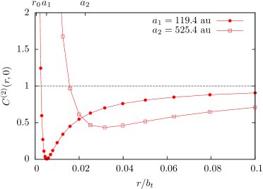
Figure 6.10: Correlation function for $N=20$ bosons in a trap. An attractive Gaussian interaction (range $r_{0}=11.65$au) was used in combination with the two-body correlated functional space. The bosons are in the BEC-state, identified as the lowest state of the quasi-continuum. Two calculations with different scattering lengths ($a_{1}$ and $a_{2}$) are shown. When the scattering length is small compared to the trap length $b_{t}$ a dip occurs at $a$. When $a$ increases the dip moves outwards and becomes shallower.

At small distances the correlation function closely follows the two-body wave-function while at large distances it converges to unity. This behavior agree well with the Jastrow product approximation used in [CHM⁺02]. We conclude that the correlation function is completely model-dependent for distances $\mbox{\boldmath$r$}_{1}-\mbox{\boldmath$r$}_{2}$ comparable to the potential range. However, for larger distances the scattering length determines the properties.

Let us now investigate the large scattering length limit, where the details are independent of the short-range potential. In fig. 6.10 the correlation function is plotted for two different scattering lengths. The $a_{1}$ data are the same as the BEC-state in fig. 6.8. When the scattering length is increased the dip moves correspondingly outwards but becomes shallower. The decrease of the dip happens since the correlated pairs starts to feel the mean-field of other particles between them. Thus the probability to find two particles within a distance $a$ is increased considerably. This is easily understood in terms of the universal shallow (Feshbach) dimers with sizes of order $a$. We conclude that in the large scattering length limit the two-body correlation function has a universal behavior. We propose to measure this effect via noise correlations as discussed earlier in this chapter.

6.5 Conclusions and Outlook

We have calculated the energy and the condensate fraction of a system of $N$ bosons in a harmonic trap as function of the number of bosons and the scattering length $a$. Specifically, we considered the regime where the scattering length is positive and comparable to the trap length. The positive scattering length is modeled using an attractive two-body potential with a bound two-body state. The many-body system then has a large number of negative-energy self-bound states and the condensate in the trap is identified as the lowest excited state with positive energy.

When the scattering length is small compared to the trap length the system shows model-independence (universality) – the results from the attractive potential model are very close to those from the zero-range and the repulsive potential models.

In the limit of large scattering length the system properties become independent of the scattering length, contrary to the zero-range and the repulsive models. For the attractive potentials the energy per particle of the system of trapped bosons tends to follow a universal curve. The condensate fraction decreases with the scattering length and reaches a finite constant at large scattering lengths contrary to the repulsive models where it reaches zero in this limit.

The two-body correlation function reflects the finite-range interaction a short distances and the mean-field solution at larger distances. When the scattering length becomes large the two-body correlations become long-ranged and universal.

In general, the stochastic variational method allows for calculations of correlations in BECs with attractive potentials. Such calculations have traditionally not been possible because of large amount of low-lying states. The obtained BEC states contain the short-range correlations while the normal mean-field features are retained. Thus, this is an important step towards understanding the non-universal corrections in condensates.

Chapter 7 Mean-Field BEC with Higher-Order Interactions

7.1 Introduction

The stability of Bose-Einstein condensates (BECs) in ultra-cold alkali gases is determined by the sign of the scattering length $a$ [DGPS99]. For $a<0$, one has effectively attractive interactions and the condensate will collapse to a dense state when the number of condensed particles, $N$, is larger than a critical number $N_{c}$ [RHBE95, BP96, DGPS99, GFT01]. This has been beautifully demonstrated in experiments with ⁷Li [BSH97], ⁸⁷Rb [RCC⁺01, DCC⁺01], and recently with a dipolar ⁵²Cr BEC [LMF⁺08]. The findings indicate that the theory based on the surprisingly simple Gross-Pitaevskii (GP) equation can reproduce and describe most features of the experiments, thus the scattering length is a universal parameter for these many-particle systems.

The GP equation includes two-body terms through a contact interaction which is parametrized by $a$. This is equivalent to a Born approximation but with an effective coupling that is obtained by replacing $a_{born}$ by the physical scattering length $a$. However, higher-order terms in the expansion of the phase shifts at low momenta, determined by the effective range $R_{e}$, the shape parameter etc., give corrections to the simple GP equation. In this chapter we explore the influence of the effective range term on the quantum properties of a BEC. In particular, we show that the critical number of condensed atoms depends strongly on the higher-order scattering term when the scattering length approaches zero (zero-crossing). We also show how the macroscopic quantum tunneling (MQT) rate, in which the entire BEC tunnels as a coherent entity, can be modified for small condensate samples.

The considered effects depend on a combination of $a$ and $R_{e}$ which yield different behavior for wide and narrow Feshbach resonances. Recent measurements on ³⁹K found many both wide and narrow resonances which allow for tuning of $a$ over many orders of magnitude [RZCD⁺07, DZF⁺07]. We therefore consider a selected example from ³⁹K in order to elucidate the general behavior for realistic experimental parameters.

In this chapter we first introduce the modified GP equation with effective range dependence. Using both a variational and numerical approach we find a phase diagram describing the stability of the condensate. We then consider an extended Feshbach resonance model including effective range variations. The behavior of the critical particle number near a scattering length zero-crossing is derived. We discuss MQT and show numerically how the rate is modified. We finally discuss other possibilities for probing the higher-order interactions.

7.2 Modified Gross-Pitaevskii Equation

We assume that the condensate can be described by the GP equation and we focus on the $a<0$ attractively interacting case. Since we are interested in the ultra-cold regime, where the temperature is much smaller than the critical temperature for condensation, we adopt the $T=0$ formalism. In order to include higher-order effects in the two-body scattering dynamics, we use the modified GP equation derived in [CMP07] for which the equivalent energy functional is

$$E(\Psi)=\int\,\mathrm{d}{\mbox{\boldmath$r$}}\left[\frac{\hbar^{2}}{2m}|\nabla\Psi|^{2}+V_{ext}(\mbox{\boldmath$r$})|\Psi|^{2}\right.\left.+\frac{U_{0}}{2}\left(|\Psi|^{4}+g_{2}|\Psi|^{2}\nabla^{2}|\Psi|^{2}\right)\right],$$ (7.1)

where $m$ is the atomic mass, $V_{ext}$ is the external trap, $U_{0}=4\pi\hbar^{2}a/m$, and $g_{2}=a^{2}/3-aR_{e}/2$ with $a$ and $R_{e}$ being the $s$-wave scattering length and effective range, respectively. The corresponding stationary GP equation found by variation of $\Psi$ is

$$\left[-\frac{\hbar^{2}}{2m}\nabla^{2}+V_{ext}(r)+U_{0}\left(|\Psi|^{2}+g_{2}\nabla^{2}|\Psi|^{2}\right)\right]\Psi=\mu\Psi,$$ (7.2)

where the chemical potential, $\mu$, was introduced to fix the particle number $N$.

7.2.1 Effective Zero-Range Interaction

To derive the modified GP equation we first need an effective two-body zero-range interaction, which by construction will give the same interaction energy as the real two-body potential. Partly following [RF01, CMP07], we first consider two non-interacting particles and restrict ourselves to $s$-waves only. In order to count energy levels and evaluate the corresponding energy shifts we choose the radial wave-function to be zero some large but arbitrary radius $L$. This gives the discrete energy levels $E_{n}=\hbar^{2}k_{n}^{2}/m$, $k_{n}=\pi n/L$ and normalized eigenstates $\psi_{n}(r)=\sqrt{2/(4\pi L)}\sin(k_{n}r)/r$. Inclusion of the true two-body interaction gives the new energy levels $\bar{E}_{n}=\hbar^{2}\bar{k}_{n}^{2}/m$ and corresponding small energy shift $\Delta E_{n}=\bar{E}_{n}-E_{n}$. The criterion

$$\Delta E_{n}=\langle\psi_{n}|\hat{V}_{ZR}|\psi_{n}\rangle$$ (7.3)

then defines the coupling constant(s) of the effective zero-range interaction $V_{ZR}$.

We first evaluate $\Delta E_{n}$. In case of interaction the asymptotic wave-function is proportional to $\sin(\bar{k}_{n}r+\delta(\bar{k}_{n}))$, where $\delta$ is the phase shift. Since the wave-function must still vanish at $L$, the wave numbers are given by $\bar{k}_{n}L=n\pi-\delta(\bar{k}_{n})$. Since $\Delta k_{n}=\bar{k}_{n}-k_{n}$ is small we have $\delta(\bar{k}_{n})\simeq\delta(k_{n})$. Using $\Delta E_{n}\simeq 2\hbar^{2}k_{n}\Delta k_{n}/m$ we find

$$\Delta E_{n}=-\frac{\delta(k_{n})}{k_{n}}\ \frac{2E_{n}}{L}.$$ (7.4)

Since we are only interested in terms up to order $k^{2}$, we use the low-energy effective range expansion

$$k\cot\delta=-\frac{1}{a}+\frac{R_{e}}{2}k^{2}+O(k^{4}),$$ (7.5)

defining the scattering length $a$ and effective range $R_{e}$. Using $\delta\simeq\tan\delta-(\tan\delta)^{3}/3$ we find

$$-\frac{\delta(k)}{k}=a\left[1-(\frac{a^{2}}{3}-\frac{aR_{e}}{2})k^{2}+O(k^{4})\right].$$ (7.6)

We now construct the zero-range interaction. The simplest hermitian ansatz up to order $k^{2}$ is $\hat{V}_{ZR}=\hat{V}_{0}+\hat{V}_{2}$ with

$$\begin{split}\hat{V}_{0}({\mbox{\boldmath$r$}})&=U_{0}\delta({\mbox{\boldmath$r$}}),\\ \hat{V}_{2}(\mbox{\boldmath$r$})&=U_{0}g_{2}\tfrac{1}{2}[\overleftarrow{\nabla}_{\mbox{\boldmath$r$}}^{2}\delta(\mbox{\boldmath$r$})+\delta(\mbox{\boldmath$r$})\overrightarrow{\nabla}_{\mbox{\boldmath$r$}}^{2}],\end{split}$$ (7.7)

where $U_{0}$ and $g_{2}$ are unknown coupling strengths to be determined from eq. (7.3). Using the non-interacting wave-functions $\psi_{n}$ we get

$$\langle\psi_{n}|\hat{V}_{ZR}|\psi_{n}\rangle=\frac{U_{0}m}{4\pi\hbar^{2}}\left(1-g_{2}k_{n}^{2}\right)\frac{2E_{n}}{L}.$$ (7.8)

Comparison of eqs. (7.4), (7.6), and (7.8) gives $U_{0}=4\pi\hbar^{2}a/m$ and $g_{2}=a^{2}/3-aR_{e}/2$. Thus we now have an effective zero-range two-body interaction to order $k^{2}$. By constructing the many-body mean-field Hamiltonian from this interaction (integrating out relative pair-distances), the last higher-order term of eq. (7.1) can be obtained [FWG03, CMP07].

7.3 Variational Calculations

We are interested in the stability properties of the ground-state and we therefore perform a variational calculation on eq. (7.1) using the mean-field trial wave-function

$$\Psi(r)=\frac{\sqrt{N}}{\pi^{3/4}\sqrt{(qb_{t})^{3}}}\exp(-\frac{r^{2}}{(qb_{t})^{2}}),$$ (7.9)

where $q$ is the dimensionless variational parameter and $b_{t}=\sqrt{\hbar/m\omega}$ is the trap length. The normalization is $N=\int\,\mathrm{d}{\mbox{\boldmath$r$}}|\Psi(r)|^{2}$. For simplicity we only consider isotropic traps with $V_{ext}(r)=\tfrac{1}{2}m\omega^{2}r^{2}$. However, the effects found should hold for deformed traps as well (along the lines of the analysis in [UL98]). The variational energy is

$$\frac{E(q)}{N\hbar\omega}=\frac{3}{4}q^{2}+\frac{3}{4}\frac{1}{q^{2}}+\frac{1}{\sqrt{2\pi}}\frac{N|a|}{b_{t}}\left(-\frac{1}{q^{3}}+3\frac{g_{2}}{b_{t}^{2}}\frac{1}{q^{5}}\right).$$ (7.10)

In fig. 7.1 we plot $E(q)$ for different parameters. As shown, there are many possibilities for $g_{2}\neq 0$, including stable, unstable, and metastable systems. We see that the $g_{2}$ term modifies the barrier for $N|a|/b_{t}=0.5$, implying that tunneling rates will be altered. For $N|a|/b_{t}=0.7$, the $g_{2}=0$ case has no barrier at all, and here the $g_{2}$ term can in fact produce a small barrier on its own. The $q^{-5}$ dependence of the term means that the effect is small. However, the plot clearly shows that a new stability analysis is needed. In addition to the variational approach we have numerically solved the full time-independent GP equation corresponding to eq. (7.1).

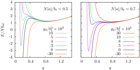
Figure 7.1: Energy of a BEC with fixed $N\lvert a\rvert/b_{t}$ as function of the variational parameter $q$, i.e. the size of the condensate. The higher-order interaction term $g_{2}$ modifies the height and shape of the barrier.

7.4 Phase Stability Diagram

To determine the ground-state stability one looks for the vanishing of the barrier towards $q=0$. For $g_{2}=0$ eq. (7.10) leads to $N_{c}|a|/b_{t}\approx 0.671$ [DGPS99]. The full integration of the GP equation gives $N_{c}|a|/b_{t}\approx k_{0}$, $k_{0}=0.5746$ [RHBE95, GFT01]. These values are indicated by filled points in fig. 7.2. The stability coefficient has been determined precisely to $0.547(58)$ using bound-state spectroscopy near a ⁸⁵Rb Feshbach resonance [CKT⁺03]. The deviation is well understood in terms of the asymmetric trap used [GFT01].

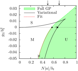
Figure 7.2: Phase stability diagram of a BEC with higher-order interactions. The solid line obtained from the variational ansatz, eq. (7.9), divides the stable (S), metastable (M), and unstable (U) regions. The white region indicates where stationary solutions exists for the full GP equation. Filled points show the well-known $g_{2}=0$ results. Arrows correspond to the values in fig. 7.1. The dashed line is the fit in eq. (7.17). Two specific ³⁹K values are chosen for zero-crossing (cross) and MQT rates (open square) calculations (see text).

In the general $g_{2}\neq 0$ case we first take the variational energy eq. (7.10) and solve for multiple roots of $\,\mathrm{d}E(q)/\,\mathrm{d}q$. The resulting “phase diagram” is plotted in fig. 7.2 (solid line). In the upper left region (S) we have complete stability of the condensate: only one minimum exists at large $q\sim 0.8$ (see fig. 7.1) and the potential goes to plus infinity at small $q$. In the metastable region (M) a barrier and a minimum exists for large $q$: for $g_{2}>0$ another minimum exists at small $q\lesssim 0.2$, while for $g_{2}<0$ the potential goes to minus infinity. In the unstable region (U) the barrier has vanished: the potential either has a minimum at small $q$ ($g_{2}>0$) or no minimum at all ($g_{2}<0$). In the variational approach the stable and unstable regions are connected via the upper right part of fig. 7.2. Going from (S) to (U) corresponds to an adiabatic change, where the macroscopic ($q\sim 1$) minimum is transferred to a microscopic ($q\ll 1$) high-density minimum.

Next, we numerically solve the full the GP equation. The stationary (white) and non-stationary (shaded) regions are shown in fig. 7.2. Since both stable and metastable solutions are considered stationary, the white region covers both (S) and (M). Both our variational and numerical results agrees with the known $g_{2}=0$ results, and have similar behavior for small and negative $g_{2}/b_{t}^{2}$.

7.5 Feshbach Resonance Model

In order to predict effects of the higher-order term, we need a realistic model for $g_{2}$. Since $g_{2}/b_{t}^{2}$ is the relevant parameter, and the trap length, $b_{t}$, is usually orders of magnitude larger than atomic scales, it is necessary to look for divergences of $g_{2}$. Since $g_{2}$ depends on $a$ and $R_{e}$, a Feshbach resonance is the obvious mean. The standard single-channel models are inadequate since only $a$ is considered.

We therefore use a multi-channel model [BJK05], which describes both $a$ and $R_{e}$ as a function of resonance position $B_{0}$, width $\Delta B$, magnetic moment difference between the channels $\Delta\mu$, and the background scattering length $a_{bg}$. In [BJK05] the on-shell $T$-matrix in the open-open channel is given by

$$\begin{split}T_{oo}&=\frac{4\pi\hbar^{2}}{m}\cdot\frac{a_{bg}}{\left(1+\frac{\Delta\mu\Delta B}{\hbar^{2}k^{2}/m-\Delta\mu(B-B_{0})}\right)^{-1}+ia_{bg}k}\\ &=\frac{4\pi\hbar^{2}}{m}\cdot\frac{1}{\frac{1}{a_{bg}}\left(1-\frac{1}{R_{e0}a_{bg}k^{2}/2+\eta}\right)^{-1}+ik},\end{split}$$ (7.11)

where $k$ is the relative momentum of the atoms and we introduced $R_{e0}=-2\hbar^{2}/ma_{bg}\Delta\mu\Delta B<0$ from eq. (2.14) and $\eta=(B-B_{0})/\Delta B$. Expanding the denominator of eq. (7.11) to second order in $k$ we get

$$T_{oo}\simeq\frac{4\pi\hbar^{2}}{m}\cdot\frac{1}{\frac{1}{a_{bg}}(1-\frac{1}{x})-\frac{R_{e0}}{2(1-\eta)^{2}}k^{2}+ik}.$$ (7.12)

By comparing this to the effective range expansion of the vacuum $T$-matrix, on-shell $T$-matrix [PS02]

$$T=-\frac{4\pi\hbar^{2}}{m}\cdot\frac{1}{k\cot\delta(k)-ik}\simeq\frac{4\pi\hbar^{2}}{m}\cdot\frac{1}{\frac{1}{a}-\frac{R_{e}}{2}k^{2}+ik},$$ (7.13)

the scattering length and effective range becomes

$$a(B)=a_{bg}\left(1-\frac{\Delta B}{B-B_{0}}\right),$$ (7.14)

$$R_{e}(B)=R_{e0}\left(1-\frac{B-B_{0}}{\Delta B}\right)^{-2}=R_{e0}\left(1-\frac{a_{bg}}{a(B)}\right)^{2}.$$ (7.15)

In [BJK05] only the regime $|B-B_{0}|\ll\Delta B$ was considered where $R_{e}\simeq R_{e0}$ is constant. The modification above includes the field dependence of $R_{e}$ and since we later want to consider a broad region around $B_{0}$ we retain this explicit field dependence.

We note that $R_{e}$ can become large (and negative) in two different ways. The first way is to consider narrow resonances where $\Delta B$ is small, and hence $R_{e0}$ is large. The other option is to tune the scattering length near a zero-crossing to small values, $a\ll a_{0}$. The effective range goes to zero far away from the resonance where $a\simeq a_{bg}$.

We now have a field-dependent $g_{2}(B)$ for given values of $B_{0}$, $\Delta B$, $\Delta\mu$, and $a_{bg}$. Notice that with this Feshbach model

$$g_{2}(a)=\frac{a^{2}}{3}-\frac{aR_{e0}}{2}\left(1-\frac{a_{bg}}{a}\right)^{2},$$ (7.16)

hence $g_{2}$ diverges when $a\to 0$ (referred to as zero-crossing) or $a\to\infty$ (on resonance). These are well-known features for model potentials like the square-well and van der Waals interactions.

As a concrete example we use the extremely narrow Feshbach resonance in ³⁹K found at $B_{0}=825$G, with $\Delta B=-0.032$G, $\Delta\mu=3.92\mu_{B}$, and $a_{bg}=-36a_{0}$ [DZF⁺07]. For this resonance we find a large $R_{e0}=-2.93\times 10^{4}a_{0}$. The variation of $a$, $R_{e}$ and $g_{2}$ as function of $B$ is shown in fig. 7.3. We use trap length $b_{t}=1.84\mu\textrm{m}=3.48\times 10^{4}a_{0}$ in all calculations unless indicated otherwise.

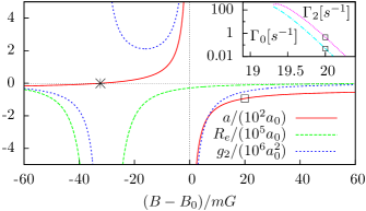
Figure 7.3: Scattering length $a$, effective range $R_{e}$, and coupling constant $g_{2}$ as function of $B$-field for the narrow ³⁹K Feshbach resonance at $B_{0}=825$ G. The inset shows the MQT rate $\Gamma_{2}$ (and $\Gamma_{0}$ for $g_{2}=0$) for $N=242$ and $b_{t}=1.84\mu$m. The cross and open square are as in fig. 7.2.

7.6 Critical Particle Number Near Zero-Crossings

As noted above, large values of $g_{2}$ are possible at zero-crossings ($a=0$) since $R_{e}$ diverges here, see e.g. fig. 7.3 around $B-B_{0}\sim-32$mG. The scattering length is currently being tuned with extreme accuracy near such zero-crossings in ⁷Li [PDJ⁺09].

The advantage is that many particles $N_{c}\propto 1/|a|$ can be accommodated in the condensate. However, for $a\rightarrow 0$ we have $ag_{2}\rightarrow-R_{e0}(a_{bg})^{2}/2$, i.e. a finite limit. Remembering that $R_{e0}$ and $\nabla^{2}|\Psi|^{2}$ are negative, the last term in the energy functional eq. (7.1) also becomes negative. Thus larger densities or density fluctuations gives lower total energy. This implies less stability and smaller $N_{c}$ near $a=0$.

To calculate quantitative effects on $N_{c}$ we focus on the critical line between the unstable and metastable regions in fig. 7.2 for $g_{2}\leq 0$. We fit the dependency as

$$N_{c}=k_{0}\frac{b_{t}}{|a|}\times\left(1-k_{1}\frac{g_{2}(a)}{b_{t}^{2}}\right)^{-1},$$ (7.17)

where $k_{1}=14.5$, as shown in fig. 7.2. With $g_{2}(a)$ given by eq. (7.16), $N_{c}$ becomes a function of $|a|/b_{t}$ for fixed values of $a_{bg}/b_{t}$ and $R_{e0}/b_{t}$. In fig. 7.4 we plot $1/N_{c}$ as function of $|a|/b_{t}$ for the ³⁹K resonance with various trap lengths. The curve deviates from the linear $g_{2}=0$ result both at $|a|\sim 0$ and $|a|\sim b_{t}$. Squeezing the trap makes the effect even more pronounced. In the limit $|a|/b_{t}\to 0$ the critical particle number approaches a finite value, $N_{c}\to 2k_{0}b_{t}^{3}/(k_{1}|R_{e0}|a_{bg}^{2})$. Large effects also occur near $|a|\sim b_{t}$, however, here the allowed particle number is very small.

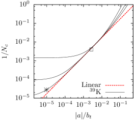
Figure 7.4: Critical particle number $N_{c}$ as function of scattering length $a$. The linear dashed (red) line is the well-known $g_{2}=0$ result $N|a|/b_{t}=k_{0}$. The solid (black) lines are for a narrow ³⁹K resonance and trap length $b_{t}=1.84\mu$m, (bottom), $0.5b_{t}$ (middle), and $0.2b_{t}$ (top). The cross and open square are as in fig. 7.2.

To exemplify with the ³⁹K resonance we use $B-B_{0}=-32.3$mG (cross in fig. 7.3) giving $a=-0.334a_{0}$ and $g_{2}/b_{t}^{2}=-0.0461$. The critical particle number is then $N_{c}=3.58\times 10^{4}$. The values are indicated by crosses in fig. 7.2 and 7.4. The $g_{2}=0$ prediction is $N_{c}=5.975\times 10^{4}$. In conclusion, we predict a 40% reduction in $N_{c}$ for macroscopic particle number $N_{c}\sim 10^{4}$.

7.7 Macroscopic Quantum Tunneling

Close to $a=\infty$, $g_{2}/b_{t}^{2}$ is still a small term in typical traps. As the MQT rate [MMT07] is exponentially dependent on the integral under the barrier, we expect changes due to non-zero $g_{2}$ to be amplified. A similar point was raised in [UL98] where the MQT rate was shown to increase dramatically close to $N_{c}$. The MQT rate, $\Gamma_{2}$, can be obtained from field theory [Sto97] by considering the bounce solution of the effective action in variational $q$-space with potential $E(q)/N\hbar\omega$. For comparison, we denote by $\Gamma_{0}$ the rate with $g_{2}=0$. All MQT calculations are done within the variational approach.

We are interested in metastable states with small barriers and large MQT rates, thus we have to work close to $N_{c}$ [UL98]. Below we find that $g_{2}/b_{t}^{2}$ is only important for the rate when $N$ is of order $10^{2}$ or less. Since the three-body loss depends on the density to the third power [Adh02], we expect it to be small in the outer metastable minimum and to be large in the inner one. Thus, the physical picture is that of a metastable BEC in the outer minimum that knocks on the barrier as a coherent state with a common quantum tunneling probability. When it tunnels to the inner minimum it swiftly decays as the large increase in density amplifies the three-body loss. Thermal fluctuations can of course also induce MQT and we therefore need to operate at very low temperature. An estimate of the thermal tunneling rate is given in [Sto97], and leads to the following criterion for thermal fluctuations to be suppressed: $E(q_{m})-E(q_{0})\gg k_{B}T$, where $q_{m}$ and $q_{0}$ are the positions of the barrier maximum and the outer minimum, respectively.

For the ³⁹K resonance we now consider $B-B_{0}=20$mG (see fig. 7.3) where $g_{2}/b_{t}^{2}=-4.3\times 10^{-4}$ and $a=-93.6a_{0}$. The critical particle number becomes $N_{c}\simeq 249$ (see fig. 7.4). We now pick $N=242<N_{c}$ to obtain metastability (see fig. 7.2). The rates are found to be $\Gamma_{2}=0.49$ s^-1 and $\Gamma_{0}=0.05$ s^-1 (shown by the open squares in the inset of fig. 7.3), i.e. a tenfold enhancement of the MQT rate. The temperature must be below 8 nK for thermal fluctuations to be small. It is possible to obtain larger $N$ with the cost of a smaller effect on the MQT rate. However, going to $N\sim 10^{3}$ does not seem possible.

We propose to start from the $a>0$ side where the condensate is stable. Preparing a sample with low enough $N$ and temperature of a few nK for the effect to be observable is the very difficult challenge for the MQT scenario. A sudden ramp of the magnetic field to the appropriate $a<0$ is then performed. The system has to retain a small barrier so that the MQT rate is considerable and to avoid collapse. Then one monitors $N$ as a function of time, as was done in e.g. [DCC⁺01]. The low $N$ is also challenging for optical imaging of the atomic cloud, but should be possible with current techniques. We expect not only to see modified MQT rates, but also changes in the decay after the condensate tunnels to a high density state: The three-body recombination is very sensitive to the density, and the inner barrier caused by the $g_{2}$ term should affect this process as well.

7.8 Other Signatures

From the structure of the $g_{2}$ term it is clear that density variations are needed to see effects. As we have demonstrated already, tighter traps amplify the contribution, and we expect optical lattices to do the same. Solitons and vortices are other features with density variation. For a simple one vortex state, the $|\Psi|^{2}\nabla^{2}|\Psi|^{2}$ term will leave the core and the asymptotic regions unchanged but change the profile in between. Work is in progress [ZT09a].

7.9 Conclusion and Outlook

We have explored the effect of higher-order terms in the Gross-Pitaevskii description of a Bose-Einstein condensate, particularly the effective range correction near a Feshbach resonance. Using both a variational and numerical approach we find an interesting new phase diagram for the stability of a condensate with negative scattering length.

The critical particle number is strongly affected near zero-crossings of the scattering length for narrow resonances. Effects of 40% are found for particle number of order $10^{4}$. These deviations increase for more narrow resonances or tighter traps. We find that the critical number will be reduced as the zero-crossing is approached from either side since the higher-order term is attractive here. Macroscopic quantum tunneling is also modified by these higher-order corrections and we have discussed some experimental conditions for exploring the physics. Narrow Feshbach resonances are the best way to isolate the effect of tunneling. However, one needs small samples of order $10^{2}$ particles or low temperatures. Other possible experimental signatures are tight traps, optical lattices, solitons, and vortices in rotating BECs.

In a more general sense, the fact that higher-order interactions can become large and dominant in determining the stability properties means that it is no longer a correction and that still higher terms might become important. This is the subject of future work. For the moment we have demonstrated that experiments targeting the regions discussed above could find interesting new stability properties beyond those that were already understood about a decade ago.

Chapter 8 Higher-Order Thomas-Fermi Approximation

8.1 Introduction

The Gross-Pitaevskii (GP) equation [DGPS99, PS02, PS03] has been extremely successful in describing a wide range of mean-field features for experiments with Bose-Einstein condensates (BECs). In particular, the Thomas-Fermi (TF) approximation [BP96, DPS96, LPS97], where the kinetic energy is neglected, has been very rewarding [VHBL⁺98]. This approximation holds for repulsive condensates with positive scattering length $a$ and large particle numbers. In the regime of validity of the TF approximation, the total energy is distributed between interaction energy and potential energy from the confining trap, while the kinetic energy becomes negligible.

Because of the non-linear nature of the GP equation, it is only solved analytically in a few cases, e.g. vortices and solitons in homogeneous condensates [PS02, PS03]. The TF solution is also analytical, although it only holds in the bulk of the condensate. At the surface the approximation breaks down and is usually patched by including the kinetic energy at the surface [DPS96, LPS97].

The interactions of the ordinary GP equation is based on the lowest order zero-range potential, which is governed by the scattering length alone. Although this approximation is usually very good, the higher-order corrections to the scattering dynamics [RF01, FWG03, CMP07] can be crucial in certain cases, e.g. for Rydberg molecules embedded in BECs [CMP07] and for narrow Feshbach resonances [ZT09b]. Inclusion of higher-order terms are well known and applied in Skyrme-Hartree-Fock calculations in nuclear physics [BGH85]. Here they often play a crucial role in order to get bulk nuclear properties right [Sky56, SJ87]. However, the effects of similar higher-order terms in the GP equation have been less investigated.

In this chapter we solve the modified GP equation with higher-order interactions analytically in the TF approximation. The chapter is organized as follows: We introduce the modified GP equation and its parameters and show how it is derived from an appropriate energy density functional with careful treatment of boundary terms. We present the analytical solution in the TF approximation and discuss the condensate size and chemical potential as function of the interaction parameters. The density profiles and energies are discussed and we address the consistency of the TF approximation by considering the kinetic energy of the solutions. We compare to some relevant atomic systems and finally present our conclusions.

8.2 Modified Gross-Pitaevskii Equation

We assume that the condensate can be described by the GP equation. Since we are interested in the ultra-cold regime, where the temperature is much smaller than the critical temperature for condensation, we adopt the $T=0$ formalism. In order to include higher-order effects in the two-body scattering dynamics we use the modified GP equation derived in [CMP07], which in the stationary form reads

$$\left[-\frac{\hbar^{2}}{2m}\nabla^{2}+V_{ext}(r)+U_{0}\left(|\Psi|^{2}+g_{2}\nabla^{2}|\Psi|^{2}\right)\right]\Psi=\mu\Psi,$$ (8.1)

where $m$ is the atomic mass, $V_{ext}$ is the external trap, $U_{0}=4\pi\hbar^{2}a/m$, and $g_{2}=a^{2}/3-aR_{e}/2$, with $a$ and $R_{e}$ being respectively the $s$-wave scattering length and effective range [CMP07]. We assume an isotropic trap, $V_{ext}(r)=m\omega^{2}r^{2}/2$, and introduce the trap length $b_{t}=\sqrt{\hbar/m\omega}$. The single-particle density, $\rho(r)=|\Psi(r)|^{2}$, is normalized to the particle number, $N=\int\,\mathrm{d}{\mbox{\boldmath$r$}}\rho(r)$, and $\mu$ is the chemical potential.

As the boundary conditions are important for the TF approximation applied below we now discuss the procedure for obtaining the modified GP equation from the corresponding energy functional which is

$$E(\Psi)=\int\,\mathrm{d}{\mbox{\boldmath$r$}}(\epsilon_{K}+\epsilon_{V}+\epsilon_{I}+\epsilon_{I2}),$$ (8.2)

with kinetic, potential and interaction energy densities

$$\epsilon_{K} =\dfrac{\hbar^{2}}{2m}|\nabla\Psi|^{2}, \epsilon_{V} =V_{ext}(\mbox{\boldmath$r$})|\Psi|^{2},$$ (8.3)

$$\epsilon_{I} =\dfrac{1}{2}U_{0}|\Psi|^{4}, \epsilon_{I2} =\dfrac{1}{2}U_{0}g_{2}|\Psi|^{2}\nabla^{2}|\Psi|^{2}.$$ (8.4)

The corresponding integrated energy contributions are denoted $E_{K}$, $E_{V}$, $E_{I}$, and $E_{I2}$ respectively. To obtain eq. (8.1), we vary eq. (8.2) with respect to $\Psi^{*}$ for fixed $\Psi$. To first order in $\delta\Psi^{*}$ we have

$$\begin{split}\delta E&=E[\Psi^{*}+\delta\Psi^{*}]-E[\Psi^{*}]\\ &=\int\,\mathrm{d}{\mbox{\boldmath$r$}}\bigg{[}-\frac{\hbar^{2}}{2m}\nabla^{2}\Psi+V_{ext}(\mbox{\boldmath$r$})\Psi+U_{0}\left(|\Psi|^{2}+g_{2}\nabla^{2}|\Psi|^{2}\right)\Psi\bigg{]}\delta\Psi^{*}\\ &+\int\,\mathrm{d}{\mbox{\boldmath$S$}}|\Psi|^{2}\nabla\left(\Psi\delta\Psi^{*}\right)-\int\,\mathrm{d}{\mbox{\boldmath$S$}}\Psi\delta\Psi^{*}\nabla|\Psi|^{2}+\int\,\mathrm{d}{\mbox{\boldmath$S$}}\delta\Psi^{*}\nabla\Psi.\end{split}$$ (8.5)

Here $S$ is the outward-pointing surface normal. In the usual analysis one assumes that $\Psi$ and $\nabla\Psi$ vanishes at infinity, drops the boundary terms, and eq. (8.1) is obtained by varying $E-\mu N$. However, the existence of these surface terms are essential for the inclusion of higher-order interactions as discussed below.

In the rest of this chapter we use trap units, $\hbar\omega=b_{t}=1$, i.e. energies ($E$, $V_{ext}$, $\mu$, etc.) are measured in units of $\hbar\omega$ and lengths ($a$, $R_{e}$, $r$, etc.) in units of $b_{t}$. Note that $g_{2}$ has dimension of length squared.

8.3 Thomas-Fermi Approximation

Let us briefly review the standard Thomas-Fermi approximation [BP96, DGPS99, PS02, PS03]. Neglecting the kinetic energy term, as compared to the trap and interaction energies, the GP equation has the solution

$$\rho_{TF}=\frac{1}{4\pi a}(\mu_{TF}-\frac{1}{2}r^{2}),$$ (8.6)

with chemical potential $\mu_{TF}$. This solution is used out to the surface, $R_{TF}$, while outside $\rho_{TF}=0$. The normalization and surface condition $\rho_{TF}(R_{TF})=0$ gives

$$\mu_{TF}=\frac{1}{2}R_{TF}^{2},\qquad R_{TF}=(15Na)^{1/5}.$$ (8.7)

The total energy becomes

$$\frac{E_{TF}}{N}=\frac{5}{7}\frac{R_{TF}^{2}}{2}.$$ (8.8)

The trap and interaction energies are $E_{V}=3E/5$ and $E_{I}=2E/5$, respectively. Since $R_{TF}>0$ in eq. (8.7), these results only hold for $a>0$. The TF approximation is good for $Na\gg 1$, except at the surface region where the kinetic energy density diverges. Here the solution can be corrected as in [DPS96, LPS97, PS02, PS03], essentially giving a small exponential tail.

8.3.1 Inclusion of Higher-Order Interactions

We now consider the TF approximation with the higher-order interaction term, $\epsilon_{I2}$. Ignoring the boundary terms in eq. (8.5), the modified GP equation can then be written in terms of the density $\rho(r)=|\Psi(r)|^{2}$ as

$${\mu}=\frac{1}{2}r^{2}+4\pi a\left(\rho+g_{2}\nabla^{2}\rho\right).$$ (8.9)

With scaled coordinate $x=r/\sqrt{g_{2}}$ (assuming $g_{2}>0$ for the moment) and density $f(r)=4\pi ax\rho(r)/g_{2}$, this becomes

$$\frac{\,\mathrm{d}^{2}f}{\,\mathrm{d}x^{2}}+f=\frac{\mu}{g_{2}}x-\frac{1}{2}x^{3},$$ (8.10)

The inhomogeneous and homogeneous solutions with boundary condition $f(0)=0$ are

$$f_{i}(x)=(\frac{\mu}{g_{2}}-\frac{1}{2}x^{2}+3)x,\quad f_{h}(x)=\frac{A}{g_{2}}\sin x,$$ (8.11)

where $A$ is a constant (with dimensions of length squared) to be determined later. The full solution is

$$\rho(x)=\frac{g_{2}}{4\pi a}\left[\frac{\mu}{g_{2}}-\frac{1}{2}x^{2}+3+\frac{A}{g_{2}}\frac{\sin x}{x}\right].$$ (8.12)

For a given $A$, the chemical potential $\mu$ and the condensate radius $R$ are determined by the normalization and the surface condition,

$$\int_{0}^{x_{0}}4\pi x^{2}\rho(x)\,\mathrm{d}r=N\quad\textrm{and}\quad\rho(x_{0})=0,$$ (8.13)

where $x_{0}=R/\sqrt{g_{2}}$. The solution $\rho$ should be positive for $x<x_{0}$ which must be explicitly checked. Outside $x_{0}$ we use $\rho=0$.

We now consider the boundary terms in eq. (8.5). Above we assumed that $\rho(x_{0})=0$ at some finite radius $x_{0}$ which we identify as the condensate size. However, only the first two boundary terms in eq. (8.5) vanish on account of this condition. For the last term in eq. (8.5) to vanish we need $\nabla_{x}\Psi(x_{0})=0$, which implies that

$$\frac{d\rho}{dx}(x_{0})=0.$$ (8.14)

Notice that this latter derivative is in fact non-zero in the $g_{2}=0$ case, which is the root of the divergence of the kinetic energy at the condensate surface as we discuss later. Equation (8.14) gives a closed expression for the remaining free parameter $A$,

$$\frac{A}{g_{2}}=\frac{x_{0}^{3}}{x_{0}\cos x_{0}-\sin x_{0}}.$$ (8.15)

This additional requirement on the derivative at the edge of the condensate implies that higher-order terms require a smoothing at the surface of the cloud. In addition, the discussion of which kinetic operator structure to use ($|\nabla\Psi|^{2}$ or $\Psi^{*}\nabla^{2}\Psi$ [LPS97]) is obsolete in our treatment since the boundary term $\delta\Psi^{*}\nabla\Psi$ vanishes. In this sense the inclusion of a higher-order term neatly removes some of the difficulties of the traditional TF treatment.

The solutions with a finite boundary $R$ of the modified GP equation only minimize the energy functional if eq. (8.14) holds. We note that extremal states of the energy functional always satisfy the virial theorem. Thus, enforcing the virial theorem on the GP solutions is equivalent to eq. (8.14). For completeness, we show in appendix C that the virial theorem approach also leads to eq. (8.15).

8.4 Size and Chemical Potential

We now determine the condensate size $R$ and chemical potential $\mu$. The normalization condition is

$$\frac{Na}{g_{2}^{5/2}}=x_{0}^{3}\left(\frac{\mu}{3g_{2}}-\frac{x_{0}^{2}}{10}\right),$$ (8.16)

while the surface condition reads

$$\frac{\mu}{g_{2}}-x_{0}^{2}/2+3+\frac{A}{g_{2}}\frac{\sin x_{0}}{x_{0}}=0.$$ (8.17)

Combining eq. (8.15), eq. (8.16), and eq. (8.17) gives

$$\frac{Na}{g_{2}^{5/2}}=x_{0}^{3}\left(\frac{x_{0}^{2}}{15}-1+\frac{x_{0}^{2}/3}{1-x_{0}\cot x_{0}}\right),$$ (8.18)

which determines $R$ for given $Na$ and $g_{2}$, and upon back-substitution also $\mu$.

The $g_{2}<0$ case can be worked out analogously by replacing trigonometric functions with hyperbolics and keeping track of signs. The two cases can in fact be combined into one equation

$$\frac{Na}{|g_{2}|^{5/2}}=|x_{0}|x_{0}^{2}\left(\frac{x_{0}^{2}}{15}-1+\frac{x_{0}^{2}/3}{1-|x_{0}\cot x_{0}|}\right).$$ (8.19)

This equation determines $x_{0}^{2}=R^{2}/g_{2}$ implicitly as function of $Na/|g_{2}|^{5/2}$. The result is shown in fig. (8.1). We notice that in principle $R$ becomes a multi-valued function. However, all the higher solutions for $g_{2}>0$ (dotted in fig. (8.1)) are spurious, since the density becomes negative on one or more intervals inside $R$. The non-spurious solutions (solid line in fig. (8.1)) defines $R$ as a single-valued function of $a$ and $g_{2}$, which was not guaranteed a priori. The four quadrants in fig. (8.1) correspond to the different sign combinations of $a$ and $g_{2}$. The sign of the extra interaction energy, $E_{I2}$, is determined by $ag_{2}\nabla^{2}\rho$. For a typical concave density the Laplacian term will be negative. We therefore see that for $ag_{2}>0$ the higher-order interaction is attractive, whereas for $ag_{2}<0$ it is repulsive. The TF solution only exists for $ag_{2}<0$. We discuss both cases separately below.

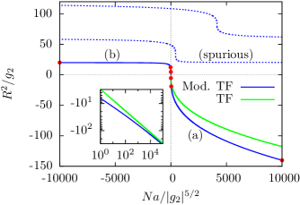
Figure 8.1: Condensate size ($R$) as function of $Na$ and $g_{2}$ as found in the modified TF approximation, eq. (8.19). The solutions (a) and (b) correspond to the sign combinations ($a>0$, $g_{2}<0$) and ($a<0$, $g_{2}>0$), respectively. No solutions exist for $ag_{2}>0$. The spurious solutions (dotted) have negative densities for one or more intervals inside $R$. The branch (a) approaches the normal TF result eq. (8.7) when $Na\to+\infty$ or $g_{2}\to-0$. Note that the convergence is only relative, see eq. (8.19), and the TF limit is better represented in the logarithmic inset. Points indicate the data from tab. (8.1). All values are in trap units.

8.4.1 The Attractive Regime: $ag_{2}>0$

For $a<0$, $g_{2}<0$ (third quadrant in fig. (8.1)) there are no solutions, which is expected since the normal TF approximation has no solutions for $a<0$ as the interaction energy $E_{I}$ is negative and the kinetic energy that could prevent collapse is neglected.

The $g_{2}>0$, $a>0$ case in the first quadrant has only spurious solutions. Here the $g_{2}$ term is attractive for the typical concave density and a collapse towards a high-density state is possible in complete analogy to the usual discussion of attractively interacting condensates within the standard GP theory. Whereas there can be metastable states at large values of $Na/g_{2}^{5/2}$, these are stabilized by kinetic energy and thus are not present in our TF approach. Thus, even when the the total kinetic energy is small, it is still needed to prevent the attractive higher-order term from amplifying local density variations.

This important point can also be established by considering the stability of the homogeneous condensate through linearization of the GP equation. By repeating the analysis of [PS02] with the higher-order term, we find that for $g_{2}>0$ and $a>0$ the kinetic energy term is crucial for the stability of the excitation modes. In fact, exponentially growing modes will always be present if the kinetic energy is neglected. This will be discussed elsewhere in relation to the numerical solution of the full GP equation [ZT09a].

8.4.2 The Repulsive Regime: $ag_{2}<0$

For $g_{2}<0$, $a>0$ a single solution (a) exists. This was expected since $E_{I2}>0$ gives extra stability. The solution approaches the normal TF result in eq. (8.7) when $Na/|g_{2}|^{5/2}\to+\infty$, as can also be seen from eq. (8.19). Of course in this limit $E_{I2}\ll E_{I}$. However, the convergence in terms of $Na/|g_{2}|^{5/2}$ is only on a relative scale, see inset in fig. (8.1) and eq. (8.19).

For $g_{2}>0$, $a<0$ there is a single solution (b) which connects smoothly to the (a) solution. In the limit $Na/|g_{2}|^{5/2}\to-\infty$, which is determined by $x_{0}\cot x_{0}=1$, we find $R^{2}/g_{2}=20.1907$. This solution is possible when the $g_{2}$ term provides just enough repulsion to cancel the usual $a<0$ collapse behavior.

8.4.3 Chemical Potential

In fig. (8.2) we show the chemical potential for the smoothly connecting solutions (a) and (b). Again we see that (a) approaches the normal TF limit for large $Na/|g_{2}|^{5/2}$. Here it is interesting to note how $\mu$ turns around near the origin (amplified in the inset in Fig (8.2)) and maintains a positive value. This occurs in the region where the lowest-order interaction gives a large negative energy contribution which the $g_{2}$ term is still able to balance yielding a well-defined TF solution. This behavior is analogues to the balancing of attraction by the kinetic term in the usual $a<0,g_{2}=0$ case [BP96, DGPS99]. As $a$ becomes increasingly negative so too does $\mu$ and collapse is inevitable (and likewise when $g_{2}\rightarrow 0^{+}$).

Figure 8.2: Chemical potential $\mu$ as function of $Na$ and $g_{2}$ as found in the modified TF approximation, using the solutions (a) and (b) from fig. (8.1). For branch (a) and the upper part of branch (b) (see inset) we have $\mu>0$. The lower part of (b) has $\mu<0$. Points indicate the data from tab. (8.1). All values are in trap units.

8.5 Densities and Energies

With $R$ and $\mu$ determined we can find the density profile, energy densities and integrated energy contributions. With eq. (8.12) the energy densities are given by

$$\epsilon_{V}=\frac{x^{2}}{2}\rho,\qquad\epsilon_{I}=2\pi a\rho^{2},\qquad\epsilon_{I2}=-\frac{1}{2}\rho(3+\frac{A}{g_{2}}\frac{\sin x}{x}).$$ (8.20)

Using eq. (8.9) the total energy density (without $\epsilon_{K}$) becomes

$$\epsilon\equiv\epsilon_{V}+\epsilon_{I}+\epsilon_{I2}=\frac{1}{2}\rho(x)(V_{ext}(x)+\frac{\mu}{g_{2}}).$$ (8.21)

In fig. (8.3) we show the density profile of the (a) solutions for $Na=10^{4}$ and selected $g_{2}<0$. We clearly see that the higher-order term tends to expand the condensate through its repulsion. Importantly, at the boundary there is a smoothing caused by the condition in eq. (8.14), see inset in fig. (8.3). We will discuss how this affects the estimated kinetic energy in the next section. As $|g_{2}|$ grows we see the condensate flatten and in the limit of very large $|g_{2}|$ it becomes a constant density.

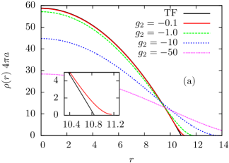
Figure 8.3: Densities for branch (a) in fig. (8.1) ($g_{2}<0$ and $Na=10^{4}$). The $g_{2}=-0.1$ curve is on top of the normal TF result. The inset shows the smooth behavior at the surface for $g_{2}<0$. All values are in trap units.

Figure (8.4) displays the density profile for the (b) solutions with $a<0$ for selected $g_{2}>0$. Here we see the profile collapse towards the expected delta-function with decreasing $g_{2}$. It is interesting to follow the (a) solution through the origin in fig. (8.1) and onto branch (b), passing from $g_{2}=-\infty$ to $g_{2}=\infty$. On the (a) branch the solution flattens as $g_{2}$ decreases and eventually becomes effectively constant in space. This is also true for the (b) branch at $g_{2}=\infty$, and as $g_{2}$ is decreased the solution proceed to shrink as the $g_{2}$ term becomes unable to provide the repulsion needed to prevent the $a<0$ collapse induced by the lowest-order term.

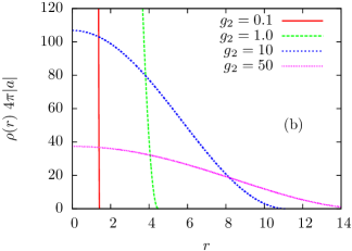
Figure 8.4: Same as fig. (8.1) but for solutions (b), i.e. opposite signs $g_{2}<0$ and $Na=-10^{4}$.

From the figures we see that large $|g_{2}|$ induces large changes in cloud size. As the condensate can be imaged with very good resolution [VHBL⁺98], this should be measurable if the regime of large $|g_{2}|$ can be accessed.

	$g_{2}$	$R$	$\mu$	$E_{V}/N$	$E_{I}/N$	$E_{I2}/N$	$E/N$	$E_{R}/N$	$E_{K}/|E|$
TF	—	10.8447	58.8040	25.2017	16.8011	—	42.0028	16.8012	3.135$\times 10^{-3}$ $\star$
	$-0.01$	10.9447	58.8188	25.2164	16.7865	0.01465	42.0176	16.8012	1.8$\times 10^{-3}$
	$-0.1$	11.1607	58.9481	25.3430	16.6635	0.13909	42.1456	16.8026	1.4$\times 10^{-3}$
(a)	$-1.0$ $\dagger$	11.8364	60.1210	26.4309	15.6818	1.16330	43.2760	16.8451	1.0$\times 10^{-3}$
	$-10$ $\dagger$	13.7835	68.4515	32.9856	11.3469	6.38609	50.7186	17.7330	0.57$\times 10^{-3}$
	$-50$ $\dagger$	16.439	87.8248	45.6836	6.99293	14.0777	66.7542	21.0706	0.30$\times 10^{-3}$
	50 $\dagger$	15.407	63.0102	38.9723	$-8.92496$	20.9439	50.9912	12.0189	0.43$\times 10^{-3}$
	10 $\dagger$	11.170	15.9128	19.8375	$-24.7434$	22.7810	17.8751	$-1.9623$	2.3$\times 10^{-3}$
(b)	5.14 $\ddagger$	9.1999	$-13.1384$	13.1579	$-46.0283$	32.8801	0.0097	$-13.148$	6.098
	1.0 $\dagger$	4.4801	$-327.612$	3.04199	$-416.359$	251.032	$-162.285$	$-165.33$	1.5$\times 10^{-3}$
	0.1	1.4204	$-10456.4$	0.30571	$-13071.1$	7842.81	$-5227.98$	$-5228.4$	0.47$\times 10^{-3}$

• The kinetic energy estimated by surface corrections as in [PS02].

• Values are indicated by points in fig. (8.1) and (8.2).

• The total energy $|E|$ is zero near $g_{2}=5.14$, hence the TF approximation is invalid here.

Table 8.1: Condensate size $R$ and chemical potential $\mu$ for different $g_{2}$ and fixed $N|a|=10^{4}$. Region (a) has $a>0$ and region (b) has $a<0$. The integrated energies are trap ($E_{V}$), interaction ($E_{I},E_{I2}$), total ($E=E_{V}+E_{I}+E_{I2}$), and release energy ($E_{R}=E-E_{V}$). The TF limit is approached for $g_{2}\to-0$. The ratio of kinetic energy $E_{K}$ to total energy $E$ indicates where the TF approximation is valid. The corresponding density distributions are shown in fig. (8.3) and (8.4). All values are in trap units.

We now discuss the energy contributions which are interesting since the release energy are in fact measurable quantities [PS03]. Since we neglect the kinetic term in the TF approximation, the release energy is simply $E_{R}=E_{I}+E_{I2}=E-E_{V}$. In tab. (8.1) we give the integrated energy contributions for some relevant values of $g_{2}$ calculated for $N|a|=10^{4}$, whereas fig. (8.5) gives the energies as function of $Na/|g_{2}|^{5/2}$. We note that for smaller values of $N|a|$ the same overall behavior is found, however, the kinetic term is more important and the TF approximation becomes worse.

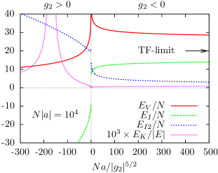
Figure 8.5: Different total energy contributions. $N|a|=10^{4}$. Values are in trap units.

We observe that $E/N$ grows towards the $|g_{2}|=\infty$ point. This is due to the trap energy increasing as the density flattens ($E_{V}$ diverges around the origin in fig. (8.5)). Furthermore, as $g_{2}\rightarrow 0^{+}$ the energy diverges towards $-\infty$ as the collapse sets in ($E_{I}$ diverges on the $g_{2}>0$ side in fig. (8.5)). The boundary where the energy vanishes is around $g_{2}=5.14$ for $N|a|=10^{4}$, but this depends on the choice of $N|a|$. With respect to the release energy, we find that somewhere in the region $10<g_{2}<50$, $E_{R}$ becomes negative. This is a result of the unavoidable collapse, and also indicates that kinetic energy cannot be ignored at this point. Notice, however, that the release energy changes considerably and could provide a way to measure the influence of the $g_{2}$ term.

8.6 Thomas-Fermi Approximation: Consistency

We now address the validity of the TF approximation with the $g_{2}$ term included. In order to do so we must consider the contribution of the kinetic energy. The kinetic energy density can be written

$$\epsilon_{K}=\frac{g_{2}}{8\rho(4\pi a)^{2}}\left(x+\frac{A}{g_{2}}\frac{x\sin x-\cos x}{x}\right)^{2}.$$ (8.22)

Strictly speaking, this is not the true kinetic energy, since the kinetic term were neglected from the start. However eq. (8.21) and eq. (8.22) can be used to test whether the TF approximation holds locally, i.e. $\epsilon_{K}\ll\epsilon$ should hold for the solution $\rho$ to be consistent. In tab. (8.1) we calculate the integrated contribution of the kinetic energy relative to the total TF energy, and we find that the contribution is small everywhere except the point where $E=0$ on the $g_{2}>0$ side of fig. (8.5). Here the kinetic energy is of course the most important term and the TF approximation is poor.

In the standard TF, the kinetic energy causes trouble at the boundary of the cloud. Here $\nabla\Psi\propto\nabla\rho/\sqrt{\rho}$ and since the density vanishes and the derivative is finite (see eq. (8.6)) this diverges at $R_{TF}$. When including the higher-order term we need to use the additional boundary condition $\nabla\Psi=0$ at $R$, so the kinetic energy will be strictly zero at $R$. However, as one approaches the boundary the kinetic energy density grows rapidly before it descends towards zero within a very small interval at $R$. The total energy density in eq. (8.21) goes to zero at this point and we find that $\epsilon_{K}/\epsilon$ is very large near the boundary as in the usual $g_{2}=0$ case.

We conclude that the inclusion of the higher-order term does not alleviate the difficulties with kinetic energy at the boundary. The techniques for addressing this problem described in [DPS96, LPS97] should therefore be generalized to include the higher-order interaction term in order to improve the description at the boundary of the cloud.

8.7 Comparison to Atomic Systems

The considerations above show that deviations from the usual TF approximation can be strong when $g_{2}$ is large. In the following we reintroduce explicit units for comparison with real systems. We have to consider $g_{2}/b_{t}^{2}$. Of course the $b_{t}^{2}$ factor means that this quantity is generally very small since $g_{2}$ is of order $a_{0}^{2}$ and $b_{t}$ is of order $10^{4}a_{0}$.

We first consider some typical background values for bosonic alkali atoms away from Feshbach resonances. We estimate the effective range to be of order the potential range, and assuming a van der Waals interaction we have $R_{e}\sim 50-200a_{0}$. For typical one-component gases we have $-450a_{0}\lesssim a\lesssim 2500a_{0}$ [CGJT09]. Since $g_{2}=a^{2}/3-aR_{e}/2$, we see that the $a^{2}$ term will dominate and in all cases $0<g_{2}\lesssim 10^{6}a_{0}$. In trap units this becomes $g_{2}/b_{t}^{2}\lesssim 5\times 10^{-3}(1\mu\text{m}/b_{t})^{2}$. In typical traps of $b_{t}\sim 1-10\mu\text{m}$ the higher-order term is therefore very small. These values also predominantly lie in the first quadrant of fig. (8.1) and thus no TF solution exists.

We now consider Feshbach resonances in order to increase the influence of the $g_{2}$ term. We use a multi-channel Feshbach model [BJK05, ZT09b], see chapter 7, which describes both $a$ and $R_{e}$ as a function of resonance position $B_{0}$, width $\Delta B$, magnetic moment difference between the channels $\Delta\mu$, and the background scattering length $a_{bg}$. We have $a=a_{bg}(1-\Delta B/(B-B_{0}))$ and $R_{e}=R_{e0}/(1-(B-B_{0})/\Delta B)^{2}$, where $R_{e0}=-2\hbar^{2}/ma_{bg}\Delta\mu\Delta B<0$. Notice that $R_{e}=R_{e0}(1-a_{bg}/a)^{2}$ and

$$g_{2}(a)=\frac{a^{2}}{3}-\frac{aR_{e0}}{2}(1-\frac{a_{bg}}{a})^{2}.$$ (8.23)

Hence $g_{2}$ diverges when $a\to 0$ (referred to as zero-crossing) or $a\to\infty$ (on resonance). Near a zero-crossing $g_{2}$ behaves as $ag_{2}\simeq|R_{e0}|a_{bg}^{2}/2$, where $R_{e0}<0$.

As a concrete example, we consider the alkali isotope ³⁹K where several Feshbach resonances of vastly different widths were found recently [DZF⁺07]. First we focus on zero-crossing and consider the very narrow resonance at $B_{0}=28.85$G with $\Delta B=-0.47$G, $\Delta\mu=1.5\mu_{B}$ and $a_{bg}=-33a_{0}$. We obtain $R_{e0}=-5687a_{0}$ and $ag_{2}\rightarrow 93.8\times 10^{3}a_{0}^{3}$ for $a\rightarrow 0$. It is important to notice that $ag_{2}>0$ around $a=0$. This means that we are looking for solutions in the first and third quadrant of fig. (8.1), and again we have to conclude that no TF solutions can be found when higher-order terms are taken into account.

Another case of interest is around resonance where $|a|=\infty$. Here we have $R_{e}\sim R_{e0}$ and $g_{2}\propto a^{2}>0$ on both sides of the resonance. Thus the $a>0$ side will be in the first and the $a<0$ in the second quadrant of fig. (8.1). This makes it difficult to imagine sweeping the resonance from either side to probe the solutions on branch (b) in fig. (8.1). One could imagine starting on the $a>0$ side with small $g_{2}>0$. The full GP equation will have perfectly sensible solution here, however, when one approaches the resonance the $g_{2}$ term will diverge and induce collapse already on the $a>0$ side. If we approach from the $a<0$ side then we face the problem that the critical number of particles decreases dramatically before $g_{2}$ grows sufficiently, and one therefore needs a very small condensate since $Na/b_{t}\sim 0.5$ [ZT09b]. At this point the TF approximation is no longer valid.

From the examples above we see considerable problems in accessing the TF solutions presented above in current experiments with ultra-cold alkali gases. In particular, we notice that realistic systems which have been used for creation of BECs in alkali gases for the last decades have parameters that predominantly lie in the first quadrant of fig. (8.1). As we have discussed there are no well-defined TF solutions in that region. Therefore we see that the kinetic energy plays a decisive role and we are forced to consider it in principle, even if it is small for all practical purposes. The physical reason is that for $a>0$ and $g_{2}>0$ the higher-order interaction is effectively attractive and induces collapse which will have to be balanced by a barrier from the kinetic term, similar to the $a<0$, $g_{2}=0$ case [DGPS99]. Since we neglect the kinetic term in the TF approximation we should not expect to find solutions in the $ag_{2}>0$ case.

8.8 Conclusion and Outlook

We have considered the effect of higher-order interactions in Bose-Einstein condensates within the Gross-Pitaevskii theory. We derived the GP equation with effective range corrections included and solved it analytically in the Thomas-Fermi approximation. Higher-order interaction terms act as derivatives on the condensate wave function which means that the boundary conditions on the solutions of the GP equation must be carefully considered. We then discussed the solutions for various parameters, presented the chemical potential, density profiles, and the energy contributions.

We find that no TF solutions are possible when the higher-order term is attractive. This conclusion holds both in the trapped system and in the homogeneous case. An estimate of the relevant parameters for alkali atoms showed, however, that they typically lie in the region where the effective range correction is effectively attractive. In order for this to be consistent with current experiments that have found the standard TF approximation to be quite good we conclude that the kinetic energy, even if very small, is crucial in order to stabilize collapse due to higher-order interaction terms. A full numerical analysis is in progress [ZT09a].

Chapter 9 Summary and Outlook

In this dissertation we presented theoretical investigations of universality and finite-range corrections in few- and many-boson systems. The main focus was on ultra-cold atomic gases seen both from the three-body, many-body, and mean-field perspective.

In the introductory chapter 1 we gave a soft introduction to the concept of universality in few- and many-body systems, in particular the wide range of effects in atomic gases and Bose-Einstein condensates. We also focused on the search for the elusive Efimov effect and its relation to nuclei and atomic gases. In chapter 2 we presented the relevant theoretical and numerical background for universal few- and many-body systems.

The purpose of chapter 3 was to go beyond the scattering length approximation for three-boson Efimov physics and express the corrections in terms of model-independent parameters. We found universal scaling with corrections determined by the effective range. We showed that for negative scattering lengths the effective range corrections to Efimov physics and Borromean binding are two aspects of the same quantitative effect. This leads to a linear shift in critical scattering lengths at the trimer threshold. For positive scattering lengths near the atom-dimer threshold the effective range corrections to the trimer energies are mainly determined by the dimer corrections. Results agree quantitatively with the newest effective field theory predictions. This has consequences for three-body recombination rates in atomic gases when the scattering length is comparable to the effective range. The main effect is that the universal scaling factor becomes smaller for the lowest Efimov states (smallest scattering length) on the negative scattering length side, corresponding to a smaller Borromean window. We also described the effects of putting the system in a finite trap.

Chapter 4 continued this line by analytically investigating the conditions for Efimov physics, in particular for large effective range. We used the adiabatic hyper-spherical approximation to derive rigorously a transcendental equation for the adiabatic potentials for general finite-range potentials. Solutions agreed with exact numerical results. We concluded that in the hyper-spherical adiabatic approximation it is insufficient to include effective range only, as another term of the same order appears. However, non-adiabatic corrections restores model-independence. For large negative effective range the window for Efimov physics is precisely open between the effective range (not the potential range) and the scattering length.

In chapter 5 we provided theoretical support for the existence of long lived meta-stable $N$-body Efimov states in atomic Bose-gases. The inclusion of two-body correlations (or equivalently a Faddeev-Yakubovski decomposition in two-body amplitudes) gave an effective hyper-radial potential as for the three-body Efimov effect. This in turn led to universal scaling, but with new scaling factors. Results were confirmed both numerically and analytically. The experimental signatures in atomic recombination experiments were discussed including possible connections to other universal four-body effects. The four-body Efimov states would be harder to detect due to the low density of experiments, but also easier to probe because of the smaller universal scaling factor. The effect could be applicable to Borromean systems too.

In chapter 6 we considered trapped few-boson systems with large positive scattering length. This was modeled using attractive two-body potentials, giving the many-body system a large amount of low-lying bound states. We presented a novel numerical technique to identify the BEC state as a highly excited many-body state. The obtained state contained short-range correlations determined by the interaction, while the normal mean-field features were retained at long distances. We found that for scattering lengths smaller than the trap the system shows universality. For larger scattering lengths the system properties becomes independent of the scattering length, contrary to the zero-range and the repulsive models. The correlations become long-ranged and universal in the large scattering length limit. This is an important step towards understanding the non-universal corrections in condensates.

Chapter 7 approached the question of effective range corrections in condensates from the mean-field point of view. A modified GP equation with effective range dependence was introduced. Using variational and numerical approaches we found a phase diagram describing the condensate stability. We then considered an extended Feshbach resonance model including effective range variations. Effects on macroscopic quantum tunneling were small for realistic systems. The behavior of the critical particle number was modified near a scattering length zero-crossing with observable consequences.

In chapter 8 we continued the mean-field analysis of the condensates using the modified Gross-Pitaevskii equation. We solved this equation analytically in Thomas-Fermi approximation where the kinetic energy can be neglected, but keeping higher-order interaction terms. Boundary conditions of the solutions were carefully considered. We presented the chemical potential, density profiles, and the energy contributions. No Thomas-Fermi solutions were possible when the higher-order term was attractive. This holds both in the trapped and homogeneous system. However, realistic atomic systems typically lie in the region where the term is attractive. In order for this to be consistent with current experiments, the kinetic energy, even if very small, is crucial in order to stabilize collapse due to higher-order interactions.

In conclusion, we have carried out new theoretical investigations of universality and its limits in few- and many-boson systems. The focus was on ultra-cold trapped atomic gases, but results were presented in universal model-independent terms. Thus, much of the work may hopefully be used or continued in other areas of physics. The subject of universality in atomic gases will face many new challenges during the next decades. Interesting new physics is clearly within reach in ultra-cold gases and indicate a promising future.

Note added.

The observation of an Efimov spectrum in an ultra-cold gas has recently been published [ZDD⁺09] giving the first definite proof of the universal scaling factors. We note that this experimental group is independent of the group measuring the first isolated Efimov state [KMW⁺06].

In [ZDD⁺09] five experimental features were found. For positive scattering length two interference minima were observed in the recombination loss rate, corresponding to two Efimov states. Also on this side two small peaks were found, corresponding to a secondary loss mechanism. For negative scattering length a single peak was found in the loss rate (the second Efimov state being out of the experimental range).

All five features agree well with the theoretical universal scaling factors except for systematic shifts. They conclude that the scaling factors are reduced on the negative scattering length side and increased on the positive side. They attribute this to finite range corrections and compare with the effects in [TFJ08c] (i.e. chapter 3) and the identical conclusions of effective field theory [PJP09]. The theory and experiment agrees. A more precise analysis is needed at this point, but the need for effective range corrections to Efimov physics is more evident now than ever before.

Appendix A Calculation of Condensate Fractions

To calculate the condensate fraction of the states found with the stochastic variational method in chapter 6 we first need to calculate the one-body density matrix (OBDM), eq. (6.1), for the two-body correlated wave-functions, eq. (2.77). We choose to change basis to the harmonic oscillator eigenfunctions before diagonalization. This basis turns out to be good, since the OBDM is almost diagonal and numerically only a few basis states are needed to ensure that the occupation numbers sum up to $N$.

Here we give an outline on how the matrix elements are calculated and the condensate fraction is obtained. First we expand the eigenfunctions of eq. (6.2) in the harmonic oscillator basis,

$$\chi_{i}(\mbox{\boldmath$r$})=\sum_{lm}a_{nlm}^{(i)}R_{nl}(r)Y_{lm}(\theta,\varphi),$$ (A.1)

$$R_{nl}(r)=\sqrt{\frac{2g^{3}n!}{\Gamma(n+l+\frac{3}{2})}}e^{-\frac{1}{2}g^{2}r^{2}}(gr)^{l}L_{n}^{l+\frac{1}{2}}(g^{2}r^{2}),$$ (A.2)

where $Y_{lm}$ are the spherical harmonics, $L_{n}^{l+\frac{1}{2}}$ are the associated (or generalized) Laguerre polynomials [AS95], and $g$ is an arbitrary oscillator scale (typically chosen as $b_{t}^{-1}$). In this basis the eigenvalue equation eq. (6.2) takes the form

$$\sum_{n^{\prime}l^{\prime}m^{\prime}}A_{nlm,n^{\prime}l^{\prime}m^{\prime}}a_{n^{\prime}l^{\prime}m^{\prime}}^{(i)}=N_{i}a_{nlm}^{(i)},$$ (A.3)

where the matrix elements are given by

$$A_{nlm,n^{\prime}l^{\prime}m^{\prime}}=\int n(\mbox{\boldmath$r$},\mbox{\boldmath$r$}^{\prime})R_{n^{\prime}l^{\prime}}(r^{\prime})R^{*}_{nl}(r)Y_{l^{\prime}m^{\prime}}(\Omega^{\prime})Y^{*}_{lm}(\Omega)\,\mathrm{d}\tau\,\mathrm{d}\tau^{\prime},$$ (A.4)

with $\,\mathrm{d}\tau=r^{2}\,\mathrm{d}r\,\mathrm{d}\Omega$. Most work lies in the evaluation of these matrix elements. It can be shown that the OBDM (in the $r$-basis) for the two-body correlated wave-function eq. (2.77) has the form

$$n(\mbox{\boldmath$r$},\mbox{\boldmath$r$}^{\prime})=\sum_{kk^{\prime}}\sum_{t=1}^{9}a^{kk^{\prime}}_{t}\exp\left(-b^{kk^{\prime}}_{t}\mbox{\boldmath$r$}^{2}-c^{kk^{\prime}}_{t}\mbox{\boldmath$r$}^{\prime 2}+d^{kk^{\prime}}_{t}\mbox{\boldmath$r$}\cdot\mbox{\boldmath$r$}^{\prime}\right).$$ (A.5)

The parameters $\{a_{t}^{kk^{\prime}},b_{t}^{kk^{\prime}},c_{t}^{kk^{\prime}},d_{t}^{kk^{\prime}}\}$ are functions of $N$ and $\{C_{k},\alpha^{(k)},\beta^{(k)}\}$. The summation over $k$ and $k^{\prime}$ corresponds to the linear-combination in eq. (2.77). The $9$ different terms labeled by $t$ comes from the symmetrization, which was done analytically. By expanding the factor $\exp(d_{t}^{kk^{\prime}}\mbox{\boldmath$r\cdot r^{\prime}$})$ in eq. (A.5) in spherical harmonics and inserting it into eq. (A.4), it is straightforward, although tedious, to calculate the matrix elements. The result is

$$\begin{split}A_{nlm,n^{\prime}l^{\prime}m^{\prime}}=&\delta_{ll^{\prime}}\delta_{mm^{\prime}}\binom{k}{n}^{\frac{1}{2}}\binom{k}{n^{\prime}}^{\frac{1}{2}}\sum_{kk^{\prime}t}a_{t}^{kk^{\prime}}\frac{(g^{2})^{3/2}x^{l}y_{+-}^{n}y_{-+}^{n^{\prime}}}{y_{++}^{3/2+l+n+n^{\prime}}}\\ &\times{}_{2}F_{1}(-n,-n^{\prime};-k;1-\frac{x^{2}}{y_{+-}y_{-+}}),\\ \end{split}$$ (A.6)

where

$$\begin{split}y_{++}=&(b_{t}^{kk^{\prime}}+g^{2}/2)(c_{t}^{kk^{\prime}}+g^{2}/2)-(d_{t}^{kk^{\prime}}/2)^{2},\\ y_{+-}=&(b_{t}^{kk^{\prime}}+g^{2}/2)(c_{t}^{kk^{\prime}}-g^{2}/2)-(d_{t}^{kk^{\prime}}/2)^{2},\\ y_{-+}=&(b_{t}^{kk^{\prime}}-g^{2}/2)(c_{t}^{kk^{\prime}}+g^{2}/2)-(d_{t}^{kk^{\prime}}/2)^{2},\\ x=&g^{2}d_{t}^{kk^{\prime}}/2,\qquad k=n+n^{\prime}+l+\frac{1}{2}.\end{split}$$ (A.7)

The hypergeometric function ${}_{2}F_{1}$ is here reducing to a Jacobi polynomium in the last argument of degree min$(n,n^{\prime})$ [AS95].

We see that $A$ is diagonal in $l$ and $m$, and also independent of $m$. This is because eq. (2.77) is rotationally invariant. We can therefore diagonalize one block at a time. The eigenvalues and eigenfunctions are re-labelled as $N_{j}^{(lm)}$ and $\chi_{j}^{(lm)}(\mbox{\boldmath$r$})$, with $j$ labeling the eigenvalues in decreasing order. The condensate fraction will usually be the first eigenvalue $\lambda_{0}=N_{0}^{(00)}/N$.

The matrix $A$ can now be diagonalized numerically and the condensate fraction obtained as the largest eigenvalue.

Appendix B Examples of Strongly Correlated Wave-Functions

The correlated wave-functions used in the stochastic variational method opens up the possibility for the condensate to be depleted considerably. It is therefore useful to know how the different types of correlations are able to lower the condensate fraction. In this appendix we give some examples of strong hyper-radial and two-body correlations.

B.1 Strong Hyper-Radial Correlation

If only one term ($k=1$) is included in the hyper-radial variational function, eq. (2.75), it reads

$$\Psi_{\rho}=c_{1}\exp\left(-\frac{NR^{2}}{2b_{t}^{2}}\right)\exp\left(-\frac{1}{2}N\alpha^{(1)}\rho^{2}\right).$$ (B.1)

In this case the occupation numbers $N_{i}$ defined in eq. (6.2) can be obtained analytically. Since we are considering a spherically symmetric trap, the total angular momentum $l$ and its projection $m$ are good quantum numbers, and we can re-label the occupation numbers as $N_{j}^{(lm)}$. The subscript $j$ labels the eigenvalues in decreasing order for given $l,m$. By expanding in the harmonic oscillator basis as in appendix A, the result is

$$N_{j}^{(lm)}=\frac{8N\xi^{l+2j}}{[1+\sqrt{1+\xi}]^{2l+4j+3}},$$ (B.2)

with

$$\xi=\frac{(\gamma-1)^{2}}{\gamma}\frac{(N-1)}{N^{2}},\qquad\gamma=N\alpha^{(1)}b_{t}^{2}.$$ (B.3)

Here $\alpha^{(1)}$ is the non-linear parameter in eq. (B.1). Note that $\gamma=1$ corresponds to the fully condensed gas where $N_{j}^{(lm)}=\delta_{j0}\delta_{l0}\delta_{m0}N$. When $\gamma$ is far away from unity the condensate fraction can be made arbitrarily small. This means that the condensate can be destroyed just because the internal length scale (measured e.g. by $\sqrt{<\rho^{2}>}$) is different from the center-of-mass length scale. This conclusion still holds for more $k$-terms in eq. (2.75). The same conclusion is also found in [Gaj06].

B.2 Strong Two-Body Correlation

To investigate the impact of two-body correlations on the condensate fraction we choose one term ($k=1$) in eq. (2.77) with $N\alpha^{(1)}b_{t}^{2}=1$. The wave-function then has the form

$$\Psi_{2B}=\prod_{i=1}^{N}\exp\left({-\frac{r_{i}^{2}}{2b_{t}^{2}}}\right)\times\hat{S}\exp\left(-\frac{1}{2}\beta^{(1)}r_{12}^{2}\right).$$ (B.4)

This is a special case of the more general form

$$\Phi=\prod_{i=1}^{N}\phi(\mbox{\boldmath$r$}_{i})\times\hat{S}f(\mbox{\boldmath$r$}_{12}),$$ (B.5)

which we will investigate instead. It is a mean-field product state modified by a correlation function. The real correlation function $f$ only includes one pair $\mbox{\boldmath$r$}_{12}$, and the function is subsequently symmetrized. We can assume without loss of generality that $\phi$ and $f$ are normalized to unity,

$$\int|\phi(\mbox{\boldmath$r$})|^{2}\,\mathrm{d}\mbox{\boldmath$r$}=\int|f(\mbox{\boldmath$r$})|^{2}\,\mathrm{d}\mbox{\boldmath$r$}=1.$$ (B.6)

We now consider the strong two-body correlated limit, where $f$ goes to zero over a range much smaller than the range over which $\phi$ varies, say

$$\begin{split}f(\mbox{\boldmath$r$})&\simeq 0\text{ for }\lvert\mbox{\boldmath$r$}\rvert>\epsilon,\\ \phi(\mbox{\boldmath$r$}+\delta\mbox{\boldmath$r$})&\simeq\phi(\mbox{\boldmath$r$})\text{ for }|\delta\mbox{\boldmath$r$}|<\epsilon.\end{split}$$ (B.7)

Here $\epsilon$ is some small length going to zero. In this limit we are able to calculate the eigenvalues and eigenfunctions of the OBDM, eq. (6.1). Since eq. (B.5) is not normalized we must first calculate the overlap integral. Because of the symmetrization in eq. (B.5) we get $[N(N-1)/2]^{2}$ terms. Many of these terms are identical, however, and only $3$ different types occur, namely

$$\langle\Phi|\Phi\rangle=N(N-1)[\langle 12|12\rangle+2(N-2)\langle 12|13\rangle+(N-2)(N-3)\langle 12|34\rangle],$$ (B.8)

where

$$\begin{split}\langle 12|12\rangle&=\int|\phi(\mbox{\boldmath$r$}_{1})|^{2}|\phi(\mbox{\boldmath$r$}_{2})|^{2}f(\mbox{\boldmath$r$}_{12})^{2}\,\mathrm{d}\mbox{\boldmath$r$}_{1}\,\mathrm{d}\mbox{\boldmath$r$}_{2}\simeq\int|\phi(\mbox{\boldmath$r$})|^{4}\,\mathrm{d}\mbox{\boldmath$r$},\\ \langle 12|13\rangle&=\int|\phi(\mbox{\boldmath$r$}_{1})|^{2}|\phi(\mbox{\boldmath$r$}_{2})|^{2}|\phi(\mbox{\boldmath$r$}_{3})|^{2}f(\mbox{\boldmath$r$}_{12})f(\mbox{\boldmath$r$}_{13})\,\mathrm{d}\mbox{\boldmath$r$}_{1}\,\mathrm{d}\mbox{\boldmath$r$}_{2}\,\mathrm{d}\mbox{\boldmath$r$}_{3}\\ &\simeq\int|\phi(\mbox{\boldmath$r$})|^{6}\,\mathrm{d}\mbox{\boldmath$r$}(\int f(\mbox{\boldmath$r$})\,\mathrm{d}\mbox{\boldmath$r$})^{2},\\ \langle 12|34\rangle&=\int|\phi(\mbox{\boldmath$r$}_{1})|^{2}|\phi(\mbox{\boldmath$r$}_{2})|^{2}|\phi(\mbox{\boldmath$r$}_{3})|^{2}\phi(\mbox{\boldmath$r$}_{4})|^{2}f(\mbox{\boldmath$r$}_{12})f(\mbox{\boldmath$r$}_{34})\,\mathrm{d}\mbox{\boldmath$r$}_{1}\,\mathrm{d}\mbox{\boldmath$r$}_{2}\,\mathrm{d}\mbox{\boldmath$r$}_{3}\,\mathrm{d}\mbox{\boldmath$r$}_{4}\\ &\simeq(\int|\phi(\mbox{\boldmath$r$})|^{4}\,\mathrm{d}\mbox{\boldmath$r$})^{2}(\int f(\mbox{\boldmath$r$})\,\mathrm{d}\mbox{\boldmath$r$})^{2}.\end{split}$$ (B.9)

The terms $\int f(\mbox{\boldmath$r$})\,\mathrm{d}\mbox{\boldmath$r$}$ are of order $\epsilon$. To lowest order in $\epsilon$ we find

$$\langle\Phi|\Phi\rangle\simeq N(N-1)\langle 12|12\rangle.$$ (B.10)

The symmetrization of the non-normalized OBDM (denoted $\tilde{n}(\mbox{\boldmath$r$},\mbox{\boldmath$r$}^{\prime})$) can be done in a similar manner. It consists of $9$ different types of terms, but to lowest order in $\epsilon$ only two terms remain,

$$\begin{split}\tilde{n}(\mbox{\boldmath$r$},\mbox{\boldmath$r$}^{\prime})=(N-1)(N-2)n_{2323}(\mbox{\boldmath$r$},\mbox{\boldmath$r$}^{\prime})+(N-1)n_{1212}(\mbox{\boldmath$r$},\mbox{\boldmath$r$}^{\prime}).\end{split}$$ (B.11)

These two terms are given by

$$\begin{split}n_{2323}(\mbox{\boldmath$r$},\mbox{\boldmath$r$}^{\prime})&=\int\phi^{*}(\mbox{\boldmath$r$})\phi(\mbox{\boldmath$r$}^{\prime})|\phi(\mbox{\boldmath$r$}_{2})|^{2}|\phi(\mbox{\boldmath$r$}_{3})|^{2}f(\mbox{\boldmath$r$}_{23})^{2}\,\mathrm{d}\mbox{\boldmath$r$}_{2}\,\mathrm{d}\mbox{\boldmath$r$}_{3}\\ &=\phi^{*}(\mbox{\boldmath$r$})\phi(\mbox{\boldmath$r$}^{\prime})\langle 12|12\rangle,\\ n_{1212}(\mbox{\boldmath$r$},\mbox{\boldmath$r$}^{\prime})&=\int\phi^{*}(\mbox{\boldmath$r$})\phi(\mbox{\boldmath$r$}^{\prime})|\phi(\mbox{\boldmath$r$}_{2})|^{2}f(\mbox{\boldmath$r$}-\mbox{\boldmath$r$}_{2})f(\mbox{\boldmath$r$}^{\prime}-\mbox{\boldmath$r$}_{2})\,\mathrm{d}\mbox{\boldmath$r$}_{2}\\ &\simeq\int|\phi(\mbox{\boldmath$s$})|^{4}f(\mbox{\boldmath$r$}-\mbox{\boldmath$s$})f(\mbox{\boldmath$r$}^{\prime}-\mbox{\boldmath$s$})\,\mathrm{d}\mbox{\boldmath$s$}.\end{split}$$ (B.12)

The normalized OBDM $n(\mbox{\boldmath$r$},\mbox{\boldmath$r$}^{\prime})=N\tilde{n}(\mbox{\boldmath$r$},\mbox{\boldmath$r$}^{\prime})/\langle\Phi|\Phi\rangle$ finally becomes

$$n(\mbox{\boldmath$r$},\mbox{\boldmath$r$}^{\prime})\simeq(N-2)\phi^{*}(\mbox{\boldmath$r$})\phi(\mbox{\boldmath$r$})+\int\!\,\mathrm{d}\mbox{\boldmath$s$}\,N_{\mbox{\boldmath$s$}}\,\chi^{*}_{\mbox{\boldmath$s$}}(\mbox{\boldmath$r$})\,\chi_{\mbox{\boldmath$s$}}(\mbox{\boldmath$r$}^{\prime}),$$ (B.13)

where we have defined

$$\chi_{\mbox{\boldmath$s$}}(\mbox{\boldmath$r$})=f(\mbox{\boldmath$r$}-\mbox{\boldmath$s$}),\qquad N_{\mbox{\boldmath$s$}}=2\frac{n(\mbox{\boldmath$s$})^{2}}{\int n(\mbox{\boldmath$r$})^{2}\,\mathrm{d}\mbox{\boldmath$r$}}.$$ (B.14)

Here $n(\mbox{\boldmath$r$})=\lvert\phi(\mbox{\boldmath$r$})\rvert^{2}$ is the mean-field density. Notice that eq. (B.13) has trace equal to $N$. The set $\{\phi,\chi_{\mbox{\boldmath$s$}}|\mbox{\boldmath$s$}\in\mathbb{R}^{3}\}$ is orthonormal in the limit considered. Since the expansion of the OBDM in eigenfunctions, eq. (6.3), is unique, we can compare eq. (6.3) with eq. (B.13) and read off eigenfunctions and corresponding eigenvalues directly. The condensate fraction is reduced to $1-2/N$ with $\phi$ still being the corresponding single-particle state. The remaining $2$ “particles” are distributed over infinitely many states $\chi_{\mbox{\boldmath$s$}}(\mbox{\boldmath$r$})$, which are peaked around $s$. The occupation numbers $\,\mathrm{d}\mbox{\boldmath$s$}\,N_{\mbox{\boldmath$s$}}$ for $\chi_{\mbox{\boldmath$s$}}(\mbox{\boldmath$r$})$ are proportional to the square-density, $n(\mbox{\boldmath$s$})^{2}$, of the mean-field.

Appendix C TF Boundary Conditions and the Virial Equation

In this appendix we derive the free parameter $A$ of the Thomas-Fermi solution eq. (8.12) in chapter 8. This is done explicitly by enforcing the virial equation. We show that this is equivalent to the boundary condition eq. (8.14).

Even though eq. (8.12) is a solution to the modified GP equation eq. (8.9) for all $A$, it does not necessarily minimize the energy functional as discussed in the section 8.3. This can also be seen from the virial equation (with neglected kinetic energy),

$$-2E_{V}+3E_{I}+5E_{I2}=0,$$ (C.1)

which holds for all extremal points of the energy functional. Equation (C.1) is derived from the energy functional using scaling arguments as in [PS03].

As an example consider the $A=0$ solution in eq. (8.12). This solution has a chemical potential shifted by $3g_{2}$ compared to the $g_{2}=0$ TF result. But the density is unchanged and so is $E_{V}$ and $E_{I}$. Hence the usual virial equation $-2E_{V}+3E_{I}=0$ for $g_{2}=0$ also holds for $g_{2}\neq 0$. Since $E_{I2}=-3g_{2}/2\neq 0$ the virial equation eq. (C.1) is not fulfilled, and hence the $A=0$ solution is not extremal. Below we use the virial equation to calculate the value of $A$ that minimizes the energy functional and the corresponding $R$ and $\mu$. We will also prove that this condition is in fact equivalent to assume $\rho(x_{0})=\nabla_{x}\rho(x_{0})=0$ at the boundary.

The general results for $A$, $R$, and $\mu$ can be derived using the normalization and surface conditions eq. (8.13), and the virial equation eq. (C.1). For convenience we introduce the variables $\bar{\mu}=\mu/(3g_{2})+1$, $\bar{A}=A/(3g_{2})$, and $c=Na/g_{2}^{5/2}$. The different energy contributions are

$$\begin{split}E_{V}&=3s\int_{0}^{x_{0}}\,\mathrm{d}xx^{4}(\bar{\mu}-\frac{x^{2}}{6}+\bar{A}\frac{\sin x}{x}),\\ E_{I}&=9s\int_{0}^{x_{0}}\,\mathrm{d}xx^{2}(\bar{\mu}-\frac{x^{2}}{6}+\bar{A}\frac{\sin x}{x})^{2},\\ E_{I2}&=-9s\int_{0}^{x_{0}}\,\mathrm{d}xx^{2}(\bar{\mu}-\frac{x^{2}}{6}+\bar{A}\frac{\sin x}{x})(1+\bar{A}\frac{\sin x}{x}),\end{split}$$ (C.2)

where $s=g_{2}^{7/2}/(2a)$. Direct integration of eq. (C.2), insertion of $\bar{\mu}$ from the normalization eq. (8.17), and some algebra gives the virial equation

$$\begin{split}0&=-2E_{V}+3E_{I}+5E_{I2}\\ &=-\frac{s}{x_{0}}(x_{0}^{3}-3\bar{A}(x_{0}\cos x_{0}-\sin x_{0}))^{2}.\end{split}$$ (C.3)

We immediately see that this is in fact equivalent to eq. (8.15). Therefore, the solution we have explicitly found above minimizes the energy functional with boundary conditions $\rho(x_{0})=\nabla_{x}\rho(x_{0})=0$. More generally, when we solved the MGP without considering the boundary terms in section (8.3), we found a one-parameter family of solutions (parametrized by $A$). The virial theorem is merely a constraint on $A$ for obtaining a minimum of $E$.

References

- [FJT08] D. V. Fedorov, A. S. Jensen, and M. Thøgersen, Bose-Einstein condensates and Efimov states in trapped many-boson systems, Few-Body Sys., 43 (2008) 69.
- [FJT+09] D. V. Fedorov, A. S. Jensen, M. Thøgersen, E. Garrido, and R. de Diego, Calculating few-body resonances using an oscillator trap, Few-Body Sys., 45 (2009) 191.
- [JKTF07] A. S. Jensen, T. Kjærgaard, M. Thøgersen, and D. V. Fedorov, Eigenvalues of the one-body density matrix for correlated condensates, Nucl. Phys. A, 790 (2007) 723c.
- [TFJ07] M. Thøgersen, D. V. Fedorov, and A. S. Jensen, Trapped Bose gases with large positive scattering length, Europhys. Lett., 79 (2007) 40002.
- [TFJ08a] M. Thøgersen, D. V. Fedorov, and A. S. Jensen, -body Efimov states of trapped bosons, Europhys. Lett., 83 (2008) 30012.
- [TFJ08b] M. Thøgersen, D. V. Fedorov, and A. S. Jensen, Spatial correlations in Bose gases, AIP Conf. Proc., 998 (2008) 85.
- [TFJ08c] M. Thøgersen, D. V. Fedorov, and A. S. Jensen, Universal properties of Efimov physics beyond the scattering length approximation, Phys. Rev. A, 78 (2008) 020501(R).
- [TFJ+09] M. Thøgersen, D. V. Fedorov, A. S. Jensen, B. D. Esry, and Y. Wang, Conditions for Efimov physics for finite range potentials, Phys. Rev. A, 80 (2009) 013608.
- [TZJ09] M. Thøgersen, N. Zinner, and A. S. Jensen, Thomas-Fermi approximation for a condensate with higher-order interactions, Submitted to Phys. Rev. A, arXiv:0907.5349 [cond-mat.quant-gas].
- [ZT09a] N. Zinner and M. Thøgersen, Higher-order terms in an attractively interacting BEC: Mean-field stability and macroscopic tunneling lifetimes, In preparation.
- [ZT09b] N. Zinner and M. Thøgersen, Stability of a Bose-Einstein condensate with higher-order interactions near a Feshbach resonance, Phys. Rev. A (in press), arXiv:0903.2261v2 [cond-mat.other].

References

- [Adh02] S. K. Adhikari, Mean-field description of collapsing and exploding Bose-Einstein condensates, Phys. Rev. A, 66 (2002) 013611.
- [ADL04] E. Altman, E. Demler, and M. D. Lukin, Probing many-body states of ultracold atoms via noise correlations, Phys. Rev. A, 70 (2004) 013603.
- [AEM+95] M. H. Anderson, J. R. Ensher, M. R. Matthews, C. E. Wieman, and E. A. Cornell, Observation of Bose-Einstein condensation in a dilute atomic vapor, Science, 269 (1995) 198.
- [AFT97] A. E. A. Amorim, T. Frederico, and L. Tomio, Universal aspects of Efimov states and light halo nuclei, Phys. Rev. C, 56 (1997) 2378(R).
- [AG73] R. D. Amado and F. C. Greenwood, There is no Efimov effect for four or more particles, Phys. Rev. D, 7 (1973) 2517.
- [AN71] R. D. Amado and J. V. Noble, On Efimov’s effect: A new pathology of three-particle systems, Phys. Lett. B, 35 (1971) 25.
- [AN72] R. D. Amado and J. V. Noble, Efimov’s effect: A new pathology of three-particle systems. II, Phys. Rev. D, 5 (1972) 1992.
- [AS95] M. Abramowitz and I. A. Stegun (eds.), Handbook of Mathematical functions, Dover, New York, 9th ed. (1995).
- [ASRVK01] J. R. Abo-Shaeer, C. Raman, J. M. Vogels, and W. Ketterle, Observation of vortex lattices in Bose-Einstein condensates, Science, 292 (2001) 476.
- [ATM+97] M. R. Andrews, C. G. Townsend, H.-J. Miesner, D. S. Durfee, D. M. Kurn, and W. Ketterle, Observation of interference between two Bose condensates, Science, 275 (1997) 637.
- [Bay01] G. Baym, Topics in the microscopic theory of Bose-Einstein condensates, J. Phys. B, 34 (2001) 4541.
- [BDZ08] I. Bloch, J. Dalibard, and W. Zwerger, Many-body physics with ultracold gases, Rev. Mod. Phys., 80 (2008) 885.
- [BG01] D. Blume and C. H. Greene, Quantum corrections to the ground-state energy of a trapped Bose-Einstein condensate: A diffusion Monte Carlo calculation, Phys. Rev. A, 63 (2001) 063601.
- [BGH85] M. Brack, C. Guet, and H. B. Håkansson, Selfconsistent semiclassical description of average nuclear properties–a link between microscopic and macroscopic models, Phys. Rep., 123 (1985) 275.
- [BH03] E. Braaten and H.-W. Hammer, Universality in the three-body problem for 4He atoms, Phys. Rev. A, 67 (2003) 042706.
- [BH06] E. Braaten and H.-W. Hammer, Universality in few-body systems with large scattering length, Phys. Rep., 428 (2006) 259.
- [BHE00] I. Bloch, T. W. Hänsch, and T. Esslinger, Measurement of the spatial coherence of a trapped Bose gas at the phase transition, Nature, 403 (2000) 166.
- [BHK03] E. Braaten, H.-W. Hammer, and M. Kusunoki, Universal equation for Efimov states, Phys. Rev. A, 67 (2003) 022505.
- [BHvK00] P. F. Bedaque, H. W. Hammer, and U. van Kolck, Effective theory of the triton, Nucl. Phys. A, 676 (2000) 357.
- [BJ03] B. H. Bransden and C. J. Joachain, Physics of Atoms and Molecules, Pearson Education, 2nd ed. (2003).
- [BJK05] G. M. Bruun, A. D. Jackson, and E. E. Kolomeitsev, Multichannel scattering and Feshbach resonances: Effective theory, phenomenology, and many-body effects, Phys. Rev. A, 71 (2005) 052713.
- [BKK+05] R. Brühl, A. Kalinin, O. Kornilov, J. P. Toennies, G. C. Hegerfeldt, and M. Stoll, Matter wave diffraction from an inclined transmission grating: Searching for the elusive 4He trimer Efimov state, Phys. Rev. Lett., 95 (2005) 063002.
- [BP96] G. Baym and C. J. Pethick, Ground-state properties of magnetically trapped Bose-condensed rubidium gas, Phys. Rev. Lett., 76 (1996) 6.
- [BSH97] C. C. Bradley, C. A. Sackett, and R. G. Hulet, Bose-Einstein condensation of lithium: Observation of limited condensate number, Phys. Rev. Lett., 78 (1997) 985.
- [CGJT09] C. Chin, R. Grimm, P. Julienne, and E. Tiesinga, Feshbach resonances in ultracold gases, arXiv:0812.1496v2 [cond-mat.other].
- [CHM+02] S. Cowell, H. Heiselberg, I. E. Mazets, J. Morales, V. R. Pandharipande, and C. J. Pethick, Cold Bose gases with large scattering lengths, Phys. Rev. Lett., 88 (2002) 210403.
- [CKR+07] M. Combescure, A. Khare, A. K. Raina, J.-M. Richard, and C. Weydert, Level rearrangement in exotic atoms and quantum dots, Int. J. Mod. Phys. B, 21 (2007) 3765.
- [CKT+03] N. R. Claussen, S. J. J. M. F. Kokkelmans, S. T. Thompson, E. A. Donley, E. Hodby, and C. E. Wieman, Very-high-precision bound-state spectroscopy near a 85Rb Feshbach resonance, Phys. Rev. A, 67 (2003) 060701.
- [CMP07] A. Collin, P. Massignan, and C. J. Pethick, Energy-dependent effective interactions for dilute many-body systems, Phys. Rev. A, 75 (2007) 013615.
- [CPFG91] C. R. Chen, G. L. Payne, J. L. Friar, and B. F. Gibson, Nd zero-energy scattering, Phys. Rev. C, 44 (1991) 50.
- [Dan61] G. S. Danilov, On the three-body problem in the case of short-range forces, Zh. Eksp. Teor. Fiz., 40 (1961) 498.
- [DCC+01] E. A. Donley, N. R. Claussen, S. L. Cornish, J. L. Roberts, E. A. Cornell, and C. E. Wieman, Dynamics of collapsing and exploding Bose-Einstein condensates, Nature, 412 (2001) 295.
- [DE05] J. P. D’Incao and B. D. Esry, Scattering length scaling laws for ultracold three-body collisions, Phys. Rev. Lett., 94 (2005) 213201.
- [DE06] J. P. D’Incao and B. D. Esry, Enhancing the observability of the Efimov effect in ultracold atomic gas mixtures, Phys. Rev. A, 73 (2006) 030703.
- [DG01] J. L. DuBois and H. R. Glyde, Bose-Einstein condensation in trapped bosons: A variational Monte Carlo analysis, Phys. Rev. A, 63 (2001) 023602.
- [DGPS99] F. Dalfovo, S. Giorgini, L. P. Pitaevskii, and S. Stringari, Theory of Bose-Einstein condensation in trapped gases, Rev. Mod. Phys., 71 (1999) 463.
- [DPS96] F. Dalfovo, L. Pitaevskii, and S. Stringari, Order parameter at the boundary of a trapped Bose gas, Phys. Rev. A, 54 (1996) 4213.
- [DRN07] A. M. Dudarev, M. G. Raizen, and Q. Niu, Quantum many-body culling: Production of a definite number of ground-state atoms in a Bose-Einstein condensate, Phys. Rev. Lett., 98 (2007) 063001.
- [DvSG09] J. P. D’Incao, J. von Stecher, and C. H. Greene, Universal four-boson states in ultracold molecular gases: Resonant effects in dimer-dimer collisions, Phys. Rev. Lett., 103 (2009) 033004.
- [DZF+07] C. D’Errico, M. Zaccanti, M. Fattori, G. Roati, M. Inguscio, G. Modugno, and A. Simoni, Feshbach resonances in ultracold 39K, New J. Phys., 9 (2007) 223.
- [Efi70] V. Efimov, Energy levels arising from resonant two-body forces in a three-body system., Phys. Lett. B, 33 (1970) 563.
- [Efi71] V. N. Efimov, Weakly-bound states of three resonantly-interacting particles, Sov. J. Nucl. Phys., 12 (1971) 589.
- [Efi73] V. Efimov, Energy levels of three resonantly interacting particles, Nucl. Phys. A, 210 (1973) 157.
- [Efi90] V. Efimov, Is a qualitative approach to the three-body problem useful?, Comm. Nucl. Part. Phys., 19 (1990) 271.
- [Efi91] V. Efimov, Force-range correction in the three-body problem: Application to three-nucleon systems, Phys. Rev. C, 44 (1991) 2303.
- [EG06] B. D. Esry and C. H. Greene, Quantum physics: A ménage à trois laid bare, Nature, 440 (2006) 289.
- [EGB99] B. D. Esry, C. H. Greene, and J. P. Burke, Recombination of three atoms in the ultracold limit, Phys. Rev. Lett., 83 (1999) 1751.
- [Ein24] A. Einstein, Quantum theory of monatomic ideal gases, Sitzungsberichte der Preussichen Akademie der Wissenschaften Physikalisch-Mathematische Klasse (1924) 261.
- [ELG96] B. D. Esry, C. D. Lin, and C. H. Greene, Adiabatic hyperspherical study of the helium trimer, Phys. Rev. A, 54 (1996) 394.
- [FJ93] D. V. Fedorov and A. S. Jensen, Efimov effect in coordinate space Faddeev equations, Phys. Rev. Lett., 71 (1993) 4103.
- [FJ01a] D. V. Fedorov and A. S. Jensen, Correlation-induced collapse of many-body systems with zero-range potentials, Phys. Rev. A, 63 (2001) 063608.
- [FJ01b] D. V. Fedorov and A. S. Jensen, Regularization of a three-body problem with zero-range potentials, J. Phys. A, 34 (2001) 6003.
- [FJ02] D. V. Fedorov and A. S. Jensen, Regularized zero-range model and an application to the triton and the hypertriton, Nucl. Phys. A, 697 (2002) 783.
- [FJR94] D. V. Fedorov, A. S. Jensen, and K. Riisager, Efimov states in halo nuclei, Phys. Rev. Lett., 73 (1994) 2817.
- [FJT08] D. V. Fedorov, A. S. Jensen, and M. Thøgersen, Bose-Einstein condensates and Efimov states in trapped many-boson systems, Few-Body Sys., 43 (2008) 69.
- [FJT+09] D. V. Fedorov, A. S. Jensen, M. Thøgersen, E. Garrido, and R. de Diego, Calculating few-body resonances using an oscillator trap, Few-Body Sys., 45 (2009) 191.
- [FKB+09] F. Ferlaino, S. Knoop, M. Berninger, W. Harm, J. P. D’Incao, H.-C. Nägerl, and R. Grimm, Evidence for universal four-body states tied to an Efimov trimer, Phys. Rev. Lett., 102 (2009) 140401.
- [FRS79] A. C. Fonseca, E. F. Redish, and P. E. Shanley, Efimov effect in an analytically solvable model, Nucl. Phys. A, 320 (1979) 273.
- [FRS96] P. O. Fedichev, M. W. Reynolds, and G. V. Shlyapnikov, Three-body recombination of ultracold atoms to a weakly bound s level, Phys. Rev. Lett., 77 (1996) 2921.
- [FTDA99] T. Frederico, L. Tomio, A. Delfino, and A. E. A. Amorim, Scaling limit of weakly bound triatomic states, Phys. Rev. A, 60 (1999) 9(R).
- [FWG03] H. Fu, Y. Wang, and B. Gao, Beyond the Fermi pseudopotential: A modified Gross-Pitaevskii equation, Phys. Rev. A, 67 (2003) 053612.
- [Gaj06] M. Gajda, Criterion for Bose-Einstein condensation in a harmonic trap in the case with attractive interactions, Phys. Rev. A, 73 (2006) 023603.
- [GBC99] S. Giorgini, J. Boronat, and J. Casulleras, Ground state of a homogeneous Bose gas: A diffusion Monte Carlo calculation, Phys. Rev. A, 60 (1999) 5129.
- [GFT01] A. Gammal, T. Frederico, and L. Tomio, Critical number of atoms for attractive Bose-Einstein condensates with cylindrically symmetrical traps, Phys. Rev. A, 64 (2001) 055602.
- [GME08] A. O. Gogolin, C. Mora, and R. Egger, Analytical solution of the bosonic three-body problem, Phys. Rev. Lett., 100 (2008) 140404.
- [GPS08] S. Giorgini, L. P. Pitaevskii, and S. Stringari, Theory of ultracold atomic Fermi gases, Rev. Mod. Phys., 80 (2008) 1215.
- [IGO+04] S. Inouye, J. Goldwin, M. L. Olsen, C. Ticknor, J. L. Bohn, and D. S. Jin, Observation of heteronuclear Feshbach resonances in a mixture of bosons and fermions, Phys. Rev. Lett., 93 (2004) 183201.
- [JF03] A. S. Jensen and D. V. Fedorov, Efimov states in asymmetric systems, Europhys. Lett., 62 (2003) 336.
- [JHP02] S. Jonsell, H. Heiselberg, and C. J. Pethick, Universal behavior of the energy of trapped few-boson systems with large scattering length, Phys. Rev. Lett., 89 (2002) 250401.
- [JKTF07] A. S. Jensen, T. Kjærgaard, M. Thøgersen, and D. V. Fedorov, Eigenvalues of the one-body density matrix for correlated condensates, Nucl. Phys. A, 790 (2007) 723c.
- [JNW06] L. M. Jensen, H. M. Nilsen, and G. Watanabe, BCS-BEC crossover in atomic Fermi gases with a narrow resonance, Phys. Rev. A, 74 (2006) 043608.
- [Jon04] S. Jonsell, Universality of the three-boson system close to a Feshbach resonance, J. Phys. B, 37 (2004) S245.
- [JRFG04] A. S. Jensen, K. Riisager, D. V. Fedorov, and E. Garrido, Structure and reactions of quantum halos, Rev. Mod. Phys., 76 (2004) 215.
- [KFM+09] S. Knoop, F. Ferlaino, M. Mark, M. Berninger, H. Schöbel, H.-C. Nägerl, and R. Grimm, Observation of an Efimov-like trimer resonance in ultracold atom–dimer scattering, Nature, 5 (2009) 227.
- [KGJ06] T. Köhler, K. Góral, and P. S. Julienne, Production of cold molecules via magnetically tunable Feshbach resonances, Rev. Mod. Phys., 78 (2006) 1311.
- [KH09a] S. Kreuzer and H.-W. Hammer, Efimov physics in a finite volume, arXiv:0811.0159v1 [nucl-th].
- [KH09b] S. Kreuzer and H.-W. Hammer, Efimov physics in a finite volume, Phys. Lett. B, 673 (2009) 260.
- [KMW+06] T. Kraemer, M. Mark, P. Waldburger, J. G. Danzl, C. Chin, B. Engeser, A. D. Lange, K. Pilch, A. Jaakkola, H.-C. Naegerl, and R. Grimm, Evidence for Efimov quantum states in an ultracold gas of cesium atoms, Nature, 440 (2006) 315.
- [LDD77] T. K. Lim, S. K. Duffy, and W. C. Damer, Efimov state in the 4He trimer, Phys. Rev. Lett., 38 (1977) 341.
- [LKJ07] M. D. Lee, T. Köhler, and P. S. Julienne, Excited Thomas-Efimov levels in ultracold gases, Phys. Rev. A, 76 (2007) 012720.
- [LMF+08] T. Lahaye, J. Metz, B. Fröhlich, T. Koch, M. Meister, A. Griesmaier, T. Pfau, H. Saito, Y. Kawaguchi, and M. Ueda, d-Wave collapse and explosion of a dipolar Bose-Einstein condensate, Phys. Rev. Lett., 101 (2008) 080401.
- [LPS97] E. Lundh, C. J. Pethick, and H. Smith, Zero-temperature properties of a trapped Bose-condensed gas: Beyond the Thomas-Fermi approximation, Phys. Rev. A, 55 (1997) 2126.
- [MFK+00] S. Moszkowski, S. Fleck, A. Krikeb, L. Theußl, J.-M. Richard, and K. Varga, Binding three or four bosons without bound subsystems, Phys. Rev. A, 62 (2000) 032504.
- [MHUB06] E. J. Mueller, T.-L. Ho, M. Ueda, and G. Baym, Fragmentation of Bose-Einstein condensates, Phys. Rev. A, 74 (2006) 033612.
- [MMT07] D. Mozyrsky, I. Martin, and E. Timmermans, Coherent mesoscopic quantum tunneling in boson-fermion mixtures, Phys. Rev. A, 76 (2007) 051601.
- [MRD+09] N. P. Mehta, S. T. Rittenhouse, J. P. D’Incao, J. von Stecher, and C. H. Greene, A general theoretical description of -body recombination, arXiv:0903.4145v3 [physics.atom-ph].
- [NFJ97] E. Nielsen, D. V. Fedorov, and A. S. Jensen, Three-body halos in two dimensions, Phys. Rev. A, 56 (1997) 3287.
- [NFJ98] E. Nielsen, D. V. Fedorov, and A. S. Jensen, The structure of the atomic helium trimers: Halos and Efimov states, J. Phys. B, 31 (1998) 4085.
- [NFJ99] E. Nielsen, D. V. Fedorov, and A. S. Jensen, Efimov states in external fields, Phys. Rev. Lett., 82 (1999) 2844.
- [NFJG01] E. Nielsen, D. V. Fedorov, A. S. Jensen, and E. Garrido, The three-body problem with short-range interactions, Phys. Rep., 347 (2001) 373.
- [NG99] M. Naraschewski and R. J. Glauber, Spatial coherence and density correlations of trapped Bose gases, Phys. Rev. A, 59 (1999) 4595.
- [NM99] E. Nielsen and J. H. Macek, Low-energy recombination of identical bosons by three-body collisions, Phys. Rev. Lett., 83 (1999) 1566.
- [PC97] D. R. Phillips and T. D. Cohen, How short is too short? Constraining zero-range interactions in nucleon-nucleon scattering, Phys. Lett. B, 390 (1997) 7.
- [PDJ+09] S. E. Pollack, D. Dries, M. Junker, Y. P. Chen, T. A. Corcovilos, and R. G. Hulet, Extreme tunability of interactions in a 7Li Bose-Einstein condensate, Phys. Rev. Lett., 102 (2009) 090402.
- [PJP09] L. Platter, C. Ji, and D. R. Phillips, Range corrections to three-body observables near a Feshbach resonance, Phys. Rev. A, 79 (2009) 022702.
- [Pla09] L. Platter, Universality and leading corrections in few-body systems, Few-Body Sys., 45 (2009) 211.
- [PO56] O. Penrose and L. Onsager, Bose-Einstein condensation and liquid helium, Phys. Rev., 104 (1956) 576.
- [PP00] C. J. Pethick and L. P. Pitaevskii, Criterion for Bose-Einstein condensation for particles in traps, Phys. Rev. A, 62 (2000) 033609.
- [PS02] C. J. Pethick and H. Smith, Bose-Einstein Condensation in Dilute Gases, Cambridge University Press (2002).
- [PS03] L. Pitaevskii and S. Stringari, Bose-Einstein Condensation (The International Series of Monographs on Physics), Oxford University Press, USA (2003).
- [RCC+01] J. L. Roberts, N. R. Claussen, S. L. Cornish, E. A. Donley, E. A. Cornell, and C. E. Wieman, Controlled collapse of a Bose-Einstein condensate, Phys. Rev. Lett., 86 (2001) 4211.
- [RF94] J.-M. Richard and S. Fleck, Limits on the domain of coupling constants for binding -body systems with no bound subsystems, Phys. Rev. Lett., 73 (1994) 1464.
- [RF01] R. Roth and H. Feldmeier, Effective s- and p-wave contact interactions in trapped degenerate Fermi gases, Phys. Rev. A, 64 (2001) 043603.
- [RHBE95] P. A. Ruprecht, M. J. Holland, K. Burnett, and M. Edwards, Time-dependent solution of the nonlinear Schrödinger equation for Bose-condensed trapped neutral atoms, Phys. Rev. A, 51 (1995) 4704.
- [RZCD+07] G. Roati, M. Zaccanti, J. C. C. D’Errico, M. Modugno, A. Simoni, M. Inguscio, and G. Modugno, 39K Bose-Einstein condensate with tunable interactions, Phys. Rev. Lett., 99 (2007) 010403.
- [SEGB02] H. Suno, B. D. Esry, C. H. Greene, and J. P. Burke, Three-body recombination of cold helium atoms, Phys. Rev. A, 65 (2002) 042725.
- [SFJ02] O. Sorensen, D. V. Fedorov, and A. S. Jensen, Correlated trapped bosons and the many-body Efimov effect, Phys. Rev. Lett., 89 (2002) 173002.
- [SFJ03] O. Sorensen, D. V. Fedorov, and A. S. Jensen, Correlated -boson systems for arbitrary scattering length, Phys. Rev. A, 68 (2003) 063618.
- [SFJ05] H. H. Sorensen, D. V. Fedorov, and A. S. Jensen, Correlated gaussian method for dilute bosonic systems, AIP Conf. Proc., 777 (2005) 12.
- [SJ87] P. J. Siemens and A. S. Jensen, Elements of Nuclei, Addison-Wesley (1987).
- [Sky56] T. H. R. Skyrme, The nuclear surface, Phil. Mag., 1 (1956) 1043.
- [Sor05] H. H. Sorensen, Correlations in many-body systems with the Stochastic Variational Method, Master’s thesis, University of Aarhus (2005), arXiv:0502126v1 [cond-mat.soft].
- [SSJF05a] T. Sogo, O. Sørensen, A. S. Jensen, and D. V. Fedorov, Semi-analytic solution to the -boson problem with zero-range interactions, Europhys. Lett., 69 (2005) 732.
- [SSJF05b] T. Sogo, O. Sørensen, A. S. Jensen, and D. V. Fedorov, The zero-range approximation applied to the -boson problem, J. Phys. B, 38 (2005) 1051.
- [Sto97] H. T. C. Stoof, Macroscopic quantum tunneling of a Bose condensate, J. Stat. Phys., 87 (1997) 1353.
- [SV98] Y. Suzuki and K. Varga, Stochastic Variational Approach to Quantum-Mechanical Few-Body Problems, Springer (1998).
- [SZS+04] C. A. Stan, M. W. Zwierlein, C. H. Schunck, S. M. F. Raupach, and W. Ketterle, Observation of Feshbach resonances between two different atomic species, Phys. Rev. Lett., 93 (2004) 143001.
- [TFJ07] M. Thøgersen, D. V. Fedorov, and A. S. Jensen, Trapped Bose gases with large positive scattering length, Europhys. Lett., 79 (2007) 40002.
- [TFJ08a] M. Thøgersen, D. V. Fedorov, and A. S. Jensen, -body Efimov states of trapped bosons, Europhys. Lett., 83 (2008) 30012.
- [TFJ08b] M. Thøgersen, D. V. Fedorov, and A. S. Jensen, Spatial correlations in Bose gases, AIP Conf. Proc., 998 (2008) 85.
- [TFJ08c] M. Thøgersen, D. V. Fedorov, and A. S. Jensen, Universal properties of Efimov physics beyond the scattering length approximation, Phys. Rev. A, 78 (2008) 020501(R).
- [TFJ+09] M. Thøgersen, D. V. Fedorov, A. S. Jensen, B. D. Esry, and Y. Wang, Conditions for Efimov physics for finite range potentials, Phys. Rev. A, 80 (2009) 013608.
- [Tho35] L. H. Thomas, The interaction between a neutron and a proton and the structure of H3, Phys. Rev., 47 (1935) 903.
- [TZJ09] M. Thøgersen, N. Zinner, and A. S. Jensen, Thomas-Fermi approximation for a condensate with higher-order interactions, Submitted to Phys. Rev. A, arXiv:0907.5349 [cond-mat.quant-gas].
- [UL98] M. Ueda and A. J. Leggett, Macroscopic quantum tunneling of a Bose-Einstein condensate with attractive interaction, Phys. Rev. Lett., 80 (1998) 1576.
- [VHBL+98] L. Vestergaard Hau, B. D. Busch, C. Liu, Z. Dutton, M. M. Burns, and J. A. Golovchenko, Near-resonant spatial images of confined Bose-Einstein condensates in a 4-Dee magnetic bottle, Phys. Rev. A, 58 (1998) R54.
- [vSDG09] J. von Stecher, J. P. D’Incao, and C. H. Greene, Four-body legacy of the Efimov effect, Nature Phys., 5 (2009) 417.
- [WGS98] N. K. Wilkin, J. M. F. Gunn, and R. A. Smith, Do attractive bosons condense?, Phys. Rev. Lett., 80 (1998) 2265.
- [Wig55] E. P. Wigner, Lower limit for the energy derivative of the scattering phase shift, Phys. Rev., 98 (1955) 145.
- [WLO+09] A. N. Wenz, T. Lompe, T. B. Ottenstein, F. Serwane, G. Zürn, and S. Jochim, A universal trimer in a three-component fermi gas, arXiv:0906.4378v1 [cond-mat.quant-gas].
- [Yan62] C. N. Yang, Concept of off-diagonal long-range order and the quantum phases of liquid He and of superconductors, Rev. Mod. Phys., 34 (1962) 694.
- [ZDD+09] M. Zaccanti, B. Deissler, C. D’Errico, M. Fattori, M. Jona-Lasinio, S. Müller, G. Roati, M. Inguscio, and G. Modugno, Observation of an Efimov spectrum in an atomic system, Nature Physics.
- [ZT09a] N. Zinner and M. Thøgersen, Higher-order terms in an attractively interacting BEC: Mean-field stability and macroscopic tunneling lifetimes, In preparation.
- [ZT09b] N. Zinner and M. Thøgersen, Stability of a Bose-Einstein condensate with higher-order interactions near a Feshbach resonance, Phys. Rev. A (in press), arXiv:0903.2261v2 [cond-mat.other].