Total solar irradiance satellite composites and their phenomenological effect on climate

Abstract

Herein I discuss and propose updated satellite composites of the total solar irradiance covering the period 1978-2008. The composites are compiled from measurements made with the three ACRIM experiments. Measurements from the NIMBUS7/ERB and the ERBS/ERBE satellite experiments are used to fill the gap from June 1989 to October 1991 between ACRIM1 and ACRIM2 experiments. The climate implications of the alternative satellite composites are discussed by using a phenomenological climate model for reconstructing the total solar irradiance signature on climate during the last four centuries.

1 Introduction

A contiguous TSI database of satellite observations extends from late 1978 to the present, covering 30 years, that is, almost three sunspot 11-year cycles. This database is comprised of the observations of seven independent experiments: NIMBUS7/ERB [Hoyt et al., 1992], SMM/ACRIM1 [Willson and Hudson, 1991], ERBS/ERBE [Lee III et al., 1995], UARS/ACRIM2 [Willson, 1994; Willson, 1997], SOHO/VIRGO [Fröhlich et al., 1997; Crommelynck and Dewitte, 1997], ACRIMSAT/ACRIM3 [Willson, 2001]. There exists another TSI satellite record, SORCE/TIM [Kopp et al., 2003], but it is not studied here because it started just on February 2003, and it is still too short for our purpose. None of these independent data sets cover the entire period of observation, thus a composite of the database is necessary to obtain a consistent picture about the TSI variation. Herein, we use the records plotted in Figure 1.

Three TSI satellite composite are currently available: the ACRIM composite [Willson and Mordvinov, 2003], the PMOD composite [Fröhlich and Lean, 1998; Fröhlich, 2000, 2006] and the IRMB composite [Dewitte et al., 2004], respectively: see Figure 2. Each composite is compiled by using different models corresponding to different mathematical philosophies and different combinations of data.

For example, one of the most prominent differences between ACRIM and PMOD composites is due to the different way of how the two teams use the NIMBUS7/ERB record to fill the period 1989.53-1991.75, the so-called ACRIM-gap between ACRIM1 and ACRIM2 records. The consequence is that these two composites significantly differ from each other, in particular about whether the minimum of the TSI during solar cycle 22-23 (1995/6) is approximately $0.45W/m^{2}$ higher (ACRIM composite) or approximately at the same level (PMOD) as the TSI minimum during solar cycle 21-22 (1985/6). Figure 3 shows the difference between ACRIM and PMOD.

Figure 1: TSI satellite records. ERBS/ERBE and SOHO/VIRGO TSI records are shifted by $-5W/m^{2}$ and $-10W/m^{2}$, respectively, from the ‘native scale’ for visual convenience. (units of watts/meter² at 1 A.U.)

The difference among the TSI satellite composites has significant implications not only on solar physics where the correctness of the theoretical models must be necessarily tested against the actual observations, and not vice versa, but also on the more general global warming debate. Phenomenological analyses [Scafetta and West, 2007,2008] using TSI proxy, satellite composites and global surface temperature records of the past 400 years show that solar variation has been a dominant forcing for climate change during both the pre- and industrial era. According to these analyses, the sun will likely be a dominant contributor to climate change in the future. However, the solar contribution to the global warming during the last three decades remains severely uncertain due mostly to the difference between the TSI satellite composites.

Figure 2: ACRIM, IRMB and PMOD TSI satellite composites.

The phenomenological solar signature on the global temperature is found to match quite well 400 years of data since 1600 [Scafetta and West, 2007-2008], but such an almost continuous matching would be abruptly interrupted since 1975 if the PMOD composite is adopted. Instead, by adopting the ACRIM composite it is still possible to notice a significant correlation between temperature data and the reconstruction of the solar effect on climate (see figure 6 in Scafetta and West [2007] in and figure 1 in Scafetta and West [2008]). Thus, a significant fraction of the +0.4$K$ warming observed from 1980 to 2007 can be ascribed to an increase of the solar activity if ACRIM composite is adopted, but almost none of it would be linked to solar activity if PMOD composite is adopted. Evidently, if the solar contribution is uncertain, the anthropogenic contribution to the global warming during the last three decades is uncertain as well. Hence, determining the correct TSI composite during the last three decades should be considered of crucial importance.

Note that the climate models adopted by the Intergovernmental Panel on Climate Change [IPCC, 2007] do not agree with the above phenomenological findings and predict but a minor solar contribution to climate change during the last century and, in particular, during the last 30 years. However, such climate models assume that the TSI forcing is the only solar forcing of climate and use as TSI record the one derived from the TSI proxy reconstructions proposed by Lean [Lean, 2000; Wang, 2005] which are compatible with the PMOD TSI composite since 1978. This becomes problematic if PMOD TSI composite is found to be flawed. In any case, the small climate sensitivity to solar changes predicted by the current climate models is also believed to be due to the absence of several climate feedback mechanisms that may be quite sensitive to solar changes, in addition to TSI changes alone. Some of these phenomena include, for example, the UV modulation of ozone concentration that would effect the stratosphere water vapor feedback and the modulation of the cloud cover due to the variation of cosmic ray flux which is linked to changes of the magnetic solar activity [Pap et al., 2004; Kirkby , 2007]. These climate mechanisms are expected to magnify the influence of a solar change on climate.

The original ACRIM composite [Willson and Mordvinov, 2003] has been constructed by simply calibrating the three ACRIM datasets and the NIMBUS7/ERB record on the base of direct comparison of the entire overlapping region between two contiguous satellite records. This composite does not alter the actual observations as they have been published by the original experimental groups. However, if some degradation or glitches do exist in the data, this composite is flawed for at least two reasons: 1) the mathematical methodology used for merging the two contiguous satellite records, which uses just the average during the entire overlapping regions between two records, may easily give biased estimates; 2) if the NIMBUS7/ERB record presents some glitches, or degradation did occur during the ACRIM-gap, the relative position of ACRIM1 and ACRIM2 is falsified.

The IRMB composite [Dewitte et al., 2004] is constructed by first referring all datasets to space absolute radiometric references, and then the actual value for each day is obtained by averaging all available satellite observations for that day. Thus, IRMB composite adopts a statistical average approach among all available observations; evidently, because the daily average estimate is based on a small set of data (1, 2 or in a few cases 3 data per day), it is not statistically robust, and this may easily produce artificial slips every time data from a specific record are missing or added.

The PMOD composite [Fröhlich and Lean, 1998; Fröhlich, 2000, 2004, 2006] is constructed by altering the published experimental TSI satellite data every time the PMOD team claims that the published data are corrupted because of presumed sudden glitches due to changes in the orientation of the spacecraft and/or to switch-offs of the sensors, or because of some kind of instrumental degradation. Some TSI theoretical model predictions [Lee III et al., 1995; Chapman et al., 1996; Froöhlich and Lean, 1998] have been heavily used by the PMOD team to identify, correct and evaluate these presumed errors in the published TSI satellite records, and these models have been changed constantly during the last 10 years.

PMOD composite is claimed to be consistent with some TSI theoretical proxy models [Wenzler et al., 2006; Krivova et al., 2007]. However, differences between the model and the PMOD TSI composite can be easily recognized: for example, Wenzler et al. [2006] need to calibrate the model on the PMOD composite itself to improve the matching, and several details are not reproduced. Also it can not be excluded that an alternative calibration of the parameters of these TSI proxy models may better fit the ACRIM TSI satellite composite. Evidently, if the above theoretical models and/or the corrections of the satellite records implemented by the PMOD team are found to be severely flawed, PMOD is flawed as well. In any case, an apparent agreement between some theoretical TSI model which depends on several calibration parameters and a TSI satellite composite does not necessarily indicate the correctness of the latter because in science theoretical models should be tested and evaluated against the actual observations, and not vice versa.

Herein, we construct alternative TSI satellite composites using an approach similar to that adopted by the ACRIM team, that is, we do not alter the published satellite data by using predetermined theoretical models that may bias the composite. However, contrary to the original ACRIM team’s approach we use a methodology that takes into account the evident statistical biases that are found in the published satellite records. The three ACRIM records are preferred and the ACRIM gap is filled by using the measurements from the NIMBUS7/ERB and the ERBS/ERBE satellite experiments. Finally, we use these alternative TSI satellite composites in conjunction with a recent TSI proxy reconstruction proposed by Solanki’s team [Krivova et al., 2007] to reconstruct the signature of solar change on global climate using a phenomenological model [Scafetta and West, 2007, 2008].

Figure 3: Relative difference between ACRIM and PMOD TSI satellite composites.

2 SMM/ACRIM1 vs. NIMBUS7/ERB

The first step is to compose the SMM/ACRIM1 and the NIMBUS7/ERB records. Note that the relative accuracy, precision and traceability of these two databases are radically different. In particular, the average error of NIMBUS7/ERB measurements is $\pm 0.16W/m^{2}$ while the average error of SMM/ACRIM1 measurements is $\pm 0.04W/m^{2}$: thus SMM/ACRIM1 is significantly more precise than NIMBUS7/ERB. Moreover, NIMBUS7/ERB was not able to continuously calibrate its sensor degradations as ACRIM1 was. NIMBUS7/ERB radiometer was calibrated electrically every 12 days. For the above reasons ACRIM1 measurements are supposed to be more accurate than the NIMBUS7/ERB one and, when available, they are always preferred to the NIMBUS7/ERB ones.

It is necessary to adopt the NIMBUS7/ERB record for reconstructing the TSI record during three periods: before 17/02/1980, from 04/11/1983 to 03/05/1984, and after 14/07/1989. To accomplish this we evaluate the position of NIMBUS7/ERB relative to SMM/ACRIM1: we plot this in Figure 4. The black smooth curve is a 91-day moving average.

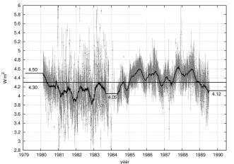
Figure 4: Relative difference between NIMBUS7/ERB and SMM/ACRIM1 TSI records.

The data shown in Figure 4 have an average of $4.3W/m^{2}$. The original ACRIM TSI composite [Willson and Mordvinov, 2003] is constructed in a way which is equivalent to use the above average value to merge SMM/ACRIM1 and NIMBUS7/ERB record.

However, if the differences between SMM/ACRIM1 and the NIMBUS7/ERB records were only due to random fluctuations around an average value, the error associated to the 91-day moving average values had to be about $\pm 0.02$-$0.03W/m^{2}$, as calculated from the measurement uncertainties. Because the standard deviation of the smooth data shown in Figure 4 is significantly larger, $\pm 0.17W/m^{2}$, the difference between SMM/ACRIM1 and NIMBUS7/ERB measurements is not just due to random fluctuations, but due to biases and trends in the data probably due to poor sensor calibration of NIMBUS7/ERB.

Under the theoretical assumption that the SMM/ACRIM1 measurements are more accurate than NIMBUS7/ERB, the black 91-days moving average smooth curve shown in Figure 4 suggests that NIMBUS7/ERB measurements could gradually shift during a relatively short period of time, a few months, by an amount that on average is about $0.2W/m^{2}$, and in a few cases can also be as large as $0.5W/m^{2}$. In fact, irregular large oscillations with periods ranging from 5 to 12 months are clearly visible in Figure 4.

The above finding shows that the original methodology adopted by the ACRIM team to merge SMM/ACRIM1 and NIMBUS7/ERB records is likely inappropriate because it assumes that NIMBUS7/ERB data are statistically stationary, that is, unbiased, while this is not what is found in the data. By not taking into account this problem the ACRIM team’s methodology can introduce significant artificial slips in the TSI satellite composite at the chosen merging day.

To reduce the errors due to the above irregular large oscillations of NIMBUS7/ERB measurements we used the black 91-days moving average smooth curve shown in Figure 4 to reduce NIMBUS7/ERB record to the level of SMM/ACRIM1 during the overlapping period and, thus, use the NIMBUS7/ERB corrected record to fill all days SMM/ACRIM1 record misses. Before 17/02/1980 NIMBUS7/ERB record is shifted by $-4.5W/m^{2}$, while after 14/07/1989 it is shifted by $-4.12W/m^{2}$. This means that relative to the original ACRIM composite, our composite will be $0.2W/m^{2}$ lower before 17/02/1980, and $0.18W/m^{2}$ higher after 14/07/1989.

However, these values do depend on the moving average window adopted. In fact, by increasing the window the two above levels will approach to the average level at $-4.3W/m^{2}$, which is the value used by the ACRIM team to merge the two records. Thus, the above two estimates can have an error as large as $0.2W/m^{2}$.

On the contrary, the PMOD team significantly alters both SMM/ACRIM1 and NIMBUS7/ERB records before 1986: see Figure 3. These corrections are not justified by the data themselves, but by theoretical models, which can be erroneous and/or may have large uncertainties. About the SMM/ACRIM1 data PMOD team assumes that the SMM/ACRIM1 record from 1984 to 1986 significantly degradated: as Figure 3 shows, the position of NIMBUS7/ERB relative to SMM/ACRIM1 gradually increases from 1984 to 1986. However, this pattern can be caused both by a degradation of SMM/ACRIM1, as the PMOD team interprets, and by an increase of sensitivity of NIMBUS7/ERB sensors due to undetermined factors. In fact, we observe that from 1988 to 1989.5 the position of NIMBUS7/ERB relative to SMM/ACRIM1 gradually decreased of the same amount of the gradual increase observed from 1984 to 1986. This suggests that NIMBUS7/ERB record of the TSI can gradually vary by these large amounts.

In any case, ACRIM team has never published an update of their SMM/ACRIM1 record and publicly disagreed with the PMOD team on many occasions on this issue [Willson and Mordvinov, 2003] because they were not able to find any physical explanation for this presumed degradation of the SMM/ACRIM1 record. Herein, we believe that the ACRIM team opinion cannot be just ignored and dismissed given the fact they are the authors of the data. The correction implemented by the PMOD team on the SMM/ACRIM1 record should be considered hypothetical and not taken as granted. In any case, this correction would not alter the position of the TSI minimum in 1985/1986 relative to the minimum in 1996, which herein is a more important issue; PMOD team’s correction would only lower the TSI maximum in 1981/1982 by about $0.2W/m^{2}$ relative to the TSI satellite composite after 1986.

About the NIMBUS7/ERB record before 1980, although NIMBUS7/ERB trends appear to be quite uncertain, the PMOD team’s correction of them should be considered hypothetical as well because they are not justified by other satellite measurements. In particular, PMOD team believes that the large NIMBUS7/ERB peak occurred during the first months of 1979 (see Figures 1 and 2) is an artifact due to changes in the orientation of the spacecraft that has to be corrected. However, we observe that TSI theoretical reconstruction proposed by Solanki [Wenzler et al., 2006] shows that a large TSI peak occurred during the first months of 1979. Look carefully at their figures 14 and 15 where the TSI proxy reconstruction is compared with the PMOD composite; during the first months of 1979 there is a discrepancy of about $1W/m^{2}$ between the two records. This is a sufficient evidence for considering the PMOD team’s corrections of NIMBUS7/ERB suspicious.

In any case, the exact TSI patterns before 17/02/1980 and during the ACRIM-gap should be considered highly uncertain because they have to be derived from low quality satellite measurements.

3 The ACRIM-gap: 15/07/1989 - 03/10/1991

SMM/ACRIM1 and UARS/ACRIM2 records can only be bridged by using two low quality satellite records: NIMBUS7/ERB and ERBS/ERBE. Figure 5 shows the two records. Note that NIMBUS7/ERB and ERBS/ERBE present opposite trend. From 1990 to 1991.5 NIMBUS7/ERB record shows an increasing trend while ERBS/ERBE record shows a decreasing trend [Willson and Mordvinov, 2003]. Thus, the only two available satellite records are not compatible with each other and at least one of the two is corrupted. Note that ERBS/ERBE too was unable to calibrate its sensor degradations and a direct comparison with the ACRIM records reveals that the discrepancy between local ACRIM smooth trends and the ERBS/ERBE smoth trends may as large as $\pm 0.2W/m^{2}$: the amplitude of these non-stationary biases is smaller than that observed in the NIMBUS7/ERB measurements, but they are still significant. Moreover, the average error of ERBS/ERBE’s measurements are the largest among all satellite observations: $\pm 0.26W/m^{2}$.

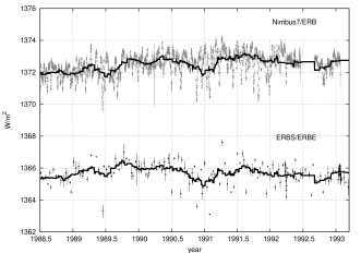
Figure 5: NIMBUS7/ERB and ERBS/ERBE TSI records during the ACRIM-gap. The smooth curves are 91-day moving averages calculated on the TSI values only for those days available in both records.

The PMOD team claims that NIMBUS7/ERB record must be severely corrected during the ACRIM-gap. The reasons of these corrections can be found in the literature. Lee III et al. [1995] compared the NIMBUS7/ERB dataset with a TSI proxy model based on a multi-regression analysis of March 1985 to August 1989 ERBS/ERBE irradiance measurements. They concluded that after September 1989 NIMBUS7/ERB time series appeared to abruptly increase by $+0.4W/m^{2}$ after a switch-off of NIMBUS7/ERB for four days. Another $+0.4W/m^{2}$ upward shift appeared to occur on April 1990. Thus, this model suggests a two step shift correction that, once combined, would require the NIMBUS7/ERB record to be shifted down by $0.8W/m^{2}$ at the end of April 1990.

Later Chapman et al. [1996] review the finding by Lee et al. [1995] and concluded that on 29/09/1989 there was an upward shift of $+0.31W/m^{2}$ and on 9/05/1990 there was an upward shift of $+0.37W/m^{2}$: the new proposed combined two step correction shift had to be -0.68 $W/m^{2}$ after 9/05/1990. Afterward, Fröhlich and Lean [1998] suggested a different two step shift correction, that is, the NIMBUS7/ERB record had to be adjusted by $-0.26W/m^{2}$ and $-0.32W/m^{2}$ near October 1, 1989, and May 8, 1990, respectively. According the latter model during the ACRIM-gap NIMBUS7/ERB had to be shifted down by 0.58 $W/m^{2}$.

Finally, Fröhlich [2004, 2006] revised significantly his previous model correction of NIMBUS7/ERB data. He first acknowledged that the supposed slip on May 1990 was indeed difficult to really identify. Then, he substituted the two step correction model with a new model in which there was only one slip on 29 September 1989 followed by a upward linear trend. Figure 6 shows our analysis of these new corrections in their latest version: on 29/09/1989 there is a supposed slip of $+0.47W/m^{2}$, which is significantly larger than what was previously estimated, the upward trend is $+0.142Wm^{-2}/year$. The total downward shift forced on NIMBUS7/ERB record from 1989.5 to 1992.5 is about $0.86W/m^{2}$, which is significantly larger than what was previously estimated by Fröhlich himself and the other groups.

Figure 6: Relative difference between NIMBUS7/ERB original record and PMOD TSI satellite composite.

From the above studies it is evident that several opinions have been formulated to solve the ACRIM-gap, even by the same research team, and they quantitatively disagree with each other. The above conflicting solutions indicate that it is not so certain how NIMBUS7/ERB should be corrected, if some corrections are truly needed.

Figure 7 shows our analysis of the comparison between NIMBUS7/ERB and ERBS/ERBE. The 91-day moving average curve of the relative difference between NIMBUS7/ERB and ERBS/ERBE decreases until August 1989 around the time when SMM/ACRIM1 merges with NIMBUS7/ERB at the level $6.29W/m^{2}$, as shown in the graph. Since the beginning of September 1989 to the beginning of 1990 the curve rises rapidly by about $0.65W/m^{2}$. From 1990 to 1991.5 the curve rises by about $0.40W/m^{2}$. Finally, from 1991.5 to 1993 the curve decreases slightly by about $0.05W/m^{2}$.

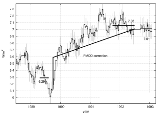
Figure 7: 91-day moving average of the relative difference between NIMBUS7/ERB original record and ERBS/ERBE TSI satellite composite during the ACRIM-gap. The figure shows the correction of NIMBUS7/ERB record implemented by PMOD team shown in Figure 6(solid line).

The total shift from 1989.5 to 1993 is about $0.72W/m^{2}$. Note that the error related to the single measurements is about $\pm 0.11W/m^{2}$. Thus, the observed difference between NIMBUS7/ERB and ERBS/ERBE is significant and must be interpreted as due to biases in the data that are due to uncorrected degradation problems in the sensors or something else that biases the TSI record.

Figure 7 shows also the correction implemented by the PMOD team on NIMBUS/ERB record [Froöhlich 2004, 2006]. It is evident that the PMOD team believes that the observed difference is due to uncorrected problems occurring only on NIMBUS7/ERB’s sensors. Even so, the correction of NIMBUS/ERB record implemented by the PMOD team ( $0.86W/m^{2}$ from 1989.5 to 1992.5) appears to be overestimated at least by about $0.09W/m^{2}$ because the total shift observed during the period is no more than about $0.77W/m^{2}$. The difference seems to be due to the fact that PMOD team did not take into account that the real comparison must be done with the level when SMM/ACRIM1 merges with NIMBUS7/ERB around the middle of 1989, and the level during this period, as indicated in the figure, is about $6.29W/m^{2}$. Thus, if on 29/09/1989 a jump really occurred in the NIMBUS7/ERB record, this has to be about $0.30W/m^{2}$, as previously estimated by Chapman et al. [1996] and Froöhlich and Lean [1998]. Finally, the PMOD team’s correction with a linear increase from 29/09/1989 to 1992.5 is poorly observed in data shown in Figure 7; it appears to be just a linear simplification of the complex pattern observed in the figure.

The major problem with the interpretation of the theoretical studies [Lee III et al., 1995; Chapman et al., 1996; Froöhlich and Lean, 1998; Froöhlich, 2004, 2006] claiming that NIMBUS7/ERB is erroneous during the ACRIM-gap is that, although these authors did notice a difference between NIMBUS7/ERB and ERBS/ERBE records, they have interpreted such a difference as only due to a corruption of the NIMBUS7/ERB record despite the fact that ERBS/ERBE too was unable to continuously calibrate its sensor degradations and its data had larger uncertainties than NIMBUS7/ERB data. Indeed, the increase observed in Figure 7 during the ACRIM gap could result from increased ERBS/ERBE degradation relative to NIMBUS7/ERB, a relative increase in the sensitivity of the NIMBUS7/ERB sensor, or both [Willson, 1997].

It is important to stress that in 1992 the experimental team responsible of NIMBUS7/ERB record [Hoyt et al., 1992] corrected all biases in the data they could find and after that ever come up with a physical theory for the instrument that could cause it to become more sensitive. The NIMBUS7/ERB calibrations before and after the September 1989 shutdown gave no indication of any change in the sensitivity of the radiometer. When Lee III et al. of the ERBS team claimed there was an increase in NIMBUS7/ERB sensitivity, the NIMBUS7 team examined the issue and concluded there was no internal evidence in the NIMBUS7/ERB record to warrant the correction that the latter team was proposing (personal communication with Hoyt in Scafetta and Willson [2009]). Perhaps the increase between 1989 and 1991 in Figure 7 is indications of ERBS losing sensitivity rather than NIMBUS7 gaining sensitivity.

There are several physical reasons to believe that ERBS/ERBE could degrade more likely than NIMBUS7/ERB in particular during the ACRIM-gap. For example: a) The NIMBUS7/ERB cavity radiometer was in a relatively high altitude (about 900 km) while ERBS/ERBE was in a low earth orbit (ca. 200 km). It is possible that ERBS would degrade much faster than NIMBUS7/ERB due to more atmospheric bombardment of its sensor. b) During the ACRIM-gap ERBS/ERBE was experiencing for the first time the enhanced solar UV radiation, which occurs during solar maxima, and this too may have caused a much faster degradation of the cavity coating of ERBS than of NIMBUS7/ERB because NIMBUS7 already experienced such degradation during the previous solar maximum; c) From the spring 1990 to May/June 1991, when according to Figure 7 the difference between NIMBUS7/ERB and ERBS/ERBE increased by about $0.40W/m^{2}$, there was a rapid increase of cosmic ray flux, as Figure 8 shows. Also the latter phenomenon might have more likely affected ERBS/ERBE’s sensors than NIMBUS7/ERB’s ones, which already experienced a solar maximum 10 years earlier.

Moreover, the cosmic ray count is negative-correlated to TSI and magnetic flux, thus its minima correspond to solar activity maxima. Figure 8 shows that the minimum around 1991.5 was lower than the minimum around 1989.8-1990.5. This implies that according to this record the solar activity was likely higher around 1991.5 than around 1989.8-1990.5. This contradicts the pattern observed in ERBS/ERBE while confirming NIMBUS7/ERB pattern, as Figure 5 shows. However, other solar indexes, such as the sunspot number index, present the opposite scenario. Thus, it is unlikely that solar proxies indexes can be used to solve this issue definitely.

Figure 8: Climax cosmic ray of the University of New Hampshire (Version 4.8 21 December 2006). Data from http://ulysses.sr.unh.edu/NeutronMonitor/.

Thus, unless the experimental teams find a physical theory for explaining the divergencies observed in their own instrumental measurements and solve definitely the problem, there exists only a statistical way to address the ACRIM-gap problem by using the published data themselves. This requires just the acknowledgment of the existence of an unresolved uncertainty in the TSI satellite data. This can be done by:

1) Assuming that NIMBUS7/ERB is correct and ERBS/ERBE is erroneous; this would imply that during the ACRIM-gap ERBS/ERBE record degraded and should be shifted upward by $0.72$-$0.77W/m^{2}$.

2) Assuming that ERBS/ERBE is correct and NIMBUS7/ERB is erroneous; this would imply that during the the ACRIM-gap NIMBUS7/ERB increased its sensitivity to TSI and should be shifted downward by $0.72$-$0.77W/m^{2}$.

3) Assuming that both ERBS/ERBE and NIMBUS7/ERB records need some corrections.

Note that there is no objective way to implement method n. 3 and infinitely different solutions may be proposed. For example, the one proposed by the PMOD team is just one proposal among many others. Herein we propose that all configurations between case n. 1 and case n. 2 may by possible, and for case n. 3 we just propose an average between the methods 1 and 2 stressing that this arithmetic average should not be interpreted as a better physical solution to the ACRIM-gap problem.

Figure 9 shows the three reconstructions of NIMBUS7/ERB record in agreement with the above three scenarios: [A] NIMBUS7/ERB data are unaltered; [C] the NIMBUS7/ERB data are altered in such a way that their 91-day moving average curve in Figure 9 matches exactly the 91-day moving average curve of ERBS/ERBE shown in Figure 5; finally, in [B] the NIMBUS7/ERB data are altered in such a way that their 91-day moving average curve matches exactly the average between the two 91-day moving average curves of NIMBUS7/ERB and ERBS/ERBE shown in Figure 5.

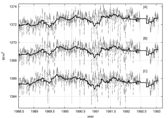
Figure 9: Reconstructions of the NIMBUS7/ERB record during the ACRIM-gap in agreement with three alternative scenarios. [A] data are unaltered; [C] the data are adapted in such a way that their smooth component matches exactly the smooth component of ERBS/ERBE; [B] the data are adapted in such a way that their smooth component matches exactly the average between the smooth components in [A] and [C].

4 SMM/ACRIM1 vs. UARS/ACRIM2

To align SMM/ACRIM1 and UARS/ACRIM2 records we proceed as follows. First, we merge NIMBUS7/ERB record and its two alternative records shown in Figure 9 with the SMM/ACRIM1 record. The merging is done by uniting the 91-moving average mean curves at the merging day, 03/10/1991.

Second, we use the finding shown in Figure 10. This figure shows the overlapping period between NIMBUS7/ERB and UARS/ACRIM2 records. This interval is quite short and is made of two separated intervals during which both satellite measurements were interrupted for several months. Note that the two intervals are not aligned: there is a difference of about $0.2W/m^{2}$ between the two levels. Because the standard deviation of the data is about $0.26W/m^{2}$ which is significantly larger than the statistical error of measure $0.16W/m^{2}$, the figure indicates that the data are not statistically stationary.

Figure 10: Relative difference between NIMBUS7/ERB and UARS/ACRIM2 TSI satellite records according to the three hypotheses discussed in the article. Note that NIMBUS7/ERB record has been already merged with SMM/ACRIM1 record. Thus, the value reported in the figure refers to the position SMM/ACRIM1 relative to UARS/ACRIM2 in the three alternative cases.

However, it is not evident which is performing poorly: NIMBUS7/ERB and ERBS/ERBE or UARS/ACRIM2. Because the difference observed between NIMBUS7/ERB and UARS/ACRIM2 records in [A], and between the adapted NIMBUS7/ERB and UARS/ACRIM2 records in [C] (where NIMBUS7/ERB record is adapted to reproduce the smooth of the ERBS/ERBE record) are almost equal, the first impression is that UARS/ACRIM2 sensors experienced a downward slip between the two intervals by about $0.2W/m^{2}$. However, because both NIMBUS7/ERB and ERBS/ERBE were less able to calibrate their sensor degradation, it is still uncertain whether it is UARS/ACRIM2 record that has to be corrected and, if so, how large this corrections should be. Indeed, given the short time period and that both NIMBUS7/ERB and ERBS/ERBE are characterized by non stationary biases as large as $\pm 0.2W/m^{2}$, it is possible that during 1992 the two latter records experienced a similar upward bias. Thus, here we decided to keep UARS/ACRIM2 record unaltered and merge the two sequences using the average of the relative differences during the entire overlapping period in all three cases, as shown in the Figure 10. The error associated with this merging is about $\pm 0.1W/m^{2}$. However, if UARS/ACRIM2 record does need to be corrected, the global implication of this correction would be that the TSI satellite composite before 1992.5 should be shifted downward by about $0.1W/m^{2}$ in all three cases.

5 UARS/ACRIM2 vs. ACRIMSAT/ACRIM3

The merging between UARS/ACRIM2 and ACRIMSAT/ACRIM3 is done by using the information shown in Figure 11 that shows the relative difference between ACRIMSAT/ACRIM3 and UARS/ACRIM2, and for comparison, the relative difference between SOHO/VIRGO and UARS/ACRIM2. Note that the UARS/ACRIM2 measurements were interrupted from 05/06/2001 to 08/16/2001.

Figure 11: Relative difference between ACRIMSAT/ACRIM3 and UARS/ACRIM2 TSI satellite records (Top) and between SOHO/VIRGO and ACRIM2 TSI satellite records (Bottom). The latter is shifted down by $1W/m^{2}$ for visual clarity.

The latter comparison is necessary for determining the reason of the discrepancy observed between ACRIMSAT/ACRIM3 and UARS/ACRIM2 which is significantly larger than the statistical error associated with the measurements. In fact, the average statistical error of UARS/ACRIM2 data is $0.01W/m^{2}$, while the average statistical error of ACRIMSAT/ACRIM3 data is $0.008W/m^{2}$. The average statistical error of the relative difference between ACRIMSAT/ACRIM3 and UARS/ACRIM2 is no more than $0.018W/m^{2}$. However, the data in the figure have a standard deviation of about $0.3W/m^{2}$ which is significantly larger than the statistical errors. Thus, the observed difference between ACRIMSAT/ACRIM3 and UARS/ACRIM2 records is not due to random fluctuations, but to non-stationary trends in the data.

Because a similar pattern appears when UARS/ACRIM2 is compared with both SOHO/VIRGO and ACRIMSAT/ACRIM3 records, it is likely that UARS/ACRIM2 sensors may have been experiencing some problem. Perhaps the annual cycle has been filtered off in some way. However, these problems appear to have significantly modified a natural variation in the TSI data characterized by a time scale close to 1 year. Because the difference between ACRIMSAT/ACRIM3 and UARS/ACRIM2 appears to present a cyclical pattern, an accurate way to merge the two sequences is to evaluate the average during an entire period of oscillation. The period from 04/05/2000 to 05/06/2001 covers approximately one period of oscillation, and during this period the average difference between ACRIMSAT/ACRIM3 and UARS/ACRIM2 is $1.86W/m^{2}$: we use this value for the merging. As the figure shows the averages during the first and the second half of the cycle are $1.70W/m^{2}$ and $2.02W/m^{2}$, respectively. This suggests that our merging has an uncertainty of about $\pm 0.18W/m^{2}$.

6 Three updated ACRIM TSI composites

The satellites records are merged and our three TSI composites are shown in Figure 12. Table 1 summarizes how SMM/ACRIM1 and UARS/ACRIM2 records have to be adjusted to be aligned with ACRIMSAT/ACRIM3.

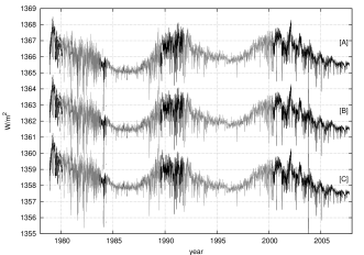
Figure 12: The three TSI satellite conposites. The composites [B] and [C] are shifted by $-4W/m^{2}$ and $-8W/m^{2}$, respectively, for visual clarity.

The composite [A] shows that the 1996 minimum is about $0.67\pm 0.1W/m^{2}$ higher than the 1986 minimum. The composite [B] shows that the 1996 minimum is about $0.28\pm 0.1W/m^{2}$ higher than the minimum in 1986. The composite [C] shows that the 1996 minimum is about $0.11\pm 0.1W/m^{2}$ lower than the minimum in 1986. Thus, only in the eventuality that during the ACRIM-gap ERBS/ERBE data are uncorrupted the two solar minima would almost coincide, while on average the data indicate that the TSI minimum in 1996 is $0.28\pm 0.4W/m^{2}$ higher than the minimum in 1985/6.

Note that if UARS/ACRIM2 record needs to be corrected during its superposition with NIMBUS7/ERB, as explained above, the TSI 1996 minimum relative to the TSI 1986 minimum would be about $0.1W/m^{2}$ higher than the above three estimates. Thus, if this is the case, according to the satellites data the difference between the two minima would be about $0.38\pm 0.4W/m^{2}$. This would further stress that the TSI satellite data do indicate that TSI likely increased during solar cycles 21-23 (1980-2002).

	[A]	[B]	[C]
A1	$-1.90\pm 0.19$	$-1.51\pm 0.19$	$-1.12\pm 0.19$
A2	$+1.86\pm 0.16$	$+1.86\pm 0.16$	$+1.86\pm 0.16$
A3	$0$	$0$	$0$

Table 1: Position in $W/m^{2}$ of SMM/ACRIM1 (A1) and UARS/ACRIM2 (A2) relative to ACRIMSAT/ACRIM3 (A3) in the three scenarios [A], [B] and [C] as discussed in the test. The errors are calculated by taking into account the highest uncertainty due to the statistical non-stationarity of NIMBUS7/ERB and UARS/ACRIM2 when they merge and when UARS/ACRIM2 merges ACRIMSAT/ACRIM3. Note that the error of the position of SMM/ACRIM1 compared to UARS/ACRIM2 is $\pm 0.1W/m^{2}$. The error associated to the non-stationarity of NIMBUS7/ERB during the ACRIM-gap is described by the three scenarios [A], [B] and [C].

7 TSI proxy secular reconstructions

It is necessary to use reconstructions of the solar activity as long as possible, at least one century, for determining the effect of solar variations on climate. The TSI record that is possible to obtain from direct TSI satellite measurements covers the period since 1978, and this period is far too short to correctly estimate how the Sun may have altered climate. The reason is because the climate system is characterized by a slow characteristic time response to external forcing that is estimated to be about 8 years (which, theoretically, can be as large as 12 years) [Scafetta, 2008; Schwartz, 2008]. This decadal time response of the climate requires several decade long records for a correct evaluation of an external forcing on climate. Thus, it is necessary to merge the TSI satellite composites with the long TSI secular reconstructions, which are quite uncertain because they are necessarily based on proxy data, and not direct TSI measurements.

Long-term TSI changes over the past 400 years since the 17th-century Maunder minimum have been reconstructed by several authors, for example: Hoyt and Schatten [1997], Lean [2000], Wang et al. [2005] and Krivova et al. [2007]. These TSI proxy reconstructions are based on the sunspot number record, the long-term trend in geomagnetic activity, the solar modulation of cosmogenic isotopes such as ${}^{14}C$ and ${}^{10}Be$ records, and other solar related records. These observables are used because they are supposed to be linked to TSI variations. However, it is not known exactly how the TSI can be reconstructed from these historical records nor whether these records are sufficient to faithfully reconstruct TSI changes. Thus, the proposed TSI secular proxy reconstructions are quite different from each other and show different patterns, trends and maxima, as depicted in Figure 13. Nevertheless, they reproduce similar patterns: in particular, note the minima during the Maunder Minimum (1645-1715) and the Dalton Minimum (1790-1820), and the TSI increase during the first half of the 20^th century.

Figure 13: Secular TSI proxy reconstructions by Hoyt and Schatten [1997] (HS1997), Lean [2000] (L2000), Wang et al. [2005] (W2005) and Krivova et al. [2007] (K2007). K2007 has been shifted by $-3W/m^{2}$ for visual convenience.

The TSI increase during the first half of the 20^th century is particularly important. In fact, because the characteristic time response of climate to external forcing is about 8-12 years, an increase of TSI during the first half of the 20^th century would induce a warming also during the second half of the 20^th century, even if the TSI remains almost constant during the second half of the 20^th century [Scafetta and West, 2007].

The four TSI proxy reconstructions shown in Figure 13 present different trends since 1975. The TSI reconstruction by Hoyt and Schatten [1997] suggests that TSI increased during this period, as shown in our TSI satellite composites [A] and [B], and in the original ACRIM TSI satellite composite. However, the other three TSI proxy reconstructions [Lean, 2000; Wang et al., 2005; Krivova et al., 2007] suggest that TSI did not change on average since 1978, as shown in our TSI satellite composite [C] and in the PMOD TSI satellite composite. Thus, the uncertainty that we have found in composing the TSI satellite records appears unresolved also by using the TSI proxy reconstructions because different solar proxies do suggest different TSI patterns as well.

Because the TSI satellite composites refer to the actual TSI measurements, we propose their merging with the TSI proxy reconstructions for obtaining a TSI secular record. Here, we chose the most recent TSI proxy reconstruction [Krivova et al., 2007], which has a daily resolution, and merge it to the TSI satellite composites in such a way that their 1980-1990 average coincides. Other choices and their implications by using the original ACRIM and the PMOD TSI satellite composites with the TSI proxy reconstructions of Lean [2000] and Wang et al. [2005] can be found in Scafetta and West [2007]. The three TSI merged records herein proposed are shown in Figure 14. The figure shows that during the last decades the TSI has been at its highest values since the 17^th century.

Figure 14: Merging of the secular TSI proxy reconstruction by Krivova et al. [2007] (black) with the three TSI satellite composites proposed in Figure 12 (grey). The TSI reconstructions [B] and [C] are shifted by $-5W/m^{2}$ and $-10W/m^{2}$, respectively, for visual convenience. The merging is made by shifting the original secular TSI proxy reconstruction by Krivova et al. [2007] by $-0.5174W/m^{2}$, $-0.1295W/m^{2}$ and $+0.2584W/m^{2}$ in the case [A], [B] and [C] respectively.

8 Phenomenological solar signature on climate

The phenomenological solar signature on climate can be estimated with a phenomenological energy balance model (PEBM) [Scafetta and West, 2007]. PEBM assumes that the climate system, to the lowest-order approximation, responds to an external radiative forcing as a simple thermodynamical system, which is characterized by a given relaxation time response $\tau$ with a sensitivity $\alpha$. The physical meaning of it is that a small anomaly (with respect to the TSI average value) of the solar input, measured by $\Delta I$, forces the climate to reach a new thermodynamic equilibrium at the asymptotic temperature value $\alpha\Delta I$ (with respect to a given temperature average value). Thus, if $\Delta I(t)$ is a small variation (with respect to a fixed average) of an external forcing and $\Delta T_{s}(t)$ is the Earth’s average temperature anomaly induced by $\Delta I(t)$, $\Delta T_{s}(t)$ evolves in time as:

$$\frac{d\Delta T_{s}(t)}{dt}=\frac{\alpha\Delta I(t)-\Delta T_{s}(t)}{\tau}.$$ (1)

A model equivalent to (1) has been used as a basic energy balance model [North et al., 1981; Douglass and Knox, 2005], but herein we use TSI records as a proxy forcing.

We implement the PEBM by imposing that the global peak-to-trough amplitude of the 11-year solar cycle signature on the surface temperature is about $0.1K$ from 1980 to 2002, as found by several authors (see IPCC [2007], page 674 for details). This implies that the climate sensitivity $Z_{11}$ to the 11-year solar cycle is

$$Z_{11}=0.11\pm 0.02K/Wm^{-2},$$ (2)

as found by Douglass and Clader [2002], and Scafetta and West [2005]. In addition the characteristic time response to external forcing has been phenomenologically estimated to be $\tau=8\pm 2$ years [Scafetta, 2008; Schwartz, 2008]. Note that Scafetta [2008] has also found that climate is characterized by two characteristic time constants $\tau_{1}=0.40\pm 0.1$ and $\tau_{2}=8\pm 2$, with the latter estimate that may be a lower limit (the upper limit being $\tau_{2}=12\pm 3$ years), but a discussion about the consequences of this finding is left to another study [Scafetta, 2009].

The value of the parameter $\alpha$ is not calculated theoretically by using the TSI as a climate forcing as usually done in the traditional climate models. The value of $\alpha$ is calculated by using the phenomenological climate sensitivity to the 11-year solar cycle found in Eq. [2] by means of the following equation

$$\alpha(\tau)=Z_{11}\sqrt{1+\left(\frac{2\pi\tau}{11}\right)^{2}},$$ (3)

which solves Eq. [1]. Thus, we find that the phenomenological climate sensitivity to TSI changes is

$$\alpha=0.51\pm 0.15K/Wm^{-2}.$$ (4)

With the above value of $\tau$ and $\alpha$ Eq. [1] can be numerically solved by using as input the TSI records shown in Figure 14. The phenomenological solar signatures (PSSs) are shown in Figure 15 where the three PSSs are plotted since 1600 against a paleoclimate Northern Hemisphere temperature reconstruction [Moberg et al., 2005] and since 1850 against the actual instrumental Northern Hemisphere surface record [Brohan et al., 2006].

The figure shows that there is a good agreement between the PSSs and the temperature record. The patterns between 1600 and 1900 are well recovered. The warming during the first half of the 20^th century is partially recovered. Finally, since 1978 the output strongly depends on the TSI behavior. If the TSI reconstruction [A] is adopted, a significant portion of the warming, about 66% observed since 70s has been induced by solar variations, while if the TSI reconstruction [C] is adopted, almost all warming, about 85% observed since 70s has been induced by factors alternative to solar variations. If the average TSI reconstruction [B] is adopted, at most 50% of the warming observed since 70s has been induced by solar variations.

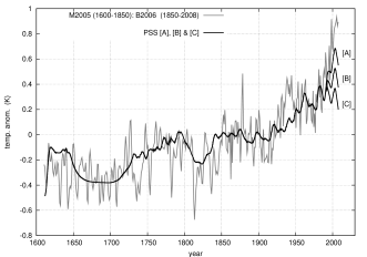
Figure 15: The three phenomenological solar signatures on climate (black) obtained with Eq. 1 forced with the three TSI records shown in Figure 14 against a paleoclimate Northern Hemisphere temperature reconstruction [Moberg et al., 2005] from 1600 to 1850, and since 1850 against the actual instrumental Northern Hemisphere surface record [Brohan et al., 2006] (grey). The figure shows temperature anomalies relative to the 1895-1905 average.

9 Conclusion

We have reconstructed new TSI satellite composites by using the three ACRIM records. We have shown that different composites are possible depending on how the ACRIM-gap from 1989.5 to 1992 is solved. Our three TSI composites indicate that the TSI minimum in 1996 is at least approximately $0.30\pm 0.40W/m^{2}$ higher than the TSI minimum in 1986. And that the two minima would approximately be located at the same level only in the eventuality that the TSI ERBS/ERBE satellite record is uncorrupted during the ACRIM-gap, a fact that may be not likely.

None of the TSI satellite composites proposed by the ACRIM, IRMB and PMOD teams can be considered rigorously correct. All three teams have just adopted alternative methodologies that yield to different TSI composites, but these teams have ignored the unresolved uncertainty in the data that yields to an unresolved uncertainty in the TSI composites as well.

Note that comparison with theoretical TSI proxy models, for example Wenzler et al., [2006] and Krivova et al. [2007], cannot be used to resolve the issue, as the PMOD team assumes, because: 1) In science theoretical models have to be tested against the observations, not vice versa; 2) The TSI proxy models adopt a reductionistic scientific approach, that is, they assume that some given solar observable that refers to a particular solar measure (for example measurements from magnetograms or measurements of the intensity of a given frequency of the spectrum) can be used to faithfully reconstruct a global solar measure such as the TSI; 3) The TSI proxy models do depend on parameters that opportunely calibrated give different outcomes that can, eventually, fit alternative satellite composites.

Thus, because it is not possible to reconstruct with certainty the TSI behavior during the ACRIM-gap, the TSI decadal trend during the last three decades is unfortunately uncertain, and any discussion that needs to use the TSI record has to take into account this unresolved uncertainty.

However, because the uncertainty in the data indicate that the TSI minimum in 1996 is at least approximately $0.30\pm 0.40W/m^{2}$ higher than the TSI minimum in 1986, on average the satellite records do suggest that TSI may have increased from 1980 to 2000. Therefore, the sun may have significantly contributed to the warming observed during the last three decades, as suggested by the phenomenological energy balance model simulations herein proposed.

Note that a recent paper by Lockwood [2008] concludes that even with the adoption of the original ACRIM composite, the sun’s contribution to the global surface warming would be negligible during the last three decades, in contrast with the findings of Scafetta and West [2007,2008] and those presented here. However, Lockwood’s findings derive from his evaluation of the characteristic time response of the climate to solar variation: $\tau=0.8$ years. This value strongly differs from the value herein adopted of $\tau=8$ years and recently measured by Scafetta [2008] and Schwartz [2008]. The problem with Lockwood’s short time constant is that according to the climate physics implemented in most climate models, the characteristic time response of the climate varies from a few months to several years and even decades, as Lockwood himself acknowledges in his paper (see references there). For example, the linear upwelling/diffusion energy balance model used by Crowley [2000] is characterized by a time response of about $\tau=10$ years. In addition, Scafetta [2008] and Schwartz [2008] have found that climate is indeed characterized by two characteristic time constants, one short with a time scale of several months and one long with a decadal time scale. The climate processes with a fast response are usually responsible for the fast fluctuations seen in the data. Instead, the climate processes with a slow response are those that drive the decadal and secular trends observed in the global temperature. This slow climate response derives from the fact that the processes that regulate the decadal and secular variation of climate (most of all energy exchange with the deep ocean and changes of the albedo due to the melting of the glaciers and forestation and desertification processes) are very slow processes, and they work as powerful climate feedbacks. Thus, we believe that Lockwood’s analysis is inappropriate because it failed to take into account the climate processes with a slow time response that would be responsible of a strong climate response to solar changes. However, a more detailed discussion about this issue, which would imply also an update of the PEBM presented here, is left to another study [Scafetta, 2009].

Acknowledgment: NS thanks the Army Research Office for research support (grant W911NF-06-1-0323).

References

- [1] Brohan P., J. J. Kennedy, I. Harris, S. F. B. Tett and P. D. Jones, 2006, Uncertainty estimates in regional and global observed temperature changes: A new dataset from 1850, Journal of Geophysical Research, v. 111, D12106. (doi:10.1029/2005JD006548)
- [2] Chapman G. A., A. M. Cookson and J. J. Dobias, 1996, Variations in total solar irradiance during solar cycle 22, Journal of Geophysical Research, v. 101, p. 13541 13548. (doi:10.1029/96JA00683)
- [3] Crommelynck D. and S. Dewitte, 1997, Solar constant temporal and frequency characteristics, Solar Physics, v. 173, p. 177 191.
- [4] Crowley T. J., 2000, Causes of Climate Change Over the Past 1000 Years, Science v. 289, p. 270-277.
- [5] Douglass, D. H., and B. D. Clader (2002), Climate sensitivity of the Earth to solar irradiance, Geophys. Res. Lett., v. 29. (doi: 10.1029/2002GL015345).
- [6] Douglass, D. H., and R. S. Knox, 2005, Climate forcing by the volcanic eruption of Mount Pinatubo, Geophysical Research Letters, v. 32, L05710. (doi:10.1029/2004GL022119)
- [7] Dewitte S., D. Crommelynck, S. Mekaoui, A. Joukoff, 2004, Measurement and uncertainty of the long-term total solar irradiance trend, Solar Physics, v. 224, p. 209 216. (doi:10.1007/s11207-005- 5698-7)
- [8] Fröhlich, C., D. Crommelynck, C. Wehrli, M. Anklin, S. Dewitte, A. Fichot, W. Finsterle, A. Jimènez, A. Chevalier and H. J. Roth, 1997, In-flight performances of VIRGO solar irradiance instruments on SOHO, Solar Physics, v. 175, p. 267 286.
- [9] Fröhlich C. and J. Lean, 1998, The Sun s total irradiance: cycles, trends and related climate change uncertainties since 1978, Geophysical Research Letters, v. 25, p. 4377 4380. (doi:10.1029/1998GL900157).
- [10] Fröhlich C., 2000, Observations of irradiance variations, Space Science Reviews, v. 94, p. 15 24. (doi:10.1023/A:1026765712084).
- [11] Fröhlich C., 2004, Solar irradiance variability: In Geophysical Monograph 141: Solar Variability and its Effect on Climate, American Geophysical Union, Washington DC, USA, Chapt. 2: Solar Energy Flux Variations, p. 97 110.
- [12] Fröhlich C., 2006, Solar irradiance variability since 1978: revision of the PMOD composite during solar cycle 21: Space Science Reviews, v. 125, p. 53 65. (doi:10.1007/s11214-006-9046-5)
- [13] Hoyt D. V., H. L. Kyle, J. R. Hickey, and R. H. Maschhoff, 1992, The Nimbus 7 solar total irradiance: A new algorithm for its derivation, Journal of Geophysical Research, v. 97, p. 148 227.
- [14] Hoyt D.V., and K.H. Schatten, 1997, The role of the Sun in the Climate Change, Oxford Univ. Press, New York.
- [15] Kirkby J., 2007, Cosmic Rays and Climate, Surveys in Geophysics, v. 28, p. 333-375.
- [16] Kopp G., G. Lawrence and G. Rottman, 2003, Total Irradiance Monitor Design and On-Orbit Functionality, Proceedings of SPIE, v. 5171, p. 15-25.
- [17] Krivova N. A., L. Balmaceda, S. K. Solanki, 2007, Reconstruction of solar total irradiance since 1700 from the surface magnetic flux, Astronomy and Astrophysics, v. 467, p. 335-346.
- [18] Intergovernmental Panel on Climate Change, 2007, Climate Change 2007: The Physical Science Basis, edited by S. Solomon et al., Cambridge Univ. Press, New York.
- [19] Lean J., 2000, Evolutiom of the Sun’s spectral irradiance since the Maunder Minimum, Geophysical Research Letters, v. 27, p. 2425-2428.
- [20] Lee III, R. B., M. A. Gibson, R. S. Wilson, and S. Thomas, 1995, Long-term total solar irradiance variability during sunspot cycle 22, Journal of Geophysical Research, v. 100, p. 1667 1675. (doi:10.1029/94JA02897)
- [21] Lockwood M., 2008, Recent changes in solar output and the global mean surface temperature. III. Analysis of the contributions to global mean air surface temperature rise, Proceedings of the Royal Society A, v. 464, p. 1387-1404. (doi: 10.1098/rspa.2007.0348)
- [22] Moberg A., D. M. Sonechkin, K. Holmgren, N. M. Datsenko and W. Karlén, 2005, Highly variable Northern Hemisphere temperatures reconstructed from low- and high-resolution proxy data, Nature, v. 433, p. 613-617.
- [23] North, G. R., R. F. Cahalan, and J. A. Coakley Jr., 1981, Energy balance climate models, Rev. Geophys., v. 19, p. 91-121.
- [24] Pap J. M. et al., 2004 (EDS), Solar Variability and its Effects on Climate: Geophysical Monograph Series Volume 141, American Geophysical Union, Washington, DC.
- [25] Scafetta N. and B.J. West, 2005, Estimated solar contribution to the global surface warming using the ACRIM TSI satellite composite, Geophysical Research Letters, v. 32, L18713. (doi:10.1029/2005GL023849)
- [26] Scafetta N., and B. J. West, 2007, Phenomenological reconstructions of the solar signature in the NH surface temperature records since 1600, Journal of Geophysical Research, v. 112, D24S03. (doi:10.1029/2007JD008437)
- [27] Scafetta N., and B. J. West, 2008, Is climate sensitive to solar variability?, Physics Today, v. 3, p. 50-51.
- [28] Scafetta N., 2008, Comment on “Heat capacity, time constant, and sensitivity of Earth’s climate system” by S. E. Schwartz, Journal of Geophysical Research 113, D15104. (doi:10.1029/2007JD009586)
- [29] Scafetta N., and R. C. Willson, 2009, ACRIM-gap and Total Solar Irradiance (TSI) trend issue resolved using a surface magnetic flux TSI proxy model, Geophysical Research Letter 36, L05701. (doi:10.1029/2008GL036307).
- [30] Scafetta N., 2009, Empirical analysis of the solar contribution to global mean air surface temperature change”, Journal of Atmospheric and Solar-Terrestrial Physics, (doi:10.1016/j.jastp.2009.07.007)
- [31] Schwartz S. E., 2008, Reply to comments by G. Foster et al., R. Knutti et al., and N. Scafetta on “Heat capacity, time constant, and sensitivity of Earth’s climate system, Journal of Geophysical Research 113, D15105, (doi:10.1029/2008JD009872)
- [32] Wang Y.-M., J. L. Lean, and N. R. Sheeley, Jr., 2005, Modeling the Sun’s Magnetic Field and Irradiance since 1713, The Astrophysical Journal, v. 625, p. 522 538.
- [33] Wenzler T., S. K. Solanki, N. A. Krivova, and C. Fröhlich, 2006, Reconstruction of solar irradiance variations in cycles 21-23 based on surface magnetic fields, Astronomy and Astrophysics, v. 460, p. 583-595.
- [34] Willson R. C., and H. S. Hudson, 1991, The Sun s luminosity over a complete solar cycle, Nature, v. 351, p. 42-44.
- [35] Willson R. C., 1994, Irradiance observations of SMM, Spacelab 1, UARS and ATLAS experiments: in The Sun As a Variable Star, Int. Astron. Union Colloq. 143 Proc., edited by J. Pap et al., p. 54 62, Cambridge Univ. Press, New York.
- [36] Willson R. C., 1997, Total solar irradiance trend during solar cycles 21 and 22, Science, v. 277, p. 1963-1965.
- [37] Willson R. C., 2001, The ACRIMSAT/ACRIM3 experiment Extending the Precision, Long-Term Total Solar Irradiance Climate Database, The Earth Observer, v. 13, p. 14-17.
- [38] Willson R.C., and A.V. Mordvinov, 2003, Secular total solar irradiance trend during solar cycles 21-23, Geophysical Research Letters, v. 30, p. 1199-1202. (doi: 10.1029/2002GL016038)