Effects of non-universal large scales on conditional structure functions in turbulence

Abstract

We report measurements of conditional Eulerian and Lagrangian structure functions in order to assess the effects of non-universal properties of the large scales on the small scales in turbulence. We study a 1m $\times$ 1m $\times$ 1.5m flow between oscillating grids which produces $R_{\lambda}=285$ while containing regions of nearly homogeneous and highly inhomogeneous turbulence. Large data sets of three-dimensional tracer particle velocities have been collected using stereoscopic high speed cameras with real-time image compression technology. Eulerian and Lagrangian structure functions are measured in both homogeneous and inhomogeneous regions of the flow. We condition the structure functions on the instantaneous large scale velocity or on the grid phase. At all scales, the structure functions depend strongly on the large scale velocity, but are independent of the grid phase. We see clear signatures of inhomogeneity near the oscillating grids, but even in the homogeneous region in the center we see a surprisingly strong dependence on the large scale velocity that remains at all scales. Previous work has shown that similar correlations extend to very high Reynolds numbers. Comprehensive measurements of these effects in a laboratory flow provide a powerful tool for assessing the effects of shear, inhomogeneity and intermittency of the large scales on the small scales in turbulence.

I Introduction

Many of the most powerful insights in the study of fluid turbulence are rooted in the idea of an energy cascade where the chaotic process of transferring energy to smaller scales allows the small scales to become universal and independent of the details of the forcing mechanism at the large scales. However, careful examination of many small scale statistics in different flows has shown that the reality of turbulence is quite a bit more complicated. Some statistics such as the scaling exponents of Eulerian and Lagrangian structure functions are nearly identical in different flows Sreenivasan:1997:PST ; arneodo:1996 ; Biferale:2008 . But other small scale statistics such as the coefficients in scaling laws Ouellette:2006 ; biferale:2001 or the scalar derivative skewness warhaft:2000 show dependence on the properties of the large scales up to the largest Reynolds numbers measured.

A traditional approach to deal with dependence on the large scales has been to classify flows, and allow that there might be differences between categories of flows such as free shear flows (jets, mixing layers, etc), wall bounded shear flows (boundary layers, channel flows, etc), or isotropic turbulence (wind tunnel grid turbulence or numerical simulations in a box with periodic boundary conditions, etc). A careful empirical comparison of statistics between different flows could then show which properties of the small scales are truly independent of the large scales.

Recent developments in experimental tools have allowed for the measurement of small scale Lagrangian statistics toschi:2009 . In contrast to flows designed for Eulerian measurements such as hot-wire anemometry, Lagrangian measurements do not require large mean velocity in order to use Taylor’s frozen flow hypothesis. In fact the opposite is desired since small mean velocity allows a particle to be tracked in an observation volume for the longest possible time. This has led to significantly different flow designs for Lagrangian measurements. Many new flows have been introduced which have complex large scales and are difficult to place into traditional categories which were originally meant for flows designed for hot-wire anemometry. Two widely used examples of flows with low mean velocity are counter rotating disks Douady:1991 ; Voth:2002 ; Mordant:2001 and oscillating grids Fernando:1993 ; Fernando:1994 ; Ott:2000 . A yet newer generation of flows are currently under study including the random jet array variano:2008 , corner stirred tank Luthi:2007 , Lagrangian exploration module (LEM), and radial acoustic jets which each have unique large scales.

Initial work on Lagrangian measurements in flows with complex large scales and a small mean velocity has primarily assumed that the small scale statistics of interest are independent of the large scale forcing of the flow. This assumption has been tested in several cases by thorough quantitative comparison of small scale statistics in different flows. Comparison of acceleration probability distribution functions (pdf) in direct numerical simulations (DNS) and counter rotating disk experiments are found to be flow independent  Voth:2002 ; Yeung:1999 ; Bodenschatz:2004 . In addition, the scaling exponents of the Lagrangian structure functions have been compared between DNS and experiment, and found to be in close agreement Biferale:2008 . Much more work is needed to determine the degree to which the large scales of different flows affect various Lagrangian statistics.

However, there is a more direct way to evaluate whether the small scales in a flow are independent of the large scales: the small scale measurements can be conditioned on a measurement of the state of the large scales. Two previous studies have shown strong dependence of the small scales of Eulerian structure functions on the instantaneous velocity, which is dominated by the large scales. Praskovsky et al. Praskovsky:1993 extensively study interactions between the large scales and inertial range scales in two high Reynolds number wind tunnel flows. Strong correlations between the large scales and the velocity structure functions are found at all length scales. They interpret this as being consistent with the correct application of Kolmogorov theory with a fluctuating energy injection at the large scales. Sreenivasan and Dhruva sreenivasan:1998 measured Eulerian velocity structure functions from atmospheric boundary layer data for $R_{\lambda}>10^{4}$, some of the largest Reynolds numbers ever measured. They find that the structure functions conditioned on the large scale velocity show a strong dependence, and they show that DNS and grid turbulence measurements show almost no dependence. They attribute the dependence to large scale shear, and show how to remove the effect to improve power law scaling. There is evidence that other small scale statistics show conditional dependence on the large scales. The acceleration variance shows a strong dependence when it is conditioned on the large scale velocity voth:2000 ; Sawford:2003 .

One challenge in discussing interactions between large scales and small scales is the very non-universal nature of the large scales. Each flow has a unique set of large scales, which may depend on time, geometry, or driving parameters. So it has been difficult to isolate the aspects of the large scale flow that are affecting the small scales. Anisotropy is the aspect that is best understood. Extensive work has identified persistent anisotropy at small scales even at very high Reynolds numbers Sreenivasan:1991:LIP ; warhaft:2000 , and analysis using spherical tensor decomposition has placed this problem on solid footing  arad:1999 ; biferale:1999 . However, this is not the only effect of the large scales. Here we wish to distinguish two additional aspects of the large scales that are particularly important. Inhomogeneity is the spatial variation of statistics. Large scale intermittency is temporal fluctuations on time scales longer than the eddy turnover time, $L/u$. Both inhomogeneity and large scale intermittency often occur together in real flows, but are distinct properties since flows can be conceived that have each without the other. For example, a homogeneous turbulent flow in DNS can have large scale intermittency by having the energy injection varied in time.

In this paper we present a comprehensive set of measurements of the dependence of Eulerian and Lagrangian velocity structure functions conditioned on the large scale velocity. We use a flow between two oscillating grids which is relatively homogeneous in the central region, but has large inhomogeneity near the grids. This allows us to isolate the signatures of different properties of the large scales. We find clear signatures of inhomogeneity, but a significant part of the dependence of the structure functions on the large scale velocity seems to be the result of large scale intermittency. A better understanding of this dependence on non-universal large scales will help in the identification of universal statistics, and the comparison of different flows.

II Experiment

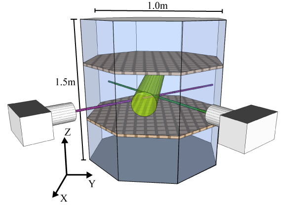
This work is based on optically tracking passive tracer particles seeded in a turbulent flow agitated by two oscillating grids as shown in Fig. 1. For clear measurements of 1-D inhomogeneity a large system is needed to create significant separation for locally homogeneous and inhomogeneous regions, and to create sufficiently high Reynolds numbers. In order to study large scale effects conditional statistics were analyzed, which required large data sets ($>10^{9}$ particle pairs). Storage, speed, and budget concerns led to the development of real time image compression circuits chan:2007 . These devices enabled nearly endless data acquisition for a nominal cost.

II.1 Experimental Apparatus

Turbulence was generated between two identical octagonal grids oscillating in phase in an octagonal Plexiglas tank that is 1m$~{}\times$ 1m$~{}\times$ 1.5m and filled with approximately 1,100 liters (300 gallons) of filtered, degassed water. The grids have 8 cm mesh size, 36% solidity, and were evenly spaced from the top and bottom of the tank with a 56.2 cm spacing between grids and a 1 cm gap between grid and tank walls. The stroke was 12 cm peak to peak, powered by an 11 kW motor. A typical grid frequency was 3 Hz, but was raised to 5 Hz to investigate Reynolds number dependence. Water cooling maintains the temperature at $\pm$ 0.1C during each run. Neutrally buoyant 136 $\mu$m diameter polystyrene tracer particles were added to the flow until approximately 50 were seen by each camera. This particle density was chosen to maximize data per frame while minimizing tracking errors. Particle density could greatly increase with the planned addition of two more cameras ott:1999 ; Dracos:1996:TDV . One difficulty of oscillating grid flows is that vibrations from the oscillatory drive can couple to the camera supports and degrade imaging accuracy. We mounted a custom camera support on an optical table to minimize vibrations. Air bubble suppression was an additional concern. We developed a method to keep all water seals and bearings sufficiently wet to maintain an air tight seal.

Figure 1: Experimental apparatus diagram. Two oscillating grids were held 56.2 cm apart in a 1,100 liter octagonal prism Plexiglas tank. Two high speed cameras are used to stereoscopically image chosen regions of the tank in order to record 3D particle positions. Illumination is provided by a Nd:YAG laser with 50 W average power.

II.2 Detection

These data were acquired using 3D PTV (particle tracking velocimetry) measurements using two Bassler A504K video cameras capable of 1280 $~{}\times$ 1024 pixel resolution at 500 frames per second (a data rate of approximately 625 MB per second per camera). Recording such a high data rate is a significant technological hurdle. A typical system would store data in 4 GB of video RAM, so that one run would last just 7 seconds before waiting approximately 7 minutes for the data to download to hard disk. We use an image compression circuit to threshold images in real-time so that only pixels above a user defined brightness limit are regarded as particle data and retained while the dark background pixels are discarded chan:2007 . This technique produces a dynamic data compression factor of 100-1000, which enables continuous data collection and storage to hard disk.

Our first implementation of the image compression circuits have faced two major challenges. First, the simple thresholding compression reduces particle center accuracy. However, particle finding accuracy is typically degraded by only 0.1 pixel, which is typically less than the uncertainty in particle finding from unthresholded images. Secondly, because frame number information was created and recorded separately on each computer, any operating system delay can lead to frames lost and timing mismatch between the cameras. For the measurements in this paper, frame number errors were corrected in post processing. Updated versions of the image compression circuit have solved this problem by including camera frame number in the data stream the computers record.

Particles are illuminated using a 532 nm pulsed Nd:YAG laser with 50 W average power. The beam was expanded to create an illumination volume approximately 7cm $\times$ 4cm $\times$ 5cm. Images were processed to find the center of each particle as seen by each camera and then stereomatched to find the 3D position in real space. Stereomatching was accurate to approximately 11 $\mu$m (0.08 particle diameters or 0.2 pixels). At this level of accuracy it is essential to have a very good calibration of camera position parameters to use for stereomatching. We start with a traditional calibration to obtain initial 3D stereomatching  Otto:2008 . We then use known stereomatched pairs from the two cameras, and run a non-linear optimization to minimize the stereomatching error and find optimal camera position parameters ott:1999 .

III Results

III.1 Characterizing the Flow

We define a characteristic velocity by $u=(\langle u_{i}u_{i}\rangle/3)^{1/2}$ and a characteristic length scale by $L=u^{3}/\varepsilon$ where $\varepsilon$ is the energy dissipation rate per unit mass defined in section  III.3. For the center region $u=6.0$ cm/s, $L=9.0$ cm, and for the near grid region $u=8.3$ cm/s, $L=4.5$ cm. The Taylor Reynolds number, $R_{\lambda}=(15uL/\nu)^{1/2}$, (where $\nu$ is the kinematic viscosity) ranges from 285 for 3 Hz grid frequency to 380 for 5 Hz grid frequency in the center. Near the grid at 3Hz $R_{\lambda}=230.$ The Kolmogorov length and time scales are $\eta=140\mu$m, $\tau_{\eta}=20$ ms in the center region, and $\eta=94~{}\mu$m, $\tau_{\eta}=8.8$ ms in the near grid region.

Figure 2(a) shows the mean vertical velocity as a function of the vertical position along the central axis of the tank. The top and bottom grids are separated by 56.2 cm, approximately 7 L. In Fig. 2, the dot-dashed line indicates the maximum amplitude of the bottom grid, 22.1 cm below the center of the tank. Data was collected at 5 separate heights in order to measure the complete flow profile from the center of the tank to the bottom grid. Mapping the bottom half of the tank is sufficient because the geometrical symmetry produces a mirror image above the midplane. The two volumes which we will focus on throughout this paper are bounded by the dashed lines, and will be referred to as the center (C), and near grid (NG) observation volumes. At this grid separation distance the mean flow traces four torii, two above and two below the center plane of the tank, as shown in the sketch in figure 3 (drawn to scale). In the large central region, the effect of the mean flow is to pump highly energetic fluid from the region near the grid towards the center of the tank. In figure 2(a), there are two points where the mean vertical velocity reaches zero: one near the center, the other 18 cm from the center just below the near grid observation volume. The existence of this second stagnation point and reverse circulation region depicted in Fig. 3 is a common feature in mean flows generated by oscillations Otto:2008 . In the following measurements, the small mean velocity has been subtracted so that we study the fluctuating velocity field.

Figure 2: Mean and variance of vertical velocity along the central vertical axis of the tank. Grid frequency 3 Hz, grid separation distance 56.2 cm. The dot-dash line represents the grid height at maximum amplitude. The remainder of the paper will focus on measurements in two regions designated by the vertical dashed lines: one at the center of the tank and one near the grid.

Figure 3: Scale diagram of 56cm $\times$ 100cm area between grids showing the mean circulation torii which are nearly rotationally symmetric about the central vertical axis. Center and Near Grid observation volumes are drawn in dashed lines, which shows the relative size and position of the observation volumes in figure 2. Horizontal dot-dashed lines represent range of motion of the top and bottom grids.

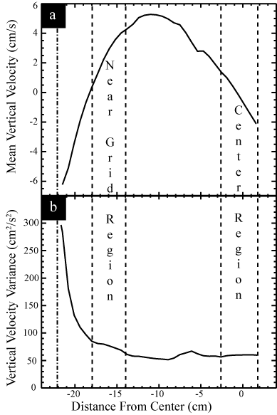
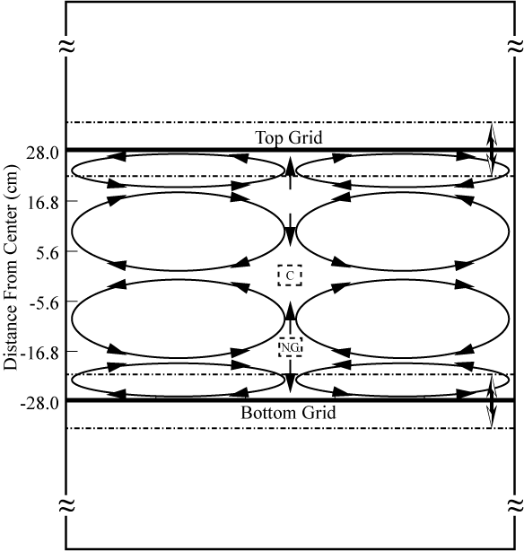
Figure 2(b) shows the vertical velocity variance along the central axis as a function of vertical position. The velocity variance is large near the grid and quickly falls off towards the center where it is nearly homogeneous. The center and near grid observation volumes were chosen to provide a contrast between the large homogeneous region in the center and the much more inhomogeneous region near the grid. In the center, the variance of the velocity is homogeneous for several L in either direction. The velocity variance ranges moderately in the near grid observation volume, and enormously within one L below this region. In Fig. 2, deviations from a smooth curve are not due to statistical uncertainty, but are a result of patching 5 calibrated regions together with the majority of error coming from measuring absolute position in the tank.

It is interesting to note that we made measurements in a flow with a smaller grid separation of 35 cm and found that the Reynolds number in the center was lower. The characteristic velocity in the center did increase due to the closer proximity of the grids, but $L$ was reduced by a larger amount resulting in approximately 8% decrease in $R_{\lambda}$. The reason for the unexpected decrease in Reynolds number is a reversal of the mean velocity compared with larger grid separations. For larger grid separation distances, energetic fluid from near the grids is carried to the center by the mean flow. However, at 35 cm grid separation the mean velocity reverses which results in a lower Reynolds number in the center.

III.2 Structure Functions

Figure 4: Eulerian second order longitudinal velocity structure function shown as a function of pair separation $r$ scaled by the Kolmogorov length $\eta$. The inset shows this data compensated by Eq. 1 for $p$=2.

Figure 5: Eulerian third order longitudinal velocity structure function. The inset shows this data compensated by Eq. 1 for $p$=3.

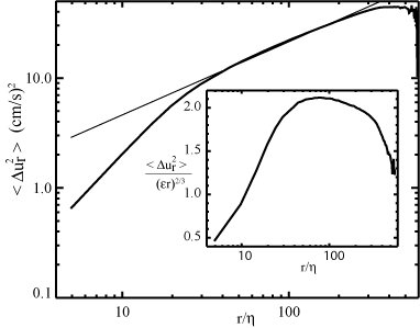
To measure Eulerian structure functions we first find the instantaneous longitudinal velocity difference between two particles a distance $r$ apart $\Delta u_{r}=[\mathbf{u}(\mathbf{x})-\mathbf{u}(\mathbf{x}+\mathbf{r})]_{L}$, where the $L$ subscript denotes the longitudinal component, found by projecting the 3D velocity difference vector onto the vector connecting the two particles. The longitudinal structure functions are defined as $D_{p}=\langle(\Delta u_{r})^{p}\rangle$ where $p$ represents the order of the structure function and the brackets represent the ensemble average. In the inertial range, Kolmogorov (1941) gives

$$\langle\Delta u_{r}^{p}\rangle=C^{(E)}_{p}(\varepsilon r)^{p/3},$$ (1)

where the $C^{(E)}_{p}$ are Eulerian Kolmogorov constants and $\varepsilon$ is the energy dissipation rate.

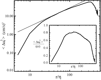
Figures 4 and 5 show the measured second and third order longitudinal velocity structure functions with the straight thin lines representing Kolmogorov’s prediction from Eq. 1. The insets show the structure functions compensated by Eq. 1. At $R_{\lambda}=285$, any scaling range is very limited, but the plateaus can be used to estimate the inertial range.

Lagrangian structure functions were measured from temporal velocity differences along a particle trajectory. The velocity difference now becomes $\Delta u_{\tau}=u(t)-u(t+\tau)$, where $\tau$ is the time interval between measurements. We use the vertical component of the velocity for Lagrangian velocity differences throughout this paper, although results for the other components are similar. For Lagrangian structure functions Kolmogorov (1941) predicts

$$\langle\Delta u_{\tau}^{p}\rangle=C^{(L)}_{p}(\varepsilon\tau)^{p/2}.$$ (2)

III.3 Energy Dissipation Rate Measurement

The energy dissipation rate $\varepsilon$ is an important value throughout this analysis, it is worth a moment to discuss how it is determined. Limitations in particle density preclude direct measurement via the definition

$$\varepsilon=2\nu\langle s_{ij}s_{ij}\rangle$$

with

$$s_{ij}=\frac{1}{2}\left(\frac{\partial u_{i}}{\partial x_{j}}+\frac{\partial u_{j}}{\partial x_{i}}\right).$$

Instead we utilize Kolmogorov’s 4/5 law: Eq. 1 with $p=3$ where the coefficient $C^{(E)}_{3}=-4/5$ can be derived from the Navier-Stokes equations. We identify the inertial range with the plateau in the compensated third order structure function (Fig. 5 inset). The inertial range is chosen to be 25 to 91 $r/\eta$ (.35 to 1.3 cm). If the same inertial range is used in the second order structure function, the energy dissipation rate determined from it (using the empirical coefficient $C^{(E)}_{2}=2.0$) Pope:2000 is within 3% of the value calculated from the third order.

III.4 Phase Dependence

A simple energy cascade has constant energy input at the largest length scales. An obvious departure from constant energy input is the oscillating grid driving mechanism. The sinusoidal motion of the grid directly corresponds to energy input with periodic time dependence. It seems likely that such a strongly periodic energy input would have a signature throughout the whole energy cascade.

The method we employ throughout this work to detect signatures of the large scales is to condition various statistics on some measurement of the state of the large scales. In this case, we condition on the phase of the grid motion, $\phi$. Conditioning instantaneous single particle statistics such as the mean and variance of the velocity shows some sinusoidal dependence on grid phase. For example, in the center the conditional variance, $\langle(u-\langle u\rangle)^{2}|\phi\rangle$, varies by $1\%$ over the cycle of the grid. In the near grid region, the conditional variance varies by $10\%$. The mean vertical velocity in the center, $\langle u|\phi\rangle$, varies by 0.8 cm/s over a cycle of the grid which is 10% of the standard deviation. Near the grid, the conditional mean velocity varies by 2 cm/s, which is 20% of the standard deviation at that location.

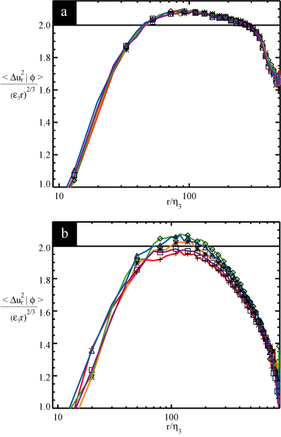
Figure 6 shows the compensated second order longitudinal structure functions conditioned on the phase, $\langle\Delta u_{r}^{2}|\phi\rangle$. In the center of the flow (Fig. 6(a)) the structure functions have essentially no change with phase. Near the grid (Fig. 6(b)) there is a slight dependence on grid phase. To emphasize the differences between structure functions at different phases, we compensated the structure functions by a single energy dissipation rate in each figure, $\varepsilon_{3}=24.6$ cm${}^{2}/$s³ in the center and $\varepsilon_{3}=131$ cm${}^{2}/$s³ near the grid. These values were determined when the grid is in mid amplitude (the third bin). The good collapse of the structure functions at all phases across the entire range of $r$ shows the minimal dependence of the small scales on the large scale periodicity of the flow created by the oscillating grids. One possible source of dependence of small scale statistics on large scales has been shown to be minimal.

Figure 6: (Color Online) Second order compensated velocity structure functions conditioned on grid phase. The collapse shows the very weak phase dependence. a) center of the tank (C). b) near the grid (NG). Zero and 2$\pi$ phase represents grid at lowest possible amplitude. $\phi$: $+$ = 0 - 2$\pi$/5, $\ast$ = 2$\pi$/5 - 4$\pi$/5, $\diamond$ = 4$\pi$/5 - 6$\pi$/5, $\triangle$ = 6$\pi$/5 - 8$\pi$/5 , $\Box$ = 8$\pi$/5 - 2$\pi$.

III.5 Dependence on Large Scale Velocity

III.5.1 Eulerian structure functions conditioned on the large scale velocity: center region

A more revealing dependence on the large scales of the flow is found by conditioning the velocity structure functions directly on the large scale velocity. A convenient measurable quantity that reflects the local instantaneous state of the large scales is the average velocity of the particle pair used for the structure function, defined as $\Sigma u_{z}=(u_{z}(\mathbf{x})+u_{z}(\mathbf{x}+\mathbf{r}))/2.$ Alternatively, conditioning on the average velocity of many particles, not just one pair, was studied and found to have very similar results, but we choose to focus on $\Sigma u_{z}$ because it can be more easily measured and does not depend on the observation volume and seeding density. Additional conditioning quantities will be discussed in section III.7.

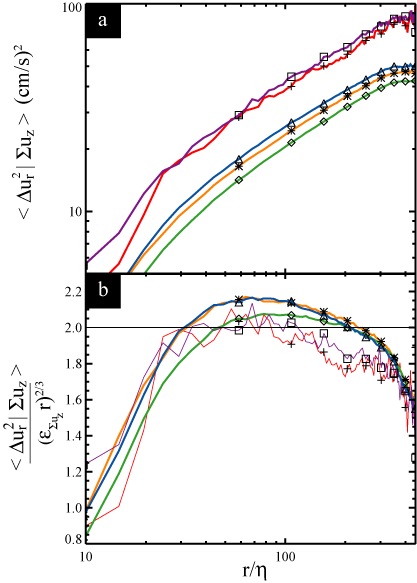
Figure 7(a) shows the second order Eulerian velocity structure function conditioned on $\Sigma u_{z}$. The smallest values of the structure function correspond to pair velocities near zero, represented by $\diamond$, while large $|\Sigma u_{z}|$ results in larger values of the structure functions. For the bins we chose, the structure function conditioned on large values of $\Sigma u_{z}$ is nearly twice the value when conditioned on $\Sigma u_{z}$ near zero.

Figure 7(b) shows the data in Figure 7(a) compensated by Kolmogorov inertial range scaling. The functional forms are quite similar, confirming the impression from Fig. 7(a) that all length scales are affected similarly by the instantaneous state of the large scales. In Fig. 7(b) we used a different energy dissipation rate, $\varepsilon_{u_{z}}$ to compensate each of the 5 individual large scale vertical velocity bins. This insures all conditions plateau at approximately the same value, and allows for direct comparison of the functional forms of the conditional structure functions.

The strong dependence of the conditional structure functions on the large scale velocity at all scales reveals that the small scales are not statistically independent of the large scales in this flow. There is not any detectable trend toward the smaller scales becoming less dependent on the large scale velocity than somewhat larger scales.

Figure 7: (Color online) Second order velocity structure function conditioned on particle pair velocity (vertical component) in the center of the tank. a) Uncompensated structure functions b) Individually compensated by the energy dissipation rate for each conditional data set. Symbols represent the following dimensionless vertical velocities, $\Sigma u_{z}/\sqrt{\langle u_{z}^{2}\rangle}$: $+$ = 4.2 to 2.5, $\ast$ = 2.5 to 0.84, $\diamond$ = 0.84 to -0.84, $\triangle$ = -0.84 to -2.5, $\Box$ = -2.5 to -4.2.

Figure 8: (Color online) Second order Lagrangian velocity structure function conditioned on instantaneous velocity (vertical component) in the center of the tank. a) Uncompensated structure functions. b) Individually compensated to have the peak values match. Symbols represent the following dimensionless vertical velocities, $\Sigma u_{z}/\sqrt{\langle u_{z}^{2}\rangle}$: $+$ = 3.1 to 1.9, $\ast$ = 1.9 to 0.62, $\diamond$ = 0.62 to -0.62, $\triangle$ = -0.62 to -1.9 , $\Box$ = -1.9 to -3.1.

III.5.2 Lagrangian structure functions conditioned on the large scale velocity: center region

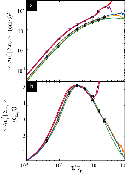
In much the same way we can evaluate the conditional Lagrangian structure functions. Figure 8(a) shows the second order Lagrangian structure function conditioned on the vertical component of the large scale velocity, $\Sigma u_{z}$. Here we find $\Sigma u_{z}$ by averaging the velocity of the particle at the two times used to determine $\Delta u_{\tau}$. The conditional structure functions for different large scale velocity are different by a factor of about 2.5, and they remain nearly parallel throughout the entire time range.

Figure 8(b) shows the second order conditional Lagrangian structure function compensated by Eq. 2 where $\varepsilon$ is individually chosen so the maxima of all of the conditioned structure functions coincide. This aids comparison of the functional forms of the conditioned structure functions. Again, the functional form is nearly identical for different large scale velocities, indicating that the large scales affect all time scales in the same way. There may be a small trend towards larger values of the compensated Lagrangian structure functions at small times when the magnitude of the large scale velocity is large.

It should be noted that there is a bias present in Lagrangian measurements that is not present in Eulerian measurements. A sample of measured Lagrangian trajectories is biased towards low velocity particles since the high velocity particles are more likely to have left the measurement volume. This bias becomes larger for larger $\tau$. Berg et al.. Berg:2009 have studied this bias and find that it can be quite large for typical experimental conditions. We quantified this bias in our data by measuring the Lagrangian structure functions using trajectories that remained inside artificially restricted measurement volumes. From a simple extrapolation of the dependence on the size of the artificial detection volume, we estimate that our experimental Lagrangian structure functions underestimate the true value by 17% for $\tau=8\tau_{\eta}$. This is roughly consistent with the size of the error we expect based on the critical time lag defined in Ref. Berg:2009 . Note that we have not performed the compensation they recommend and we are roughly translating their uncompensated results. Because of this bias, we will focus attention on $\tau<10\tau_{\eta}$. As we’ll discuss in section III.6.3, the dependence of the conditioned Lagrangian structure functions on the large scale velocity does not seem to be significantly influenced by this bias.

III.5.3 Eulerian structure functions conditioned on the large scale velocity: near grid region

By comparing separate regions of the tank we are able to explore the effects of inhomogeneity on this conditional dependence. Figure 9 shows the Eulerian structure functions, similar to Fig. 7, but with data collected in the inhomogeneous region near the bottom grid (NG). The separation between Eulerian structure function conditions has doubled to approximately a factor of four. Note the different ordering of the structure functions. The up-down symmetry is now broken. Fluid traveling upwards ($*$ symbols) has a large structure function while fluid traveling downward with the same magnitude of vertical velocity ($\triangle$ symbols) has the lowest value of the structure function. We interpret this as highly energetic fluid originating near the bottom grid and being turbulently advected into the observation volume. Similarly, fluid carried down from the more quiescent region above the detection volume has low energy and a smaller structure function.

Figure 9: (Color online) Second order velocity structure function conditioned on particle pair vertical velocity (Z direction) in the region near the bottom grid. The condition with the largest downward velocity has been eliminated due to lack of statistical convergence. Symbols represent the following particle pair vertical velocities $\Sigma u_{z}/\sqrt{\langle u_{z}^{2}\rangle}$: $+$ = 3.8 to 2.3, $\ast$ = 2.3 to 0.75, $\diamond$ = 0.75 to -0.75, $\triangle$ = -0.75 to -2.3, a) Uncompensated structure functions b) Individually compensated by the energy dissipation rate for each conditional data set.

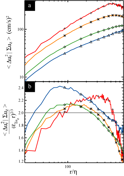
Figure 9(b) shows the compensated Eulerian structure functions, similar to figure 7(b), but reveals a novel insight. Stepping through the vertical velocity bins is equivalent to stepping through the energy cascade. Fluid coming directly upward from the bottom grid (symbol $+$) carries energy that was recently injected into the large scales. As a result, the compensated structure function for upward moving fluid is biased towards the large scales. Fluid that has downward vertical velocity (symbol $\triangle$) comes from the center region far away from the grid. It has had more time to mature, and in this process the energy is transported to smaller length scales. Conditional structure functions appear to be an effective tool to evaluate whether or not a turbulent flow is fully developed and has established a stable cascade.

Figure 10: (Color online) Third order velocity structure function plots conditioned on particle pair vertical velocity and individually compensated for each conditional data set. Data is taken in the center region of the tank, and the extreme vertical velocity plots have been eliminated due to lack of statistical convergence. Symbols represent the following vertical velocities $\Sigma u_{z}/\sqrt{\langle u_{z}^{2}\rangle}$: $\ast$ = 2.5 to 0.84, $\diamond$ = 0.84 to to -0.84, $\triangle$ = -0.84 to -2.5.

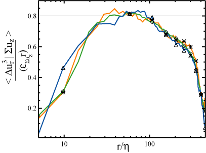
III.5.4 Third order Eulerian structure functions conditioned on the large scale velocity: center region

Figure 10 shows the third order structure function individually compensated and conditioned on $\Sigma u_{z}$ in the center of the tank. Convergence of third order statistics was more difficult, so elimination of the two extreme conditions was required. The third order structure function proves to be similar to the second order in separation, symmetry, and collapse to a single functional form. The energy dissipation rates found for the three conditions are: $\varepsilon_{\ast}=25.2$cm${}^{2}/$s³, $\varepsilon_{\diamond}=21.7$cm${}^{2}/$s³,$\varepsilon_{\triangle}=28.7$cm${}^{2}/$s³.

III.6 A Powerful Method for Plotting Conditional Structure Functions

III.6.1 Eulerian structure functions conditioned on the large scale velocity: center region

An alternative, and in many ways a more powerful, method of visualizing the same data is presented in Fig. 11. Here we show the second order Eulerian structure function conditioned on the vertical component of the large scale velocity (the same data as Fig. 7). However, the scaled vertical pair velocity is plotted on the horizontal axis with conditioned structure functions on the vertical axis. When the structure functions are scaled by their value at $\Sigma u_{z}=0$, we find very good collapse of the data. The fact that these curves for different $r/\eta$ collapse so well is a striking demonstration that the large scales affect all length scales in the same way. The fact that the conditional structure functions vary by a factor of 2.5 demonstrates the strong dependence on the large scales. Note that for Gaussian random fields, the plot in Fig. 11 would be flat, and a nearly flat result is observed in DNS and grid turbulence sreenivasan:1998 .

Figure 11: (Color Online) Eulerian second order conditional structure function versus large scale velocity. Data taken in the center region. Each curve represent the following separation distances $r/\eta$: $+$ = 0 to 40, $\ast$ = 40 to 70, $\diamond$ = 70 to 110, $\triangle$ = 110 to 140, $\Box$ = 300 to 370, $\times$ = 370 to 440.

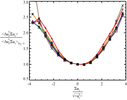
In Fig. 11, it may be expected that the structure function at the largest length scales ($\times$) are a function of the large scale velocity. We see here that the dependence is a steep parabola. What is now more clear with this plotting method is the extent to which all the smaller scales are also affected by the large scale velocity; in fact, all length scales collapse nearly perfectly onto one parabola. The large scale velocity affects all length scales in nearly the exact same way, all the way down to the dissipative range.

Figure 12: (Color Online) Eulerian second order conditional structure function versus large scale velocity. Data taken in the center region at higher grid frequency, 5Hz, resulting in higher Taylor Reynolds number  380. Symbols represent the following separation distances $r/\eta$: $+$ = 0 to 50, $\ast$ = 50 to 100, $\diamond$ = 100 to 150, $\triangle$ = 150 to 200, $\Box$ = 310 to 420, $\times$ = 420 to 520.

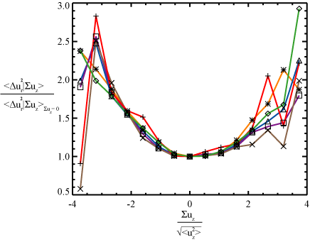
III.6.2 Eulerian structure functions conditioned on the large scale velocity: higher Reynolds number

Figure 12 shows the effect of increasing the Reynolds number. This data is at the center of the tank with the grids oscillating at 5 Hz which increases $R_{\lambda}$ to 380. The collapse of the structure function remains. The curvature in this figure is not significantly different from the lower Reynolds number data in Fig. 11 indicating that if there is a Reynolds number dependence it is weak.

Figure 13: (Color Online) Eulerian second order conditional structure function versus large scale velocity. The thin plots are from atmospheric boundary layer data  sreenivasan:1998 $r/\eta$: $\ast$ $\thicksim$ 100, $\triangle$ $\thicksim$ 400, $\Box$ $\thicksim$ 1000, $\times$ $\thicksim$ 1250. The thick line is from fig. 11, which has been overlaid for comparison, $r/\eta$: $\diamond$ = 70 to 110.

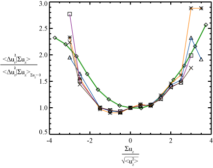
Figure 13 shows a comparison of our data with data taken in the atmospheric boundary layer sreenivasan:1998 with $R_{\lambda}>10^{4}$. Atmospheric boundary layer turbulence shows a similar collapse of conditional structure functions at all length scales. The curvature is also similar in both data sets, indicating that the dependence on the large scales is similar even at these very large Reynolds numbers.

Figure 14: (Color Online) Lagrangian second order conditional structure function versus large scale vertical velocity. Data taken in the center region. Symbols represent the following $\tau/\tau_{\eta}$: $+$ = 0.42 , $\ast$ = 1.3, $\diamond$ = 3.5, $\triangle$ = 10.

III.6.3 Lagrangian structure functions conditioned on the large scale velocity: center region

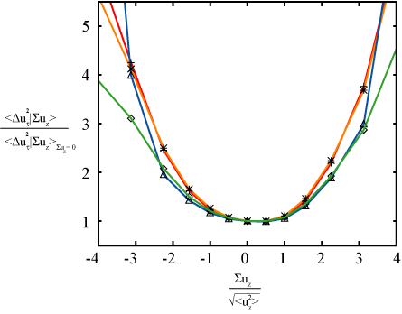
Figure 14 shows the Lagrangian structure functions plotted versus the large scale velocity, comparable to the Eulerian data shown in Fig. 11. The parabolic shape remains, but the curvature is greater for all Lagrangian time scales than it is in the Eulerian data. All time scales are affected by the large scale velocity. To determine the effect of measurement volume bias, we have done this analysis for artificially restricted measurement volumes. By decreasing the volume by a factor of 2, we observe the large $\tau$ curves to shift by approximately the deviations between the curves. We conclude that the bias does not have a significant effect on the conditional dependence shown in Fig. 14 for the time differences presented ($\tau\leq 10\tau_{\eta}$).

Figure 15: (Color Online) Eulerian second order conditional structure function versus large scale velocity. Data taken in the near grid region of the tank. The structure function is heavily influenced by the bottom grid which has skewed the symmetry of the plot minima in the negative direction. Symbols represent the following non-dimensional separation distances $r/\eta$: $+$ = 0 to 50, $\ast$ = 50 to 110, $\diamond$ = 110 to 160, $\triangle$ = 270 to 320, $\Box$ = 330 to 450, $\times$ = 450 to 560.

III.6.4 Eulerian structure functions conditioned on the large scale velocity: near grid region

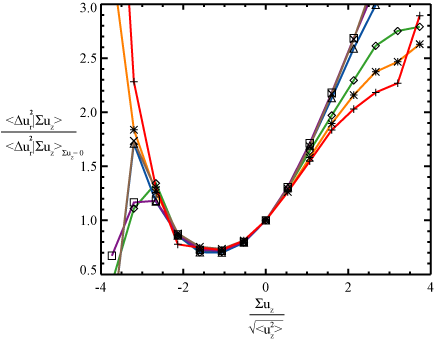
Figure 15 shows conditioned Eulerian structure function similar to figure 11, but measured in the inhomogeneous region near the grid (NG). The structure functions here are strikingly different than in the center. The minimum is shifted by more than one standard deviation to the left. The inhomogeneity breaks the up-down symmetry so that fluid coming directly up from the bottom grid is markedly different then fluid coming down from the more quiescent region above (analogous to the $*$ and $\triangle$ separation in Fig. 9). It follows that fluid with an upward velocity has higher energy than fluid with the same velocity magnitude in the downward direction. The atmospheric boundary layer data in Fig. 13 also shows this effect with a minimum at $\Sigma u_{z}/\sqrt{\langle u_{z}^{2}\rangle}=-0.5$, presumably as a result of weaker inhomogeneity. Also notable is that the collapse of plots for various $r$ values is not as complete as in the central region. This is consistent with Fig. 9(b) which shows that the conditional structure functions have somewhat different $r$ dependence.

Figure 16: (Color Online) Lagrangian second order conditional structure function versus large scale vertical velocity. Data taken in the near grid region of the tank. Symbols represent the following $\tau/\tau_{\eta}$: $+$ = 0.94, $\ast$ = 2.8, $\diamond$ = 8.0.

III.6.5 Lagrangian structure functions conditioned on the large scale velocity: near grid region

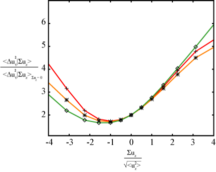
Figure 16 shows a Lagrangian structure function taken in the near grid region, similar to the Eulerian data in Fig. 15. The minimum is shifted to the left here also as a result of the inhomogeneity in this region of the flow. The conditional dependence on the large scale velocity is again somewhat larger than in the Eulerian case, and the collapse at different time scales is not as complete.

Figure 17: (Color Online) Eulerian third order conditional structure function versus large scale vertical velocity in the center region. Symbols represent the following non-dimensional separation distances $r/\eta$: $+$ = 0 to 40, $\ast$ = 40 to 70, $\diamond$ = 70 to 110, $\triangle$ = 110 to 140, $\Box$ = 220 to 300, $\times$ = 300 to 370.

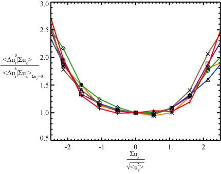
III.6.6 Third order Eulerian structure functions conditioned on the large scale velocity: center region

The third order Eulerian velocity structure function plotted versus the large scale vertical velocity is shown in Fig. 17 using data from the center of the tank. Statistical convergence is weaker than the second order which limits the large scale velocity range available for analysis. The collapse seems similar to the second order case shown in Fig. 11, although the measurement uncertainties are larger here. The curvature seems to be slightly larger for the third order than for the second order case.

Figure 18: (Color Online) Eulerian second order conditional structure function versus magnitude of the velocity pair in the center region. Symbols represent the following non-dimensional separation distances $r/\eta$: $+$ = 0 to 40, $\ast$ = 40 to 70, $\diamond$ = 70 to 110, $\triangle$ = 110 to 140, $\Box$ = 300 to 370, $\times$ = 370 to 440.

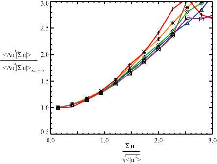
III.6.7 Second order Eulerian structure functions conditioned on the velocity magnitude: center region

The second order Eulerian structure function plotted versus the magnitude of the pair velocity is shown in Fig. 18 using data from the center observation volume. The magnitude of the pair velocity is also a useful indicator of large scale activity. It has no preferred direction, and it is a more direct indicator of the instantaneous local energy. A similar dependence remains as in Fig. 11, the collapse seems similar, and the curvature is significantly larger.

III.7 Discussion

We have provided a comprehensive set of measurements that shows signatures of the current state of the large scales on the inertial range and small scales in turbulence. Here we wish to discuss factors that might be responsible for the dependence of structure functions on the instantaneous large scale velocity. First we will address a possible concern that the conditional dependence may be a kinematic correlation. Then we will discuss possible properties of the large scales that could be important including Reynolds number, anisotropy, mean shear, inhomogeneity, and large scale intermittency. We do not claim that this list is exhaustive, but it seems that identifying the major contributors will be valuable.

A reasonable suspicion might be that the observed dependence is a kinematic correlation, meaning that particle pairs with large velocity may also have a large velocity difference simply because the same measurements are used in both cases. Hosokawa Hosokawa:2007 identified that Kolmogorov’s 4/5ths law requires that velocity sums and differences be correlated so that

$$\langle u_{+}^{2}\Delta u_{-}\rangle=\frac{\epsilon r}{30}$$ (3)

where $u_{-}$ is half the longitudinal velocity difference and $u_{+}$ is half the sum. (For comparison, we have used $\Delta u_{r}=2u_{-}$ and below $\Sigma u_{\parallel}=u_{+}.$) Khomyansky Tsinober:2008 et al provide an experimental confirmation of this and in a more recent paper Tsinober:preprint present a list of kinematic relations. However, several lines of evidence indicate that kinematic correlation does not account for the majority of the dependence we observe.

First, note that two independent random samples with identical Gaussian distributions have a difference that is uncorrelated with the sum, so that the conditional dependence seen in Fig 11 would be flat. This remains true for velocity differences and sums from Gaussian random fields. Both of these results can be obtained by considering the joint pdf of the two samples, and then rotating 45 degrees to the coordinate system of sums and differences. Because the samples are interchangeable, the sum and difference axes have to be principle axes of the joint gaussian pdf, and the conditional variance of the difference is independent of the sum.

Of course, turbulent velocities are not joint Gaussian. However, from the kinematic relations in the literature we have not been able to derive predictions for the conditional structure functions that we consider or for the correlation $\langle(\Sigma u)^{2}(\Delta u)^{2}\rangle$ that would capture the main conditional dependence we see.

To make an experimental estimate of the effect of kinematic correlations, we conditioned the velocity differences on several other quantities. For each particle pair, we calculated the longitudinal and transverse components of the average velocity of the particles, denoted $\Sigma u_{\parallel}$ and $\Sigma u_{\perp}$ respectively. We then conditioned the longitudinal structure functions on the longitudinal and transverse pair velocities instead of conditioning on the pair vertical velocity. The idea here is that while conditioning the longitudinal structure functions on the longitudinal component ($\Sigma u_{\parallel}$) could have a kinematic correlation, conditioning on the transverse component ($\Sigma u_{\perp}$) should have no kinematic correlation. We found that conditioning on ($\Sigma u_{\parallel}$) had a roughly 30% larger effect on the structure functions than conditioning on ($\Sigma u_{\perp}$). Conditioning on $\Sigma u_{z}$ should have less kinematic correlation than conditioning on $\Sigma u_{\parallel}$. So more than 70% of the effect remains unexplained by kinematic correlation. We conclude that while kinematic correlation may possibly make a significant contribution to the conditional dependence, the majority of the effect comes from the large scales.

An immediate concern when discussing large scale effects is if the oscillating grid flow has a Reynolds number insufficient for adequate scale separation, and it is this which leads to contamination of the small scale statics by the large scales. Evidence points to large scale dependence not being caused by limited Reynolds number. The comparison in Fig. 13 shows that atmospheric boundary layer data sreenivasan:1998 with very large Reynolds number ($R_{\lambda}>10^{4}$) has nearly the same dependence on the large scales as our flow. Increasing the Reynolds number in our flow makes very little difference. Additionally, all length scales collapse to nearly the same functional form indicating that limited separation of scales is not the primary factor. Taken together, these lead us to the conclusion that merely high Reynolds number alone is not enough to create small scales that are statistically independent of the large scales.

Our flow is somewhat anisotropic. The ratio of vertical to horizontal velocity standard deviations is 1.5:1 in the center. The effects of large scale anisotropy on the small scales has been studied extensively biferale:1999 , but it is not a major factor in conditional dependence studied here. We have analyzed our data by averaging over particle pairs with all orientations, so when the structure functions are conditioned on a quantity with no preferred direction like the velocity magnitude (Figure  18) there should be very little contribution from anisotropy. In fact, we find that the conditional dependence on velocity magnitude is even stronger than the dependence on the vertical velocity component. We also observe the conditional dependence remains when conditioned on other quantities without preferred directions like $\Sigma u_{\parallel}$, and $\Sigma u_{\perp}$. We conclude that anisotropy of the large scales is not a significant cause of the conditional dependence we observe.

Sreenivasan and Dhruva sreenivasan:1998 attribute the strong conditional dependence of the Eulerian structure functions on the large scale velocity to shear in the atmospheric boundary layer. In making this argument, they show an important piece of information in their figure 6 which shows conditioned structure functions in homogeneous turbulence from both DNS and wind tunnel grid turbulence. The conditional statistics in these homogeneous and isotropic flows show no apparent dependence on the large scale velocity. However, we conclude that shear is not the fundamental property responsible in our flow since the oscillating grid flow has a much lower shear but produces much the same dependence on the large scale velocity. The mean velocity gradient normalized with the eddy turnover time is 1.2 in the center of our flow and we estimate it is in the range of 5 or greater for their atmospheric boundary layer data. There must be some other properties that exist in the shear flow, but also are important in our flow with small shear.

Our data clearly shows the role that inhomogeneity plays in the observed large scale dependence. Our Eulerian and Lagrangian data near the grid in Figs. 15 and 16 show that the structure functions depend greatly on the origin of the fluid being swept into the observation volume. Fluid coming from energetic regions of the tank have larger structure functions than fluid coming from more quiescent regions. Inhomogeneity is directly responsible for the shift of the minimum in Fig. 15 away from zero vertical velocity. In the center of the tank (Fig. 11), the inhomogeneity is much smaller, but it could be responsible for part of the curvature since both fluid coming downward and fluid coming upward would be coming from more energetic regions symmetrically.

However, inhomogeneity alone does not account for all of the large scale dependence observed. There is also a significant contribution from large scale intermittency, and it is possible that this is the dominant contribution in the center of the tank. Large scale intermittency has been difficult to quantify. It can be defined as any temporal fluctuations in the large scales that occur on timescales longer than the eddy turnover time, $L/u$.

Fernando and DeSilva Fernando:1993 show large scale intermittency can exist in an oscillating grid flow depending on boundary conditions. We have observed clear signatures of large scale intermittency in our flow. Although we use their recommended boundary conditions, the velocity distribution in the center of the flow is slightly bimodal indicative of switching between two flow states. This effect is more prominent in preliminary data we took for grid spacings of 66 cm and 100 cm than it is in the data for 56.2cm presented in this paper.

Our measurements show a dependence of the conditional structure functions on the large scale velocity that can not be fully attributed to inhomogeneity, and large scale intermittency appears to be the most likely cause. The clearest evidence for this comes from conditioning the structure functions on the horizontal components of the large scale velocity, $\Sigma u_{x}$ and $\Sigma u_{y}$ instead of on the vertical component, $\Sigma u_{z}$. The horizontal midplane ($x$ and $y$ directions) is much more homogeneous than the vertical axis (z direction). Yet, the structure functions conditioned on $\Sigma u_{y}$ or $\Sigma u_{x}$ show a large scale dependence that is only moderately smaller than for the $\Sigma u_{z}$ condition (85% and 72% of the dependence seen in $\Sigma u_{z}$). If the inhomogeneous direction shows similar conditional dependence on the large scales as the homogeneous directions show, then it seems that a large part of the conditional dependence must come from fluctuations in the large scales, and not directly from inhomogeneity. Praskovsky et al. Praskovsky:1993 attribute large scale intermittency as a crucial component of the large scale dependence they observe. More work is needed to isolate the effects of large scale intermittency on small scale statistics in turbulence.

We have largely ignored considerations of power law scaling which has been a focus of much of the previous work on this subject. Because of the relatively low Reynolds number of our experiment, we can not make sensitive tests of scaling. However, our data provides a plausible picture about how the large scales should affect power law scaling. If the data in Fig. 11 collapses to a single curve, then the dependence of the conditional structure functions on $r$ and $u_{z}$ are separable and the large scale dependence will have no effect on the scaling exponents of unconditional structure functions. When this type of plot does not collapse as in Figs. 15 and  16, then the power law scaling will be affected by the large scales.

IV Conclusions

We study a flow between oscillating grids with 3D particle tracking and a novel real-time image compression system in order to quantify the effects of various properties of the non-universal large scales on the inertial range and small scales.

We measured the mean and variance of the velocity as a function of distance from the grids. The oscillating grid motion has produced a weak mean flow as well as a region near the grid with high velocity variance that falls off quickly to a very homogeneous, lower velocity variance, region in the center. This profile has been key in the determination of the role of inhomogeneity.

Conditional statistics were employed in order to measure the large scale effects. Second order Eulerian velocity structure functions were conditioned on the phase of the grid, an obvious source for periodic large scale energy input. Results show little dependence of the structure functions in the center region and surprisingly little even near the grid.

Eulerian and Lagrangian structure functions were also conditioned on the instantaneous large scale velocity. A large dependence was found in the center, with the Eulerian structure function increasing by a factor of 2 or more when the large scale velocity is large. The dependence of the Lagrangian structure functions is somewhat larger. Conditioned structure functions show that in the center of the tank, all length scales are affected in approximately the same way. The region near the grid was also analyzed and compared with the region in the center. Near the grid, we found a much stronger dependence on the instantaneous large scale velocity for both the Eulerian and Lagrangian structure functions than we found in the center. Near the grid, there are clear signatures of the effects of large scale inhomogeneity on the small scales. Fluid coming up from the energetic region nearer the grid has large structure functions, while fluid coming down from the quiescent region in the center has much smaller structure functions. The functional form of the conditional structure functions are also different indicating the different histories of the different fluid. These measurements provide a clear picture of the way inhomogeneity affects the small scales of turbulence.

Plotting the conditional structure functions versus the large scale velocity provides a powerful method for visualizing the effects of the large scales on all length scales in turbulent flows. We recommend these plots as an effective way to compare the effects of the large scales in different experiments. This has been done for grid turbulence and homogeneous, isotropic DNS sreenivasan:1998 which show almost no dependence of the structure functions on large scale velocity. Our oscillating grid flow and high Reynolds number atmospheric boundary layer turbulence sreenivasan:1998 show very similar dependence. Comparison of conditional structure functions in other flows has the potential to clarify the effects of the large scales on small scale turbulence and to guide the search for universal properties of turbulent flows.

V Acknowledgements

This work was supported by Wesleyan University, the Alfred P. Sloan foundation, and NSF grant DMR-0547712. We thank Rachel Brown, Emmalee Riegler and Tom Glomann for assistance with the experiment. We benefitted from discussions with Nick Ouellette, Haitao Xu, Eberhard Bodenschatz, Zellman Warhaft, Laurent Mydlarski, and Mark Nelkin.

References

- (1) K. R. Sreenivasan and R. A. Antonia. The phenomenology of small-scale turbulence. Annu. Rev. Fluid Mech., 29:435, 1997.
- (2) A Arneodo, C Baudet, F Belin, R Benzi, B Castaing, B Chabaud, R Chavarria, S Ciliberto, R Camussi, F Chilla, B Dubrulle, Y Gagne, B Hebral, J Herweijer, M Marchand, J Maurer, JF Muzy, A Naert, A Noullez, J Peinke, F Roux, P Tabeling, W vandeWater, and H Willaime. Structure functions in turbulence, in various flow configurations, at reynolds number between 30 and 5000, using extended self-similarity. Europhys. Lett., 34:411, 1996.
- (3) L. Biferale, E. Bodenschatz, M. Cencini, A.S. Lanotte, N.T. Ouellette, F. Toschi, and H. Xu. Lagrangian structure functions in turbulence: A quantitative comparison between experiment and direct numerical simulation. Physics of Fluids, 20:065103, 2008.
- (4) NT Ouellette, HT Xu, M Bourgoin, and E Bodenschatz. Small-scale anisotropy in Lagrangian turbulence. New J Physics, 8:102, 2006.
- (5) Luca Biferale and Frederico Toschi. Anisotropic homogeneous turbulence: Hierarchy and intermittency of scaling exponents in the anisotropic sectors. Physical Review Letters, 86:4831, 2001.
- (6) X Shen and Z Warhaft. The anisotropy of the small scale structure in high reynolds number turbulent shear flow. Phys. of Fluids, 12:2976, 2000.
- (7) Federico Toschi and Eberhard Bodenschatz. Lagrangian properties of particles in turbulence. Annu. Rev. Fluid Mech., 41:375, 2009.
- (8) S Douady, Y Couder, and ME Brachet. Direct observation of the intermittency of intense vorticity filaments in turbulence. Physical Review Letters, 67:983, 1991.
- (9) Greg A. Voth, A. La Porta, Alice M. Crawford, Jim Alexander, and Eberhard Bodenschatz. Measurement of particle accelerations in fully developed turbulence. Journal of Fluid Mechanics, 469:121, 2002.
- (10) N. Mordant, P. Metz, O. Michel, and J Pinton. Measurement of lagrangian velocity in fully developed turbulence. Physical Review Letters, 87:214501, 2001.
- (11) H.J.S. Fernando and I.P. DeSilva. Note on secondary flows in oscillating-grid, mixing-box, experiments. Physics of Fluids, A5:1849, 1993.
- (12) I.P. DeSilva and H.J.S. Fernando. Oscillating grids as a source of nearly isotropic turbulence. Physics of Fluids, 6:2455, 1994.
- (13) Soren Ott and Jakob Mann. An experimental investigation of the relative diffusion of particle pairs in three-dimensional turbulent flow. Journal of Fluid Mechanics, 422:207, 2000.
- (14) E.A. Variano and E.A. Cowen. A random jet stirred turbulence tank. Journal of Fluid Mechanics, 64:1, 2008.
- (15) Beat Luethi, Soren Ott, Jacob Berg, and Jakob Mann. Lagrangian multi-particle statistics. Journal of Turbulence, 8:1, 2007.
- (16) Vedula Prakash and P.K Yeung. Similarity scaling of acceleration and pressure statistics in numerical simulations of isotropic turbulence. Physics of Fluids, 11(5), 1999.
- (17) N. Mordant, A.M. Crawford, and E. Bodenschatz. Experimentally lagrangian acceleration probability density function measurement. Physica D, 193:245, 2004.
- (18) Alexander A. Praskovsky, Evgeny B. Gledzer, Mikail Yu Karyakin, and Ye Zhou. The sweeping decorrelation hypothesis and energy-inertial scale interaction in high reynolds number flows. Journal of Fluid Mechanics, 248:493, 1993.
- (19) Katepalli R. Sreenivasan and Brindesh Dhruva. Is there scaling in high-reynolds-number turbulence? Progress of Theoretical Physics, 130:103, 1998.
- (20) Greg Voth. Lagrangian acceleration measurements in turbulence at large Reynolds numbers. Ph.D. Thesis, Cornell University, 2000.
- (21) B.L. Sawford, P.K. Yeung, M.S. Borgas, P. Vedula, A. La Porta, A.M. Crawford, and E. Bodenschatz. Measurement of particle accelerations in fully developed turbulence. Physics of Fluids, 15(11), 2003.
- (22) K. R. Sreenivasan. On local isotropy of passive scalars in turbulent shear flows. Proc. Royal Soc. London, 434:165, July 1991.
- (23) Itai Arad, Victor S. L’vov, and Itamar Procaccia. Correlation functions in isotropic and anisotropic turbulence: The role of the symmetry group. Phys. Rev. E, 59:6753, 1999.
- (24) Itai Arad, Luca Biferale, Irene Mazzitelli, and Itamar Procaccia. Disentangling scaling properties in anisotropic and inhomogeneous turbulence. Physical Review Letters, 82:5040, 1999.
- (25) Dennis Chan, Dominik Stich, and Greg A. Voth. Real time image compression for high-speed particle tracking. Review of Scientific Instruments, 78:023704, 2007.
- (26) Jakob Mann, Soren Ott, and Jacob Sparre Andersen. Experimental study of relative, turbulent diffusion. RISO internal report, Roskilde Denmark, R-1036, 1999.
- (27) T. Dracos. Three-Dimensional Velocity and Vorticity Measuring and Image Analysis Techniques. Kluwer, Dordrecht, Netherlands, 1996.
- (28) Florian Otto, Emmalee K. Riegler, and Greg A. Voth. Measurements of the steady streaming flow around oscillating spheres using three dimensional particle tracking velocimetry. Physics of Fluids, 20:093304, 2008.
- (29) Stephen B. Pope. Turbulent Flows. Cambridge University Press, 2000.
- (30) Jacob Berg, Søren Ott, Jakob Mann, and Beat Lüthi. Experimental investigation of lagrangian structure functions in turbulence. Phys. Rev. E, 80:026316, 2009.
- (31) Iwao Hosokawa. A paradox concerning the refined similarity hypothesis of kolmogorov for isotropic turbulence. Prog. Theor. Phys. Letters, 118:169, 2007.
- (32) Michael Kholmyansky and A Tsinober. Kolmogorov 4/5 law, nonlocality, and sweeping decorrelation hypothesis. Phys. of Fluids, 20:041704, 2008.
- (33) Michael Kholmyansky, V. Sabelnikov, and A Tsinober. New developments in field experiments in ASL: Kolmogorov 4/5 law and non-locality. 18th Symposium on Boundary Layers and Turbulence, http://ams.confex.com/ams/18BLT/techprogram/paper_139408.htm, 2008.