Effect of CO desorption and coadsorption with O on the phase diagram of a Ziff-Gulari-Barshad model for the catalytic oxidation of CO
Abstract
We study the effect of coadsorption of CO and O on a Ziff-Gulari-Barshad (ZGB) model with CO desorption (ZGB-d) for the reaction CO + O CO2 on a catalytic surface. Coadsorption of CO at a surface site already occupied by an O is introduced by an Eley-Rideal-type mechanism that occurs with probability , . We find that, besides the well-known effect of eliminating the second-order phase transition between the reactive state and an O-poisoned state, the coadsorption step has a profound effect on the transition between the reactive state and the CO-poisoned state. The coexistence curve between these two states terminates at a critical value of the desorption rate which now depends on . Our Monte Carlo simulations and finite-size scaling analysis indicate that decreases with increasing values of . For , there appears to be a sharp phase transition between the two states only for at (or near) zero.
pacs:
82.65.+r, 68.43.De, 05.50.+q, 05.10.LnI Introduction
Catalytic reactions on surfaces are very complex, and their comprehensive understanding is vital, both for its intrinsic scientific interest and for its immense technological applications. bond87 ; chri94 The scientific interest is due to the emergence of a rich and complex variety of phenomena, including chaotic behavior, bistability, critical phenomena, out-of-equilibrium phase transitions, etc. bond87 ; marro99 Due to its crucial role in industrial applications, the oxidation of CO on a transition-metal catalyst is one of the most studied reactions. In a pioneering work, Ziff, Gulari and Barshad (ZGB) ziff86 proposed a deceptively simple model to describe some kinetic aspects of the reaction CO + O CO2 on a catalytic surface in terms of a single parameter , which represents the probability that the next molecule arriving at the surface is a CO, i.e.,., it is proportional to the partial pressure of CO. The model exhibits two kinetic phase transitions, one continuous, at , between an oxygen-poisoned phase and a reactive one, and a discontinuous one, at , between a reactive phase and a CO poisoned one. Unfortunately, there are important aspects of this catalytic reaction that are not reproduced by this simple model. Transitions between states of low and high CO coverage, (the fraction of surface sites occupied by CO), have been observed experimentally. ehsa89 At low temperatures, as increases, there is a discontinuous drop in the CO2 production rate; while above a certain critical temperature the discontinuity disappears, and the CO2 production decreases continuously. This type of behavior can be reproduced by including a CO desorption rate, , the so-called ZGB-d model.kauk89 ; alba92 ; bros92 Another feature that is erroneously predicted by the original ZGB model is the continuous phase transition at , since experiments show that the reaction rate increases as soon as the CO concentration departs from zero. ehsa89 The real system does not present an oxygen-poisoned state because oxygen does not impede the adsorption of CO. ertl90 ; kris92 Several authors have shown that this transition can be eliminated by adding to the Langmuir-Hinshelwood (LH) mechanism that defines the original ZGB model an Eley-Rideal (ER) step that allows a reaction between CO molecules in the gas phase and adsorbed O atoms on the surface. meak90 ; tamb94 However, there are no experimental data indicating that such a reaction between free CO and adsorbed oxygen occurs, but there is experimental evidence that suggests that under certain conditions, it is possible that a CO molecule can be weakly adsorbed at a site already occupied by an oxygen atom. camp80 Experiments based on photoemission electron microscopy have shown that CO can be adsorbed on a saturated O surface. huan02 This coadsorption is a prerequisite for the reaction to happen, and it can be simulated by an ER-type mechanism that occurs with a certain probability. Some previous work on the ZGB model with coadsorption indicates that the production rate of CO2 increases linearly with (in the region of low ), and that the continuous phase transition from the reactive state to the O poisoned state disappears. meak90 ; huad02 ; qais04 ; mukh09 In these works it was assumed that the addition of the ER-type step does not alter the nature of the transition at , but simply shifts it to a lower value of .
We believe that the effect of the ER-type step on the ZGB-model deserves a more detailed analysis. In this work we therefore explore what happens when a coadsorption mechanism is added to the ZGB model with CO desorption. For the ZGB-d model, there is a distinction between the high and low CO-coverage phases only for desorption rates below some critical value , while above the CO coverage varies smoothly with . Thus, the transition value becomes a function of , corresponding to a coexistence curve that terminates at the critical point . tome93 ; ziff92 ; mach05 The value of has been estimated by several authors. An earlier work based on fractal scaling of the interface between phases indicates that the first-order phase transition disappears for .bros92 More recent estimates based on the probability distribution for the CO coverage (histograms), the fourth-order cumulant, and finite-size scaling theory give the values ,tome93 and ,mach05 respectively. In this work we are particularly interested in studying how the nature of the transition at changes when the ER-type mechanism is added with probability to the ZGB-d model. To the best of our knowledge, such an analysis has not been performed previously. Our study is based on kinetic Monte Carlo simulations and finite-size scaling analysis of the data.
The rest of this paper is organized as follows. In Sec. II, we define the model and describe the Monte Carlo simulation techniques used. In Sec. III A, we present and discuss the numerical results obtained for the case of . In Sec. III B, we perform a finite-size scaling analysis for the particular case of the standard ZGB model with an Eley-Rideal step (). Our conclusions are summarized in Sec. IV.
II Model and Simulation
The ZGB model with desorption and coadsorption is simulated on a square lattice of linear size that represents the catalytic surface. A Monte Carlo simulation generates a sequence of trials: CO or O2 adsorption with probability and CO desorption with probability . For the adsorption a CO or O2 molecule is selected with probability and respectively. ziff86 ; tome93 These probabilities are the relative impingement rates of both molecules and are proportional to their partial pressures. The algorithm works in the following way. A site is selected at random. For desorption, if is occupied by CO the site is vacated; if not, the trial ends. For adsorption, if a CO molecule is selected it can be adsorbed at an empty site if none of its nearest neighbors are occupied by an O atom. Otherwise, one of the neighbors occupied by O is selected at random and removed from the surface, leaving and the selected neighbor vacant. This move simulates the CO + O CO2 surface reaction following the adsorption of CO. If the selected site is occupied by an O atom the CO is coadsorbed with probability , and a CO2 molecule is liberated leaving behind an empty site on the surface. This represents the ER reaction. O2 molecules can be adsorbed only if a pair of nearest-neighbor sites are vacant. If the adsorbed molecule is selected to be O2, a nearest neighbor of , , is selected at random, and if it is occupied the trial ends. If both and are empty, the trial proceeds, and the O2 molecule is adsorbed and dissociates into two adsorbed O atoms. If none of the remaining neighbors of is occupied by a CO molecule, the one O atom is located at , and if none of the neighbors of is occupied by a CO molecule, then the other O is located at . If any neighbors of are occupied by a CO, then one is selected at random to react with the O at such that both sites are vacated. The same reaction happens at site if any of its neighbors are filled with a CO molecule. This process mimics the CO + O CO2 surface reaction following O2 adsorption. A schematic representation of this algorithm is given by
| CO(a) | ||||
| CO(a) | ||||
Here represents an empty site on the surface, means gas phase, means adsorbed, and means coadsorbed. The first three steps correspond to the LH mechanism, the fourth step to the CO desorption, and the last two steps to the ER-type mechanism, which occurs with probability . If , we recover the ZGB-d model, if , we have the ZGB-d model with an ER step. It is important to realize that the ER reactions are essentially instantaneous, so that the CO cannot remain coadsorbed without reacting.
For our simulations we assume periodic boundary conditions. The time unit is one Monte Carlo Step per Site, MCSS, in which each site is visited once, on average. Averages are taken over independent simulation runs for each set of parameters.
III Results
Starting from an empty lattice, we wait until the system reaches a steady state at constant partial pressure . We calculate the fraction of sites occupied by CO molecules: the CO coverage, ; the O coverage, , and the fraction of empty sites, . is the rate of production of CO2.
III.1 Results for
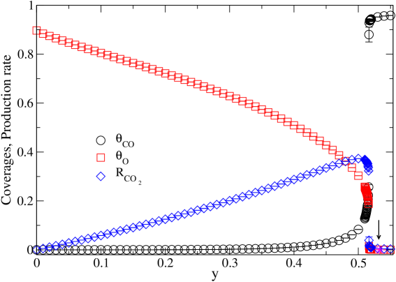
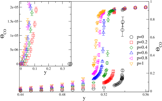
In Fig. 1, we show the dependence of the coverages and the CO2 production rate on the CO pressure, , for the particular case of and . It is immediately seen that the inclusion of the ER-type step () has a dual effect: one is to eliminate the oxygen-saturated phase and therefore the continuous transition at in the ZGB model, and the other is that the transition to a CO-saturated surface occurs at a lower value of the CO pressure than for . These two effects can be seen in more detail in Fig. 2, where we plot the CO coverage vs for a fixed value of and different values of . As increases, the second transition is shifted toward lower values of , and the CO coverage starts to increase as soon as , except for the case (the ZGB-d model), in which it starts at . A closer scrutiny of Fig. 2 also reveals that the discontinuity in at appears to become smaller as increases, giving way to a continuous change for below approximately .
Previous studies show that when CO desorption () is added to the original ZGB model, the ZGB-d model, the discontinuous transition ends at a critical value , such that in this case . tome93 ; ziff92 ; mach05 . To the best of our knowledge, there have been no studies of how the nature of the transition changes when an ER-type step is added to the ZGB-d model, and this is the main topic we explore in this paper.
An efficient way to locate and classify phase transitions is to look at the fourth-order reduced cumulant of the order parameter. For it takes the form, mach05 ; land00 ; bind84 ; challa86
| (1) |
where
| (2) |
is the th central moment of the CO coverage, and is the probability distribution for . This probability distribution is obtained by counting the number of times, , that the coverage falls in the intervals (), such that is the total number of MCSS. Then, the probability, , that has a value in the interval is
| (3) |
such that
| (4) |
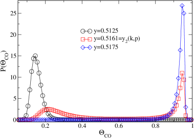
In Fig. 3 we show for fixed values of and , and values of in different regions: below and above , where the histograms are unimodal, indicating that the system consists of one single phase, and at where the histograms are bimodal, signaling the existence of two distinct phases. At the coexistence point , the areas under both peaks are equal. borg90 ; land00 A finite-size scaling analysis would have to be performed to ascertain if the transition is continuous or discontinuous for any particular values of and . Such a study is planned for future work.
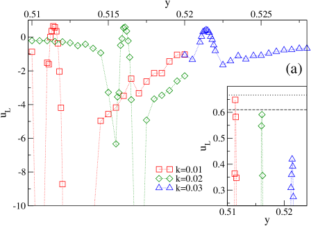
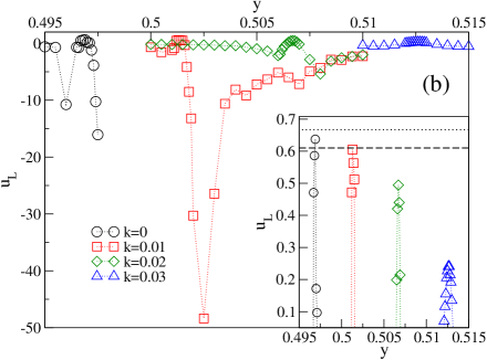
The equal-area bimodal distribution corresponding to coexistence yields a positive maximum for the cumulant vs , flanked on either side by negative minima and approaching zero far away from the transition. The maxima of define the -dependent coexistence line, . In Fig. 4 we show the dependence of on for several values of of and (Fig. 4(a)), and (Fig. 4(b)). In the proximity of a first-order phase transition, the maximum value of the fourth-order cumulant (when ) takes the value of ,bind81 while for a continuous transition the maximum takes a lower value. For the Ising universality class, the maximum value of at the critical point is approximately 0.61. kami93 Our results strongly suggest that when the ER-type step is added () the coexistence curve ends at some value of that decreases when increases, i.e., now . Figure 4(a) indicates that when , the first-order phase transition seems to terminate at some value of below 0.02, i.e., , while Fig. 4(b) indicates that even for the well-known ZGB model (, no desorption) with , meak90 it is not clear that the transition remains first-order. In the following we analyze this particular case in further detail.
III.2 Results for
The standard ZGB model with the addition of an ER step has been analyzed by several authors, meak90 ; tamb94 ; huad02 ; qais04 ; mukh09 but as far as we know the nature of the transition at has not been studied in detail, and it has been assumed that, besides destroying the continuous transition at , the effect of the extra step is simply to shift the first-order transition to a lower value of . Our analysis of the fourth-order cumulant suggests that is depressed by increasing , and in this section we perform finite-size scaling analysis to further investigate this point.
The fluctuations of can be calculated in the standard way as
| (5) |
where
| (6) |
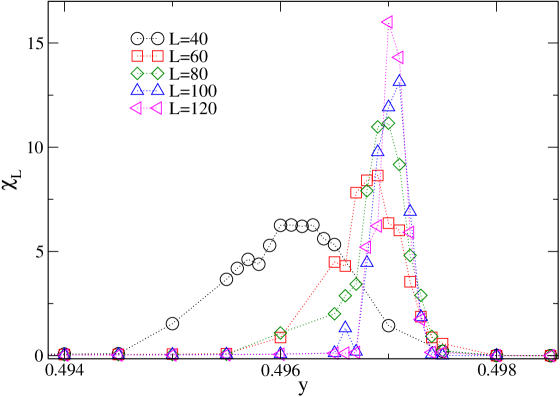
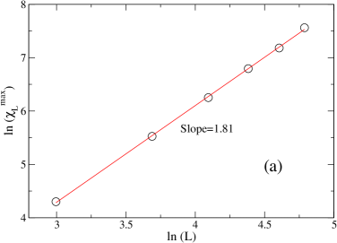
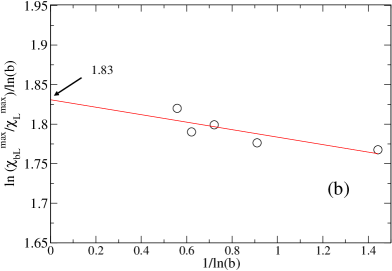
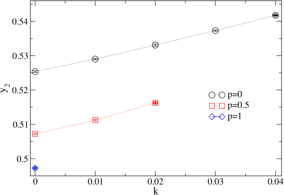
The peak positions of approach the infinite-system transition point with increasing . In Fig. 5 we show as a function of for and for several values of . As expected, the peaks of the curves shift and increase in height with increasing . It is well known that at a first-order equilibrium phase transition the order parameter fluctuations scale as , where is the spatial dimension of the system (here ). nien75 ; fish82 ; land00 Previously we have successfully used the same scaling relation to identify the nonequilibrium first-order transition in the ZGB-d model.mach05 In Fig. 6(a) we plot ln() vs ln(). The linear fit indicates a power-law scaling, such that , where . We also measure the power-law exponent by a different method, which has some advantage in eliminating the effects of a nonsingular background term (as in with and constants). We write
| (7) |
with fixed at a relatively small value (here, ), and . For large and , the correction term is proportional to , so that the exponent can be estimated by plotting the left-hand-side of Eq. (7) vs and extrapolating to , as in Fig. 6(b). The resulting estimate is . These results are relatively far from the expected value for a first-order phase transition, in clear contrast with the exponent calculated by the same techniques for , in which case we found that for the transition at . mach05 This analysis provides further support to our previous suggestion, based on the fourth-order cumulant, that the ZGB model with an ER step () does not have a phase transition but only a smooth crossover for any non-zero value of .
IV Conclusions
In this paper we have presented a study of the ZGB-d model in which an ER-type step is added (). The extra step can be thought of as a way to include a surface interaction between CO and O coadsorbed at the same site. We found that, besides eliminating the unphysical oxygen-poisoned state and therefore the second-order transition of the original ZGB model, the inclusion of the ER-type step has a more profound effect than the mere shifting of the first-order transition at toward lower values, which was previously reported in the literature. meak90 ; tamb94 ; huad02 The addition of the ER-type step changes the nature of the transition between the CO2 producing phase and the non-productive CO-poisoned phase, in such a way that now the coexistence curves terminate at a value of that decreases with . Even for the well-studied case of the ZGB with an ER mechanism (), our results indicate that it is not legitimate to speak of a phase transition at for any non-zero . These results are summarized in Fig. 7, where we show a rough estimate of the coexistence curves indicating for some values of the upper value of for which there could still exist a first-order phase transition. We hope our results will be of use for the analysis of experiments on heterogeneous CO oxidation.
Acknowledgments
G.M.B is grateful for the hospitality of the Physics Department and the Center for Materials Research and Technology at Florida State University. P.A.R acknowledges support by U.S. National Science Foundation Grant No. DMR-0802288.
References
- (1) G. C. Bond, Catalysis: Principles and Applications (Clarendon, Oxford, 1987).
- (2) K. Christmann, Introduction to Surface Physical Chemistry (Steinkopff Verlag, Darmstadt, 1991); V. P. Z. Zhdanov and B. Kazemo, Surf. Sci. Rep. 20, 111 (1994).
- (3) J. Marro and R. Dickman, Nonequilibrium Phase Transitions in Lattice Models (Cambridge University Press, Cambridge, 1999).
- (4) R. M. Ziff, E. Gulari, and Y. Barshad, Phys. Rev. Lett. 56, 2553 (1986).
- (5) M. Ehsasi, M. Matloch, O. Frank, J. H. Block, K. Christmann, F. S. Rys, and W. Hirschwald, J. Chem. Phys. 91, 4949 (1989).
- (6) H. P. Kaukonen and R. M. Nieminen, J. Chem. Phys. 91, 4380 (1989).
- (7) E. V. Albano, Appl. Phys. A: Solids Surf. 54, 2149 (1992).
- (8) B. J. Brosilow and R. M. Ziff, Phys. Rev. A 46, 4534 (1992).
- (9) G. Ertl, Adv. Catal. 37 213 (1990).
- (10) K. Kischer, M. Eiswirth, and G. Ertl, J. Chem. Phys. 96, 9161 (1992).
- (11) P. Meakin, J. Chem. Phys. 93, 2903 (1990).
- (12) S. S. Tambe, V. K. Yayaraman, and B. D. Kulkarni, Chem. Phys. Lett. 225, 303 (1994).
- (13) C. T. Campbell, G. Ertl, H. Kuipers, and G. Segner, J. Chem. Phys. 73, 5862 (1980).
- (14) X. X. Huang, X. H. Bao, H. H. Rotermund, and G. Ertl, J. Phys. Chem. B 106, 5645 (2002).
- (15) D. Y. Hua and Y. Q. Ma, Chin. Phys. Lett. 19, 534 (2002).
- (16) A. U. Qaisrani, M. Khalid and M. Kaleen Baloch, Chin. Phys. Lett. 21, 1838 (2004).
- (17) A. K. Mukherjee and I. Sinha Appl. Surf. Sci. 255, 6168 (2009).
- (18) T. Tomé and R. Dickman, Phys. Rev. E 47, 948 (1993).
- (19) R. M. Ziff and B. J. Brosilow, Phys. Rev. A 46, 4630 (1992).
- (20) E. Machado, G. M. Buendía and P. A. Rikvold, Phys. Rev. E 71, 031603 (2005).
- (21) D. P. Landau and K. Binder, A Guide to Monte Carlo Simulations in Statistical Physics (Cambridge University Press, Cambridge, 2000).
- (22) K. Binder and D. P. Landau, Phys. Rev. B 30, 1477 (1984).
- (23) M. S. Challa, D. P. Landau, and K. Binder, Phys. Rev. B 34, 1841 (1986).
- (24) C. Borgs and R. Kotecký, J Stat. Phys. 61, 79 (1990).
- (25) K. Binder, Phys. Rev. Lett. 47, 693 (1981); Z. Phys. B 43, 119 (1981).
- (26) B. Nienhuis and M. Nauenberg, Phys. Rev. Lett. 35, 477 (1975).
- (27) M. E. Fisher and A. N. Berker, Phys. Rev. B 26, 2507 (1982).
- (28) G. Kamieniarz and H. W. J. Blöte, J. Phys. A 26, 201 (1993).