Nonlinear non-extensive approach for identification of structured information

Abstract

The problem of separating structured information representing phenomena of differing natures is considered. A structure is assumed to be independent of the others if can be represented in a complementary subspace. When the concomitant subspaces are well separated the problem is readily solvable by a linear technique. Otherwise, the linear approach fails to correctly discriminate the required information. Hence, a non extensive approach is proposed. The resulting nonlinear technique is shown to be suitable for dealing with cases that cannot be tackled by the linear one.

1 Introduction

We consider the problem of discriminating information produced by phenomena of differing natures, via inverse methods. This involves the study of the physical state of a system by analyzing its response to some external interaction. We refer to the interactive carrier as input signal and to the system’s reaction as signal response. Unfortunately, a particular response is not always directly available, as one may receive it ‘disguised’ by the interference with another independent phenomenon not being the focus of specific interest. In this paper we restrict our consideration to responses evoked by statistical systems. By this we understand systems which are fully characterized by of a probability distribution indicating either the population of subsystems compressing the whole system, or the degree of uncertainty about the system being in one of its possible states. We regard both situations to be identical in the description and refer to subsystems as system’s states.

In order to formulate the problem let us use the label ‘$i$’, ranging from 1 to $M$, to denote the $i$-th state of a system which is characterized by a probability $p_{i}$. Adopting Dirac’s notation we indicate by a ket $|f_{\cal{V}}\rangle$ the system’s response to some input signal and by $|v_{i}\rangle$ the corresponding response of the $i$-th state. Consequently, the system’s signal response satisfies

$$|f_{\cal{V}}\rangle\propto\sum_{i=1}^{M}p_{i}|v_{i}\rangle.$$

This equation is transformed into an equality by simply relaxing the condition $\sum_{i=1}^{M}p_{i}=1$, so that

$$|f_{{\cal{V}}}\rangle=\sum_{i=1}^{M}c_{i}|v_{i}\rangle,$$

where the coefficients in the superposition are not necessarily normalized to unity. As already stated, we are interested in the problem of discriminating $|f_{\cal{V}}\rangle$ from a given signal $|f\rangle$ of which $|f_{\cal{V}}\rangle$ is a component. Out of the many situations involving this problem it immediately comes to our mind the intensity of X-rays produced simultaneously by dispersion and diffraction or an infrared emission spectrum superimposed to blackbody radiation. In order to model all relevant cases we assume that, rather than $|f_{{\cal{V}}}\rangle$, the available signal is $|f\rangle=|f_{{\cal{V}}}\rangle+|f_{{\cal{W}^{\bot}}}\rangle$, where $|f_{{\cal{W}^{\bot}}}\rangle$ is produced by an independent phenomenon. We focus on those cases ensuring a unique decomposition, i.e., we further assume that the subspaces hosting the components $|f_{{\cal{V}}}\rangle$ and $|f_{{\cal{W}^{\bot}}}\rangle$ are complementary. However, the focus of our interest refers to complementary subspaces being close enough together to move the problem of separating the components far away from the trivial one. Certainly, if the subspaces hosting the signal components are well separated, the problem is readily solvable by means of an oblique projection onto one of the subspaces and along the other [1, 2]. Contrarily, if the subspaces are not well separated the construction of the necessary projector becomes ill posed and the problem needs to be tackled in an alternative way. In this Communication we address the matter by including a hypothesis upon the system producing the signal response. We assume that the population of states is $K$-sparse in the sense that, out of the $M$ possible states of the system, only $K<M$ of them are characterized by a significant probability. Nevertheless, the hypothesis generates, in general, an intractable problem, because of course the populated states are unknown and the number of possibilities of populating $K$ states out of $M$ is a combinatorial number $\tbinom{M}{K}$. This makes the exhaustive search for the unknown states an impossible task for most values of $M$ and $K$. In recent publications [3, 4] a greedy strategy for making the search tractable has been proposed. In the present context, the proposal of that publications implies to assume a priori that no state is populated and looks for the populated ones in a stepwise manner. Here we investigate the possibility of addressing the problem from the opposite view point. Assuming a priori that all the states are equally populated, we will determine the actual population of each state via the minimization of the $q-$norm like quantity $\sum_{i=1}^{M}|c_{i}|^{q},\quad 0<q\leq 1.$ The minimization of this quantity as an appropriate criterion for determining a sparse solution to an under-determined linear system is discussed in [5, 6]. For nonnegative and normalized to unity coefficients $c_{i},i=1,\ldots,M$, this quantity is closely related to the non-extensive entropic measure broadly applied in physics [7, 8, 9, 10, 11, 12] since Tsallis introduced it as the essential ingredient of his thermodynamic analysis framework [7]. In the present context the value of $q$ plays a particular role. By choosing $0<q\leq 1$ we introduce an assumption on the sought distribution. We assume that not all the possible states in a system’s model are significantly populated. This assumption is meant to compensate for the actual overestimation of possibilities one usually makes when a system’s signal response is modelled mathematically.

The paper is organized as follows: Section 2 introduces the mathematical setting of the problem and discusses the construction of oblique projectors. Section 3 remarks the need for nonlinear approaches to separate signal components living in subspaces which are ‘theoretically’ complementary, but close enough to prevent the components discrimination being realized by a linear operation. The proposed strategy, based on the minimization of the $q$-norm^q $\sum_{i=1}^{M}|c_{i}|^{q}$, subject to recursively selected constraints, is discussed in Section 4 and illustrated in the same section by a numerical simulation. The numerical experiment is especially designed to highlight the robustness of the proposed approach against significant error in the data. The conclusions are presented in Section 5.

2 Mathematical setting of the problem

As already mentioned, adopting Dirac’s notation we represent the response of a statistical system to some external interaction as $|f_{\cal{V}}\rangle$, which is expressible in the form

$$|f_{{\cal{V}}}\rangle=\sum_{i=1}^{M}c_{i}|v_{i}\rangle.$$ (1)

Since the kets are elements of an inner product space, their square norm is induced by the inner product, i.e., $\||f_{{\cal{V}}}\rangle\|^{2}=\langle f_{{\cal{V}}}|f_{{\cal{V}}}\rangle$.

The problem we are concerned with entails to ‘rescue’ a ket response $|f_{{\cal{V}}}\rangle$ from an available mixture $|f\rangle=|f_{{\cal{V}}}\rangle+|f_{{\cal{W}^{\bot}}}\rangle$, where $|f_{{\cal{W}^{\bot}}}\rangle$ is produced by an independent phenomenon (e.g. a structured interference that one would call background referring to a persistent effect out of the focus of the main interest).

Denoting ${\cal{V}}=\text{span}\{|v_{i}\rangle\}_{i=1}^{M}$ and assuming that the subspace ${\cal{W}^{\bot}}$ such that $|f_{{\cal{W}^{\bot}}}\rangle\in{\cal{W}^{\bot}}$ is known, we restrict considerations to the case ${\cal{V}}\cap{\cal{W}^{\bot}}=\{0\}$ so as to ensure the uniqueness of the decomposition $|f\rangle=|f_{{\cal{V}}}\rangle+|f_{{\cal{W}^{\bot}}}\rangle$. Such a problem has a straightforward ‘theoretical’ solution. Certainly, from $\hat{E}_{{\cal{V}}{\cal{W}^{\bot}}}$, the oblique projector onto ${\cal{V}}$ along ${\cal{W}^{\bot}}$, one immediately has

$$\hat{E}_{{\cal{V}}{\cal{W}^{\bot}}}|f\rangle=\hat{E}_{{\cal{V}}{\cal{W}^{\bot}}}(|f_{{\cal{V}}}\rangle+|f_{{\cal{W}^{\bot}}}\rangle)=|f_{{\cal{V}}}\rangle.$$

However, as will be discussed in the next section, when the subspaces ${\cal{V}}$ and ${\cal{W}^{\bot}}$ are not well separated the numerical construction of $\hat{E}_{{\cal{V}}{\cal{W}^{\bot}}}$ becomes ill posed, thus preventing the signal separation to be correctly realized.

2.1 Construction of Oblique Projections

Let us recall that every idempotent operator is a projector. Hence, an operator $\hat{E}$ is a projector if $\hat{E}^{2}=\hat{E}$. The projection is along its null space and onto its range. When these subspaces are orthogonal $\hat{E}$ is called an orthogonal projector, and it is the case if and only if $\hat{E}$ is self-adjoint. Otherwise it is called an oblique projector. For a good and amusing introduction to oblique projectors in the context of signal processing we refer to [13] and for advanced theoretical study of oblique projector operators in infinite dimensional spaces to [14, 15]. Here we will restrict ourselves to issues related to numerical constructions.

Assuming that ${\cal{V}}\cap{\cal{W}^{\bot}}=\{0\}$ the oblique projector operator onto ${\cal{V}}$ along ${\cal{W}^{\bot}}$ will be represented as above. Then $\hat{E}_{{\cal{V}}{\cal{W}^{\bot}}}$ satisfies $\hat{E}_{{\cal{V}}{\cal{W}^{\bot}}}^{2}=\hat{E}_{{\cal{V}}{\cal{W}^{\bot}}}$ and, consequently,

$$\hat{E}_{{\cal{V}}{\cal{W}^{\bot}}}|g\rangle = |g\rangle,\quad\text{if}\quad|g\rangle\in{\cal{V}}$$

$$\hat{E}_{{\cal{V}}{\cal{W}^{\bot}}}|g\rangle = 0,\quad\text{if}\quad|g\rangle\in{\cal{W}^{\bot}}.$$

In the particular case for which ${\cal{W}^{\bot}}={\cal{V}}^{\bot}$ the operator $\hat{E}_{{\cal{V}}{\cal{V}^{\bot}}}$ is an orthogonal projection onto ${\cal{V}}$. For indicating an orthogonal projector onto a subspace, ${\cal{X}}$ say, we use the particular notation $\hat{P}_{\cal{X}}.$

Given ${\cal{V}}$ and ${\cal{W}^{\bot}}$, in oder to construct $\hat{E}_{{\cal{V}}{\cal{W}^{\bot}}}$ we define $\SS$ as the direct sum of ${\cal{V}}$ and ${\cal{W}^{\bot}}$, which we express as

$$\SS={\cal{V}}\oplus{\cal{W}^{\bot}}.$$

Let ${\cal{W}}=({\cal{W}^{\bot}})^{\bot}$ be the orthogonal complement of ${\cal{W}^{\bot}}$ in $\SS$. Thus we have $\SS={\cal{V}}\oplus{\cal{W}^{\bot}}={\cal{W}}\oplus^{\bot}{\cal{W}^{\bot}},$ where the operation $\oplus^{\bot}$ indicates the orthogonal sum referring to the direct sum of orthogonal subspaces. Assuming that a set $\{y_{j}\}_{j=1}^{J}$ spanning ${\cal{W}^{\bot}}$ is known, we can always construct the orthogonal projector $\hat{P}_{{\cal{W}^{\bot}}}$ to be expressed in the form

$$\hat{P}_{{\cal{W}^{\bot}}}=\sum_{j=1}^{J^{\prime}}|o_{j}\rangle\langle o_{j}|,\,J^{\prime}\leq J,$$

where vectors $\{|o_{j}\rangle\}_{j=1}^{J^{\prime}}$ span ${\cal{W}^{\bot}}$ and are orthonormal, while the given set $\{|y_{i}\rangle\}_{j=1}^{J}$ is not necessarily orthogonal, nor even linearly independent.

From the set $\{|v_{i}\rangle\}_{i=1}^{M}$, spanning ${\cal{V}}$, a spanning set for ${\cal{W}}$ is readily obtained as

$$|u_{i}\rangle=|v_{i}\rangle-\hat{P}_{{\cal{W}^{\bot}}}|v_{i}\rangle=\hat{P}_{{\cal{W}}}|v_{i}\rangle,\,i=1,\ldots,M.$$ (2)

Denoting by $\{|i\rangle\}_{i=1}^{M}$ the standard orthonormal basis for $\mathbb{C}^{M}$, operators $\hat{V}:\mathbb{C}^{M}\to{\cal{V}}$ and $\hat{U}:\mathbb{C}^{M}\to{\cal{W}}$ are defined as

$$\hat{V}=\sum_{i=1}^{M}|v_{i}\rangle\langle i|,\;\;\;\;\;\;\;\;\;\;\;\;\;\;\hat{U}=\sum_{i=1}^{M}|u_{i}\rangle\langle i|.$$

Consequently, the adjoint operators $\hat{U}^{\ast}$ and $\hat{V}^{\ast}$ are

$$\hat{V}^{\ast}=\sum_{i=1}^{M}|i\rangle\langle v_{i}|,\;\;\;\;\;\;\;\;\;\;\;\;\;\ \hat{U}^{\ast}=\sum_{i=1}^{M}|i\rangle\langle u_{i}|.$$

Since $\hat{P}_{{\cal{W}}}\hat{V}=\hat{U}$ and $\hat{U}^{\ast}\hat{P}_{{\cal{W}}}=\hat{U}^{\ast}$, the operator $\hat{G}:\mathbb{C}^{M}\to\mathbb{C}^{M}$ given below

$$\hat{G}=\hat{U}^{\ast}\hat{V}=\hat{U}^{\ast}\hat{U}$$

is a self-adjoint operator. The elements of its matrix representation are

$$\langle i|\hat{G}|j\rangle=\langle u_{i}|v_{j}\rangle=\langle u_{i}|u_{j}\rangle,\,i,j=1,\dots,M.$$

In terms of the above defined operators the oblique projector $\hat{E}_{{\cal{V}}{\cal{W}^{\bot}}}$ is expressed as

$$\hat{E}_{{\cal{V}}{\cal{W}^{\bot}}}=\hat{V}\hat{G}^{\dagger}\hat{U}^{\ast}$$ (3)

or, equivalently,

$$\hat{E}_{{\cal{V}}{\cal{W}^{\bot}}}=\sum_{i=1}^{M}|v_{i}\rangle\langle w_{i}|,$$ (4)

where

$$\langle w_{i}|=\langle i|\hat{G}^{\dagger}\hat{U}^{\ast}=\sum_{j=1}^{M}\langle i|\hat{G}^{\dagger}|j\rangle\langle u_{j}|=\sum_{j=1}^{M}{g}^{\dagger}_{i,j}\langle u_{j}|.$$ (5)

with ${g}^{\dagger}_{i,j}=\langle i|\hat{G}^{\dagger}|j\rangle$ the element $(i,j)$ of a matrix $G^{\dagger}$ indicating the pseudo inverse of $\hat{G}$. It is actually straightforward to verify that $\hat{E}_{{\cal{V}}{\cal{W}^{\bot}}}$ given in (4) satisfies the required properties. Namely, i)$\hat{E}_{{\cal{V}}{\cal{W}^{\bot}}}^{2}=\hat{E}_{{\cal{V}}{\cal{W}^{\bot}}}$, ii) $\hat{E}_{{\cal{V}}{\cal{W}^{\bot}}}|f_{{\cal{V}}}\rangle=|f_{{\cal{V}}}\rangle$, for all $|f_{{\cal{V}}}\rangle\in{\cal{V}}$, and iii)$\hat{E}_{{\cal{V}}{\cal{W}^{\bot}}}|g\rangle=0$ or all $|g\rangle\in{\cal{W}^{\bot}}.$

Note: The condition ${\cal{V}}\cap{\cal{W}^{\bot}}=\{0\}$ implies that the dimension of ${\cal{V}}$ is equal to the dimension of ${\cal{W}}$. Accordingly, if the spanning set $\{|v_{i}\rangle\}_{i=1}^{M}$ is linearly independent, operator $\hat{G}$ has an inverse. Nevertheless, the independence of $\{|v_{i}\rangle\}_{i=1}^{M}$ is not required, so that an inverse for $\hat{G}$ need not exist. For the sake of generality we use $\hat{G}^{\dagger}$, which it is equal to $\hat{G}^{-1}$ when such an inverse does exist.

Let us stress that, since operators $\hat{V}$ and $\hat{U}$ are given in terms of spanning sets for the spaces ${\cal{V}}$ and ${\cal{W}}$, respectively, any such spanning sets can be used. This possibility yields a number of different ways of computing $\hat{E}_{{\cal{V}}{\cal{W}^{\bot}}}$, all of them, of course, theoretically equivalent but not necessarily numerically equivalent when the problem is ill posed.

Considering that $|\psi_{n}\rangle\in\mathbb{C}^{M},\,n=1,\ldots,M$, are the eigenvectors of $\hat{G}$ and assuming that there exist $N$ nonzero eigenvalues $\lambda_{n},\,n=1,\ldots,N$, on taking these eigenvalues in descending order we can express the matrix elements of the Moore-Penrose pseudo inverse of $\hat{G}$ as:

$$\hat{G}^{\dagger}=\sum_{n=1}^{N}|\psi_{n}\rangle\frac{1}{\lambda_{n}}\langle\psi_{n}|.$$ (6)

Moreover, the orthonormal vectors

$$|\xi_{n}\rangle=\frac{\hat{U}|\psi_{n}\rangle}{\sigma_{n}},\quad\sigma_{n}=\sqrt{\lambda_{n}},\quad n=1,\ldots,N$$ (7)

are singular vectors of $\hat{U^{\ast}}$, which satisfy $\hat{U}^{\ast}|\xi_{n}\rangle=\sigma_{n}|\psi_{n}\rangle$, as it is immediate to verify. By defining now the vectors $|\eta_{n}\rangle,\,n=1,\ldots,N$ as

$$|\eta_{n}\rangle=\frac{\hat{V}{|\psi_{n}\rangle}}{\sigma_{n}},\quad\,n=1,\ldots,N,$$ (8)

the projector $\hat{E}_{{\cal{V}}{\cal{W}^{\bot}}}$ in (4) is recast as

$$\hat{E}_{{\cal{V}}{\cal{W}^{\bot}}}=\sum_{n=1}^{N}|\eta_{n}\rangle\langle\xi_{n}|.$$ (9)

Proposition 1.

The vectors $|\xi_{n}\rangle\in{\cal{W}},\,n=1,\ldots,N$ and $|\eta_{n}\rangle\in{\cal{V}},\,n=1,\ldots,N$ given in (7) and (8) are biorthogonal to each other and span ${\cal{W}}$ and ${\cal{V}}$, respectively.

The proof of the above proposition is given in Appendix A.

It is immediate to verify that the representation (4) of $\hat{E}_{{\cal{V}}{\cal{W}^{\bot}}}$ also arises from (9), since

$$|w_{i}\rangle=\sum_{n=1}^{N}|\xi_{n}\rangle\frac{1}{\sigma_{n}}\langle\psi_{n}|i\rangle,\quad i=1,\ldots,M.$$ (10)

Moreover, the representation (4) can be numerically realized in different ways by using different spanning sets to compute the operator $\hat{G}$. Indeed, by orthogonalizing $\{|u_{i}\rangle\}_{i=1}^{M}$ to obtain the orthogonal set $\{|q_{i}\rangle\}_{i=1}^{M^{\prime}},\,M^{\prime}\leq M$ also spanning ${\cal{W}}$, the matrix elements of operator $\hat{G}_{q}$ (replacing $\hat{G}$) are given as $\langle q_{i}|v_{j}\rangle$ (or equivalently as $\langle q_{i}|u_{j}\rangle)\,i,j=1,\ldots,M$. Thus, vectors $\langle w_{i}|$ in (4) are calculated as $\langle w_{i}|=\sum_{j=1}^{M^{\prime}}\langle i|\hat{G_{q}}^{\dagger}|j\rangle\langle q_{j}|$.

If spaces ${\cal{V}}$ and ${\cal{W}^{\bot}}$ are not too close, which is reflected by the fact that the non zero singular values of $\hat{U}$ are not too small, all the constructions of $\hat{E}_{{\cal{V}}{\cal{W}^{\bot}}}$ are equivalent. However, as will be discussed in the next section, the existence of small singular values may render all the possible numerical constructions of $\hat{E}_{{\cal{V}}{\cal{W}^{\bot}}}$ incapable of producing the expected signal splitting by the operation $\hat{E}_{{\cal{V}}{\cal{W}^{\bot}}}|f\rangle$.

3 The need for non-linear approaches

This section is dedicated to illustrating, by recourse to a numerical example, the crucial role that nonlinear approaches could play for the success of discriminating signal components when the concomitant linear problem is ill posed.

Numerical Example Let ${\cal{V}}$ be the cardinal cubic spline space with distance $0.01$ between consecutive knots, on the interval $[0,1]$. This is a subspace of dimension $M=103$, which we span using a B-spline basis

$$B=\{B_{i}(x),\,x\in[0,1]\}_{i=1}^{103}.$$

The functions $B_{i}(x)$ in $B$ are obtained by translations of a prototype function and the restriction to the interval $[0,1]$ [16, 17]. A few of such functions are plotted in the left hand graph of Figure 1. Here the inner product is defined as $\langle f|h\rangle=\int_{0}^{1}f(x)^{\ast}h(x)\,dx$, and all the integrals are computed numerically.

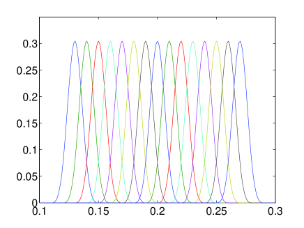
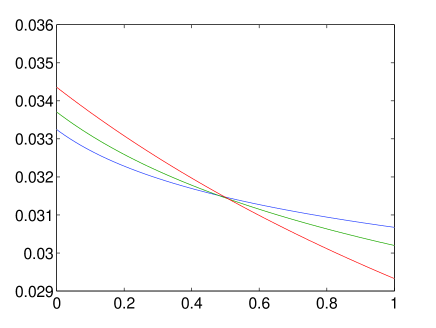
Figure 1: Left graph: cubic B spline functions, in the rage $x\in[0.1,0.3]$, from the set spanning the space of the signal response. Right graph: three of the functions spanning the space of the background.

Randomly taking 30 B-splines $\{B_{\ell_{i}}\}_{i=1}^{30}$ from $B$ we simulate a spectrum by a weighted superposition of such functions, i.e., the response signal is modelled as

$$\langle x|f_{{\cal{V}}}\rangle=f_{\cal{V}}(x)=\sum_{i=1}^{30}c_{\ell_{i}}B_{\ell_{i}}(x),\quad x\in[0,1],$$ (11)

with the coefficients $c_{\ell_{i}}$ randomly chosen from $[0,1]$.

We simulate a background by considering that it belongs to the subspace ${\cal{W}^{\bot}}$ spanned by the set of functions

$$Y=\{y_{j}(x)=(x+0.01j)^{-0.01j},\,x\in[0,1]\}_{j=1}^{50}.$$

A few functions from this set are plotted in the right hand graph of Figure 1 (normalized to unity on $[0,1])$. The background, $g(x)$, is generated by the linear combination

$$\langle x|g\rangle=g(x)=\sum_{j=1}^{50}j^{4}e^{-0.05j}y_{j}(x).$$ (12)

To simulate the data we have perturbed the superposition of $\eqref{sir}$ and $\eqref{bac}$, by ‘very small’ Gaussian errors (of variance up to $0.00001\%$ the value of each data point) and plotted the simulated data in the left hand graph of Figure 2.

This example illustrates well how sensitive to errors the oblique projection is. The subspaces we are dealing with are disjoint: the last five singular values of operator $\hat{U}^{\ast}$ (c.f. (7)) are:

$$0.3277,0.3276,1.0488\times 10^{-4},6.9356\times 10^{-8},2.3367\times 10^{-10},$$

while the first is $\sigma_{1}=1.4493$. The smallest singular value cannot be considered a numerical representation of zero when the calculations are being carried out in double precision arithmetic. Hence, one can assert that the condition ${\cal{V}}\cap{\cal{W}^{\bot}}=\{0\}$ is fulfilled. However, due to the three small singular values the oblique projector along ${\cal{W}^{\bot}}$ onto the whole subspace ${\cal{V}}$ is very unstable, which fails to correctly separate the signals in ${\cal{V}}$ from the background. The result of applying the oblique projector onto the signal of the left hand graph is represented by the broken line in the right hand graph. As can be observed, the projection does not yield the required signal, which is represented by the continuous dark line in the same graph. Now, since the spectrum of singular values has a clear jump (the last three singular values are far from the previous ones) it might seem that one could regularize the projection by truncation of singular values. Nevertheless, such a methodology turns out to be inappropriate for the present problem, as it does not yield the correct separation.

Proposition 2 below analyzes the effect that regularization by truncation of singular values has on the resulting projection.

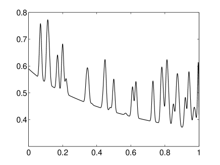
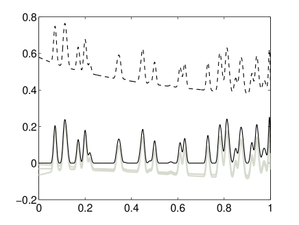
Figure 2: Left graph: signal plus background. Right graph: the dark continuous line corresponds to the signal to be discriminated from the one in the left graph. The broken line corresponds to the approximation resulting from the oblique projection. The three close light lines correspond to the approximations obtained by truncation of one, two, and three singular values.

Proposition 2.

Truncation of the expansion (9) to consider up to $r$ terms, produces an oblique projector along $\tilde{{\cal{W}}}_{r}={\cal{W}^{\bot}}+\tilde{{\cal{W}}}_{0}+\tilde{{\cal{V}}}_{0}$, with $\tilde{{\cal{V}}}_{0}=\text{span}\{|\eta_{i}\rangle\}_{i=r+1}^{N}$ and $\tilde{{\cal{W}}}_{0}=\text{span}\{|\xi_{i}\rangle\}_{i=r+1}^{N}$, onto $\tilde{{\cal{V}}}_{r}=\text{span}\{|\eta_{i}\rangle\}_{i=1}^{r}$.

The proof of this proposition is to be found in Appendix B.

The above example illustrates very clearly the need for nonlinear approaches. We know that a unique and stable solution does exist, since the signal which is to be discriminated from the background actually belongs to a subspace of the given spline space, and the construction of the oblique projectors onto such a subspace is well posed. However, the lack of knowledge about the subspace prevents us from separating the signal components by a linear operation. The greedy approaches that have been proposed for making tractable the search for the unknown subspace proceed in a stepwise manner [3, 4]. Within those approaches, all the effort is focussed on the search for the right subspace for recursively constructing and adapting the vectors $|w_{i}\rangle$ (c.f. (4)). Conceptually, the proposal in [4] implies to assume a priori that none of the system states is populated and uses the available signal to determine which are the populated ones. Here we wish to investigate the outcomes yielded by the converse prior assumption, i.e., by considering a priori that all the states are equally populated and use the available signal to learn which are the non-populated ones.

4 The proposed nonlinear approach

We start by recalling the available strategy for transforming the problem of discriminating the system’s signal response $|f_{\cal{V}}\rangle$ from a given signal $|f\rangle=|f_{\cal{V}}\rangle+|f_{\cal{W}^{\bot}}\rangle$ into the problem of constructing the sparse representation of $|f_{\cal{V}}\rangle$ in ${\cal{V}}$. Let us stress, once again that i) the problem we need to face arises from the ill-posed feature of the oblique projectors onto the whole subspace ${\cal{V}}$ and ii) we work under the hypothesis that there exists an unknown subspace ${{\cal{V}}_{K}}=\text{span}\{{|v_{\ell_{i}}\rangle}\}_{i=1}^{K}\subset{\cal{V}}$, where $\{{\ell_{i}}\}_{i=1}^{K}$ is a set of $K$ unknown indexes such that

$$|f_{{\cal{V}}}\rangle=|f_{{\cal{V}}_{K}}\rangle=\sum_{i=1}^{K}c_{\ell_{i}}|v_{\ell_{i}}\rangle.$$ (13)

Equivalently, (13) can be expressed in the form

$$|f_{{\cal{V}}}\rangle=|f_{{\cal{V}}_{K}}\rangle=\sum_{i=1}^{M}c_{i}|v_{i}\rangle,\,\,\text{with}\,\,c_{i}=0\,\,\text{if}\,\,i\neq{\ell_{j}},\,j=1\ldots,K.$$ (14)

Hence, to find the subspace ${{\cal{V}}_{K}}$ is equivalent to finding the sparse representation of $|f_{{\cal{V}}}\rangle$ in ${{\cal{V}}}$, i.e. a representation given by (14) where only $K$ coefficients are nonzero. However we need to allow for the fact that we do not have access to the signal $|f_{{\cal{V}}}\rangle$ but only to the signal $|f\rangle$. As proposed in [4], we can deal somehow with this lack of information by noticing that by applying the projector $\hat{P}_{{\cal{W}}}$ both sides of (14) we have

$$|f_{\cal{W}}\rangle=|f_{{\cal{W}}_{K}}\rangle=\sum_{i=1}^{M}c_{i}|u_{i}\rangle,$$ (15)

where $|f_{{\cal{W}}_{K}}\rangle=\hat{P}_{{\cal{W}}}|f_{{\cal{V}}_{K}}\rangle$ and $|f_{\cal{W}}\rangle=\hat{P}_{{\cal{W}}}|f\rangle$. Denoting by $\hat{I}_{\SS}$ the identity operator in $\SS$ the projector $\hat{P}_{{\cal{W}}}$ is obtained as $\hat{P}_{{\cal{W}}}=\hat{I}_{\SS}-\hat{P}_{{\cal{W}^{\bot}}}$. Thus, since the subspaces $\SS$ and ${\cal{W}^{\bot}}$ are known, we do have access to the component $|f_{{\cal{W}}}\rangle$. Because the coefficients in (14) and (15) are identical, one can find the sparse representation (14) by finding the sparse representation (15) and using the resulting coefficients in (14).

At this point we begin to differ from the proposal in [4]. While in that publication the problem is tackled by a greedy stepwise search for the indices $\ell_{i},\,i=1,\ldots,K$ in (13), here we take a different route and strive to find the sparse solution of (15) by minimization of the $q-$norm like quantity

$$\||c\rangle\|_{q}^{q}=\sum_{i=1}^{M}|c_{i}|^{q},\quad\text{with}\quad 0<q\leq 1.$$ (16)

The minimization of the $q$-norm^q for determining a sparse solution has been studied in Mathematics and Signal Processing and justified by the following consideration. The problem of finding the sparsest representation of a given model is equivalent to minimization of the zero norm $\|c\rangle\|_{0}$ (or counting measure) which is defined as:

$$\||c\rangle\|_{0}=\sum_{i=1}^{M}|c_{i}|^{0}$$

and therefore is equal to the number of nonzero entries of $|c\rangle$. The minimization of $\||c\rangle\|_{0}$ subject to linear constraints is a classical problem of combinatorial search, which is in general NP-hard [18]. Thus, the minimization of $\sum_{i=1}^{M}|c_{i}|^{q},$ for $0<q\leq 1$ has been considered [6]. However since the minimization of $\sum_{i=1}^{M}|c_{i}|^{q},\,0<q<1$ does not lead to a convex optimization problem, the most popular norm to minimize, when a sparse solution is required, is the 1-norm $\sum_{i=1}^{M}|c_{i}|$. Minimization of the 1-norm is considered the best convex approximant to the minimizer of $\||c\rangle\|_{0}$ [19, 20]. Moreover, it can be efficiently solved by linear programming techniques [19]. Since the problem of signal separation we are considering admits a unique solution, we are not particularly concerned about convexity. Hence we will set up our numerical strategy letting the parameter $q$ take any value in $(0,1]$.

4.1 Managing the constraints

The optimization process we consider is stated as follows: Given the constraints (15) minimize $\sum_{i=1}^{M}|c_{i}|^{q}.$

Now, in general, in order make use of constraints (15) we need a numerical representation of $|f_{\cal{W}}\rangle$, which in practice is obtained by experimental measures. Thus, while restricting considerations to linear measurements we represent them as linear functionals, which, as established by Riesz’ theorem [21], are amenable to representation by inner products with some vectors. Accordingly, we express measures on $|f\rangle$ by the inner products

$$m_{j}=\langle m_{j}|f\rangle,\quad j=1,\ldots,N.$$

The specification of the measurement vectors $|m_{j}\rangle,\,j=1,\ldots,N$ should be given in each particular case. The ones considered here have been chosen in relation to the examples we are presenting. Firstly, to simulate the observed data we suppose that the measures are performed by varying some parameter (e. g. time, wavelength, temperature) that is denoted as the variable ‘$x$’ discretized at the points $x_{j},\,j=1,\ldots,N$ to obtain the measures

$$f_{\cal{W}}(x_{j})=\langle x_{j}|f_{\cal{W}}\rangle,\quad j=1,\ldots,N$$

and the corresponding linear functionals

$$\langle x_{j}|u_{i}\rangle=\langle x_{j}|\hat{P}_{{\cal{W}}}|v_{i}\rangle,,\quad j=1,\ldots,N$$

from the state’s signal responses $|v_{i}\rangle,\,i=1,\ldots,M$. While the functionals $\langle x_{j}|u_{i}\rangle$ are modeled according to physical considerations, the values $f_{\cal{W}}(x_{j})$ are experimental data, thereby affected by errors. We then use the notation $f^{o}_{\cal{W}}(x_{j}),\,j=1,\ldots,N$ to indicate the observations of $f_{\cal{W}}(x_{j}),\,j=1,\ldots,N$. Consequently, rather than reproducing the data $f^{o}_{\cal{W}}(x_{j}),\,j=1,\ldots,N$ we request that the model given by the r.h.s. of (15) satisfies the restriction

$$\sum_{j=1}^{N}(f^{o}_{\cal{W}}(x_{j})-f_{\cal{W}}(x_{j}))^{2}\leq\delta,$$ (17)

$\delta$ accounting for the data’s error. The stated optimization process subjected to this constraint is numerically difficult to realize. Nevertheless, we show here that the available information can be handled so as to successfully achieve the discrimination of signal components, even when the data errors are significant. For this we make use of an idea we had introduced much earlier, in [22], and applied in [23]: Replacing $f_{\cal{W}}(x_{j})$ by (15), the condition of minimal square distance $\sum_{j=1}^{N}(f^{o}_{\cal{W}}(x_{j})-f_{\cal{W}}(x_{j}))^{2}$ leads to the so called normal equations:

$$\langle u_{n}|f_{W}^{o}\rangle=\sum_{i=1}^{M}c_{i}\langle u_{n}|u_{i}\rangle,\quad n=1\ldots,M.$$ (18)

Of course, since we are concerned with ill posed problems we cannot use all these equations to find the coefficients $c_{i},\,i=1,\ldots,M$. However, as proposed in [22], we could use ‘some’ of these equations as constraints of our optimization process. The number of such equations being the necessary to reach the condition (17).

We have then transformed the original problem into the one of minimizing (16) subject to a number of equations selected from $\eqref{noreq}$, the $\ell_{n}$-th$,\,n=1\ldots,r$ ones say. We leave for the moment the restrictions $c_{i}\geq 0,\,i=1,\ldots,M$. We should worry about them only if they were not satisfied.

In line with [22] we select the subset of equations (18) in an iterative fashion. We start by the initial estimation $c_{i}=C,\,i=1,\ldots,M$, where the constant $C$ is determined by minimizing the distant between the model and the data. Thus,

$$C=\frac{\sum_{n=1}^{M}\langle u_{n}|f^{o}_{\cal{W}}\rangle}{\sum_{i=1}^{M}\sum_{n=1}^{M}\langle u_{i}|u_{n}\rangle}.$$ (19)

With this initial estimation we ‘predict’ the normal equations (18) and select as our first constraint the worst predicted by the initial solution, let this equation be the $\ell_{1}$-th one. We then minimize (16) subject to the constraint

$$\langle u_{\ell_{1}}|f_{\cal{W}}^{o}\rangle=\sum_{i=1}^{M}c_{i}\langle u_{{\ell_{1}}}|u_{i}\rangle,$$ (20)

and indicate the resulting coefficients as $c_{i}^{(1)},\,i=1,\ldots,M$. With these coefficients we predict equations (18) and select the worst predicted as a new constraint to obtain $c_{i}^{(2)},\,i=1,\ldots,M$ and so on. The iterative process is stopped when the condition (17) is reached.

The reader may be aware that the proposed strategy involves highly nonlinear equations and in many situations the number of necessary constraints is large enough to generate a troublesome numerical task. However, we have been able to solve the simulation of the next section (comprising up to 57 constraints) by recourse to the method for minimization of the $(q$-norm)^q published in [6]. Such an iterative method, called FOCal Underdetermined System Solver (FOCUSS) in that publication, is straightforward implementable. It evolves by computation of pseudoinverse matrices, which under the given hypothesis of our problem, and within our recursive strategy for feeding the constraints, are guaranteed to be numerically stable (for a detailed explanation of the method see [6]).

4.2 Numerical Simulation

We test the proposed approach, first on the simulation of Example 1 of Section 3, and then extend that simulation to consider a more realistic level of uncertainty in the data. Let us remark that the signal is meant to represent an emission spectrum consisting of the superposition of spectral lines (modeled by B-spline functions of support 0.04) which are centered at the positions $(n-1)\Delta,\,n=0,\ldots,102$, with $\Delta=0.01$. Since the errors in the data in Example 1 are not significant, the procedure outlined in the previous section accurately recovers the spectrum from the background, with any positive value of the $q$-parameter less than or equal to one. The result (coinciding with the theoretical one) is shown in the right hand top graph of Figure 3.

Now we transform the example into a more realistic situation by adding larger errors to the data. In this case, the data set is perturbed by Gaussian errors of variance up to $1\%$ of each data point. Such a piece of data is plotted in the left middle graph of Figure 3 and the spectrum extracted by the the proposed approach is represented by the broken line in the right middle graph of Figure 3, which is difficult to differentiate from the theoretical one (continuous line).

Finally we increase the data’s error up to $3\%$ of each data point (left bottom graph of Figure 3) and, in spite of the perceived significant distortion of the signal, we could still recover a spectrum which, as shown by the broken line in the right bottom graph of Figure 3, is a fairly good approximation of the true one (continuous line).

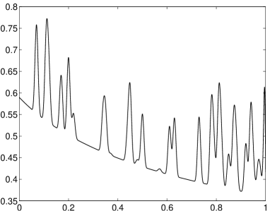
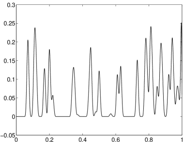
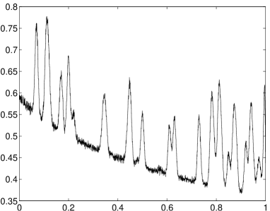
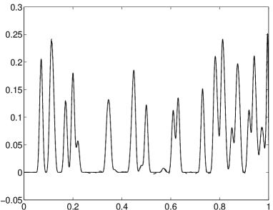
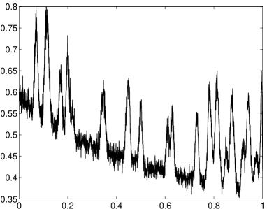
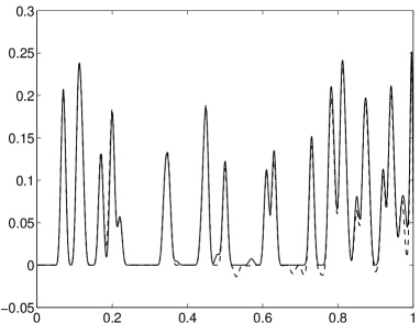
Figure 3: Top left graph: signal plus background generated as described in Example 1 of Section 3. Top right graph: Recovered system’ signal response, which coincides with the true one. Middle left graph: signal of Example 1 distorted by Gaussian errors of variance up to $1\%$ of each data value. Middle right graph: the broken line represents the approximation of the system’ signal response yielded by the proposed approach. The continuous line represents the true signal. Bottom graphs: Same description as in the previous graphs but the data distorted by Gaussian errors of variance up to $3\%$ of each data value.

We have repeated the experiment for different realization of the errors (with the same variance) and the results remained essentially equivalent. Moreover, we have considered other realizations of the experiment by drawing different spectra through the process described in Section 3. By observing the outcomes of a number the different realizations we can assert that the quality of the results shown in Figure 3 is a fair representation of those obtained for different spectra. Variation of the $q$-value did not produce significant changes. The results of Figure 3 were obtained for the value $q=0.8$. The number of equations that were necessary to use in order to reach the stopping criterion for the different level of error were: $K=57$ for the data in the top graph, $K=51$ for the data in the middle graph and $K=43$ for the bottom graph.

It is appropriate to stress once more that for small level of errors the solution of this example is unique. The numerical experiment illustrates the fact that, for the degree of sparsity being considered (out to 103 states only 30 are populated) the solution can be reached by the whole range of $q$ values in $(0,1]$. This is so because for all $q$ in the range $(0,1]$ the number of constraints which are needed to obtain the solution is still small enough to yield a well posed problem. Let us stress further that, we have not made explicit used of the constraints $c_{i}\geq 0,\,i=1,\ldots,M$ but look for the solution by minimization of the quantity $\sum_{i=1}^{M}|c_{i}|^{q}$, which is non-extensive for all $q$-values.

5 Conclusions

The problem of discriminating information produced by phenomena of different nature has been addressed through a non-extensive nonlinear approach. The proposed framework is founded on the minimization of a $q-$norm like quantity. It is appropriate to remark that our main concern was to realize the discrimination of information components in cases admitting a unique theoretical solution. The problem was transformed into an underdetermined linear one, due to the numerical instability of the concomitant full rank problem. The resulting approach has been tested by recourse to a numerical example which cannot be handled by linear techniques (even for unrealistically high quality data). A detailed analysis of the limitation affecting the linear technique has been provided. The nonlinear approach presented here was shown to be capable of overcoming those limitations. It has correctly realized the required task, even for data distorted by significant random errors. We are aware that further studies may be in order and we are confident that the results presented here will motivate future works.

References

- [1] R. Behrens, L. Scharf, Signal processing applications of oblique projection operators, IEEE Transactions on Signal Processing 42 (1994) 1413–1424.
- [2] L. Rebollo-Neira, Constructive updating/downdating of oblique projectors: a generalization of the Gram–Schmidt process, Journal of Physics A: Mathematical and Theoretical 40 (2007) 6381–6394.
- [3] L. Rebollo-Neira, Oblique matching pursuit, IEEE Signal Processing Letters 14 (10) (2007) 703–706.
- [4] L. Rebollo-Neira, Measurements design and phenomena discrimination, J. Phys. A: Math. Theor. 42 (2009) 165210.
- [5] M. V. Wickerhauser, Adapted Wavelet Analysis from Theory to Software, AK Peters, Ltd (2004).
- [6] B.D. Rao and K. Kreutz-Delgado, An Affine Scaling Methodology for Best Basis Selection, IEEE Trans. Sig. Proc. 47 (1999) 187–200.
- [7] C. Tsallis, Possible generalization of Boltzmann-Gibbs statistics, J. Stat. Phys., 52, (1988) 479.
- [8] C. Tsallis Introduction to nonextensive statistical mechanics, Springer-Verlag, NY, (2009).
- [9] A. R. Plastino, A. Plastino, Tsallis Stellar Polytropes and Tsallis’ entropy, Physics Letters A, 174 (1993) 834–386.
- [10] A. R. Plastino, A. Plastino, Tsallis Entropy, Erhenfest Theorem and Information Theory, Physics Letters A, 177 (1993) 177–179.
- [11] B. R. La Cour, W. C. Schieve, Tsallis maximum entropy principle and the law of large numbers, Phys. Rev. E 62 (2000) 7494–7496.
- [12] S. Abe, Y. Okamoto, Nonextensive Statistical Mechanics and Its Applications Series: Lecture Notes in Physics , Vol. 560 Springer-Verlag, NY (2001).
- [13] Y. Eldar, Sampling with arbitrary sampling and reconstruction spaces and oblique dual frame vectors, Journal of Fourier Analysis and Applications 9 (2003) 77–96.
- [14] G. Corach, A. Maestripieri, D Stojanoff, A Classification of Projectors, Banach Center Publ. 67 (2005), 145–160.
- [15] G. Corach, A. Maestripieri, D Stojanoff, Projections in operators ranges, Proc. Amer. Math. Soc. 134 (2005), no 3, 765–788.
- [16] L. Schumaker, Spline Functions: Basic Theory, Wiley, New York, 1981.
- [17] M. Andrle, L. Rebollo-Neira, Cardinal B-spline dictionaries on a compact interval, Applied and Computational Harmonic Analysis 18 (2005) 336–346.
- [18] B.K. Natarajan, Sparse approximate solutions to linear systems, SIAM J. Comput. 24 (1995) 227–234.
- [19] S.S. Chen and D.L. Donoho and M.A. Saunders, Atomic Decomposition by Basis Pursuit, SIAM Journal on Scientific Computing, 20 (1998) 33–61.
- [20] S.S. Chen and D.L. Donoho and M.A. Saunders, Atomic Decomposition by Basis Pursuit, SIAM Rev. 43 (2001) 129–156.
- [21] M. Reed, B. Simon, Functional Analysis, Academic Press, London, 1980.
- [22] L. Rebollo-Neira, A. Constantinides, A. Plastino, F. Zyserman, A. Alvarez, R. Bonetto, H. Viturro, Statistical inference, state distribution, and noisy data, Physica A 198 (1993) 514–537
- [23] L. Rebollo-Neira, A. G. Constantinides, A. Plastino, A. Alvarez, Bonetto, M. Iñiguez Rodriguez, Statistical analysis of a mixed-layer x-ray diffraction peak, Journal of Physics, 30, 17 (1997) 2462–2469.