Adaptive non-uniform B-spline dictionaries on a compact interval

Abstract

Non-uniform B-spline dictionaries on a compact interval are discussed. For each given partition, dictionaries of B-spline functions for the corresponding spline space are constructed. It is asserted that, by dividing the given partition into subpartitions and joining together the bases for the concomitant subspaces, slightly redundant dictionaries of B-splines functions are obtained. Such dictionaries are proved to span the spline space associated to the given partition. The proposed construction is shown to be potentially useful for the purpose of sparse signal representation. With that goal in mind, spline spaces specially adapted to produce a sparse representation of a given signal are considered.

1 Introduction

A representation in the form of a linear superposition of elements of a vector space is said to be sparse if the number of elements in the superposition is small, in comparison to the dimension of the corresponding space. The interest for sparse representations has enormously increased the last few years, in large part due to their convenience for signal processing techniques and the results produced by the theory of Compressed Sensing with regard to the reconstruction of sparse signals from non-adaptive measurements [1, 2, 3, 4, 5]. Furthermore, the classical problem of expressing a signal as a linear superposition of elements taken from an orthogonal basis has been extended to consider the problem of expressing a signal as a linear superposition of elements, called atoms, taken from a redundant set, called dictionary [6]. The corresponding signal approximation in terms of highly correlated atoms is said to be highly nonlinear and has been proved relevant to signal processing applications. Moreover, a formal mathematical setting for highly nonlinear approximations is being developed. As a small sample of relevant literature let us mention [7, 8, 9].

In regard to sparse approximations there are two main problems to be looked at; one is in relation to the design of suitable algorithms for finding the sparse approximation, and other the construction of the dictionaries endowing the approximation with the property of sparsity. In this communication we consider the sparse representation matter for the large class of signals which are amenable to satisfactory approximation in spline spaces [10, 11]. Given a signal, we have the double goal of a) finding a spline space for approximating the signal and b) constructing those dictionaries for the space which are capable of providing a sparse representation of such a signal. In order to achieve both aims we first discuss the construction of dictionaries of B-spline functions for non-uniform partitions, because the usual choice, the B-spline basis for the space, is not expected to yield sparse representations.

In a previous publication [12] a prescription for constructing B-spline dictionaries on the compact interval is advised by restricting considerations to uniform partitions (cardinal spline spaces). Since our aim entails to relax this restriction, we are forced to look at the problem from a different perspective. Here we divide the partition into subpartitions and construct the dictionary by joining together the bases for the subspaces associated to each subpartition. The resulting dictionary is proved to span the spline space for the given non-uniform partition. Consequently, the uniform case considered in [12] arises as a particular case of this general construction. The capability of the proposed nonuniform dictionaries to produce sparse representations is illustrated by a number of examples.

The letter is organized as follows: Section 2 introduces splines spaces and gives the necessary definitions. The property of splines spaces which provides us with the foundations for the construction of the proposed dictionaries is proven in this section (c.f. Theorem 2). For a fixed partition, the actual constructions of non-uniform B-spline dictionaries is discussed in Section 3. Section 4 addresses the problem of finding the appropriate partition giving rise to the spline space suitable for approximating a given signal. In the same section a number of examples are presented, which illustrate an important feature of dictionaries for the adapted spaces. Namely, they may render a very significant gain in the sparseness of the representation of those signals which are well approximated in the corresponding space. The conclusions are drawn in Section 5.

2 Background and notations

We refer to the fundamental books [13, 14, 15] for a complete treatment of splines. Here we simply introduce the adopted notation and the basic definitions which are needed for presenting our results.

Definition 1.

Given a finite closed interval $[c,d]$ we define a partition of $[c,d]$ as the finite set of points

$$\Delta:=\{x_{i}\}_{i=0}^{N+1},N\in\mathbb{N},\,\,\text{such that}\,\,c=x_{0}<x_{1}<\cdots<x_{N}<x_{N+1}=d.$$ (1)

We further define $N$ subintervals $I_{i},i=0,\dots,N$ as: $I_{i}=[x_{i},x_{i+1}),i=0,\dots,N-1$ and $I_{N}=[x_{N},x_{N+1}]$.

Definition 2.

Let $\Pi_{m}$ be the space of polynomials of degree smaller or equal to $m\in\mathbb{N}_{0}=\mathbb{N}\cup\{0\}$. Let $m$ be a positive integer and define

$$S_{m}(\Delta)=\{f\in C^{m-2}[c,d]\ :\ f|_{I_{i}}\in\Pi_{m-1},i=0,\dots,N\},$$ (2)

where $f|_{I_{i}}$ indicates the restriction of the function $f$ on the interval ${I_{i}}$.

The standard result established by the next theorem is essential for our purpose.

Theorem 1.

([13], pp.111) Let

$$\Delta:=\{x_{i}\}_{i=0}^{N+1},\,\,N\in\mathbb{N},\,\,\text{such that}\,\,c=x_{0}<x_{1}<\cdots<x_{N}<x_{N+1}=d.$$ (3)

Then

$$S_{m}(\Delta)\,\,=\,\,{\rm span}\{1,x,\ldots,x^{m-1},(x-x_{i})^{m-1}_{+},i=1,\ldots,N\},$$

where $(x-x_{i})^{m-1}_{+}=(x-x_{i})^{m-1}$ for $x-x_{i}>0$ and $0$ otherwise.

We are now ready to prove the theorem from which our proposal will naturally arise.

Theorem 2.

Suppose that $\Delta_{1}$ and $\Delta_{2}$ are two partitions of $[c,d]$. It holds to be true that

$$S_{m}(\Delta_{1})+S_{m}(\Delta_{2})=S_{m}(\Delta_{1}\cup\Delta_{2}).$$

Proof.

It stems from Theorem 1 and the basic result of linear algebra establishing that for $A_{1}$ and $A_{2}$ two sets such that $S_{1}=\operatorname{span}\{A_{1}\}$ and $S_{2}=\operatorname{span}\{A_{2}\}$, one has $S_{1}+S_{2}=\operatorname{span}\{A_{1}\cup A_{2}\}$.

Certainly, from Theorem 1 and for

$$A_{1}:=\{1,x,\ldots,x^{m-1},(x-x_{i})^{m-1}_{+},x_{i}\in\Delta_{1}\}\quad{\text{and}}\quad A_{2}:=\{1,x,\ldots,x^{m-1},(x-x_{i})^{m-1}_{+},x_{i}\in\Delta_{2}\}$$

we have: $S_{m}(\Delta_{1})=\operatorname{span}\{A_{1}\}$,  $S_{m}(\Delta_{2})=\operatorname{span}\{A_{2}\}$. Hence

$$S_{m}(\Delta_{1})+S_{m}(\Delta_{2}) = \operatorname{span}\{A_{1}\cup A_{2}\}$$

$$= \operatorname{span}\{1,x,\ldots,x^{m-1},(x-x_{i})^{m-1}_{+},x_{i}\in\Delta_{1}\cup\Delta_{2}\}$$

so that, using Theorem 1 on the right hand side, the proof is concluded. ∎

The next corollary is a direct consequence of the above theorem.

Corollary 1.

Suppose that $\Delta_{j},j=1,\ldots,n$ are partitions of $[c,d]$. Then

$$S_{m}(\Delta_{1})+\cdots+S_{m}(\Delta_{n})\,\,=\,\,S_{m}(\cup_{j=1}^{n}\Delta_{j}).$$

3 Building B-spline dictionaries

Let us start by recalling that an extended partition with single inner knots associated with $S_{m}(\Delta)$ is a set $\tilde{\Delta}=\{y_{i}\}_{i=1}^{2m+N}$ such that

$$y_{m+i}=x_{i},\,\,i=1,\ldots,N,\,\,x_{1}<\cdots<x_{N}$$

and the first and last $m$ points $y_{1}\leq\cdots\leq y_{m}\leq c,\quad d\leq y_{m+N+1}\leq\cdots\leq y_{2m+N}$ can be arbitrarily chosen.

With each fixed extended partition $\tilde{\Delta}$ there is associated a unique B-spline basis for $S_{m}(\Delta)$, that we denote as $\{B_{m,j}\}_{j=1}^{m+N}$. The B-spline $B_{m,j}$ can be defined by the recursive formulae [13]:

$$B_{1,j}(x) = \begin{cases}1,&t_{j}\leq x<t_{j+1},\\ 0,&{\rm otherwise,}\end{cases}$$

$$B_{m,j}(x) = \frac{x-y_{j}}{y_{j+m-1}-y_{j}}B_{m-1,j}(x)+\frac{y_{j+m}-x}{y_{j+m}-y_{j+1}}B_{m-1,j+1}(x).$$

The following theorem paves the way for the construction of dictionaries for $S_{m}(\Delta)$. We use the symbol $\#$ to indicate the cardinality of a set.

Theorem 3.

Let $\Delta_{j},\,j=1,\ldots,n$ be partitions of $[c,d]$ and $\Delta=\cup_{j=1}^{n}\Delta_{j}$. We denote the B-spline basis for $S_{m}(\Delta_{j})$ as $\{B_{m,k}^{(j)}:k=1,\ldots,m+\#\Delta_{j}\}$. Accordingly, a dictionary, ${\mathcal{D}}_{m}(\Delta:\cup_{j=1}^{n}\Delta_{j})$, for $S_{m}(\Delta)$ can be constructed as

$${\mathcal{D}}_{m}(\Delta:\cup_{j=1}^{n}\Delta_{j})\,\,:=\,\,\cup_{j=1}^{n}\{B_{m,k}^{(j)}:k=1,\ldots,m+\#\Delta_{j}\},$$

so as to satisfy

$${\rm span}\{{\mathcal{D}}_{m}(\Delta:\cup_{j=1}^{n}\Delta_{j})\}\,\,=\,\,S_{m}(\Delta).$$

When $n=1$, ${\mathcal{D}}_{m}(\Delta:\Delta_{1})$ is reduced to the B-spline basis of $S_{m}(\Delta)$.

Proof.

It immediately follows from Corollary 1. Indeed,

$${\rm span}\{{\mathcal{D}}_{m}(\Delta:\cup_{j=1}^{n}\Delta_{j})\} = {\rm span}\{\cup_{j=1}^{n}\{B_{m,k}^{(j)}:k=1,\ldots,m+\#\Delta_{j}\}\}$$

$$= S_{m}(\Delta_{1})+\cdots+S_{m}(\Delta_{1})=S_{m}(\cup_{j=1}^{n}\Delta_{j})=S_{m}(\Delta).$$

∎

Remark 1.

Note that the number of functions in the above defined dictionary is equal to $n\cdot m+\sum_{j=1}^{n}\#\Delta_{j}$, which is larger than $\dim S_{m}(\Delta)=m+\#\Delta$. Hence, excluding the trivial case $n=1$, the dictionary constitutes a redundant dictionary for $S_{m}(\Delta)$.

According to Theorem 3, to build a dictionary for $S_{m}(\Delta)$ we need to choose $n$-subpartitions $\Delta_{j}\in\Delta$ such that $\cup_{j=1}^{n}\Delta_{j}=\Delta$. This gives a great deal of freedom for the actual construction of a non-uniform B-spline dictionary. Fig. 1 shows some examples which are produced by generating a random partition of $[0,4]$ with 6 interior knots. From an arbitrary partition

$$\Delta\,\,:=\,\,\{0=x_{0}<x_{1}<\cdots<x_{6}<x_{7}=4\},$$

we generate two subpartitions as

$$\Delta_{1}\,\,:=\,\,\{0=x_{0}<x_{1}<x_{3}<x_{5}<x_{7}=4\},\quad\Delta_{2}\,\,:=\,\,\{0=x_{0}<x_{2}<x_{4}<x_{6}<x_{7}=4\}$$

and join together the B-spline basis for $\Delta_{1}$ (light lines in the right graphs of Fig. 1) and $\Delta_{2}$ (dark lines in the same graphs)

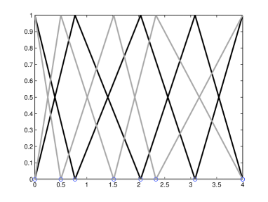
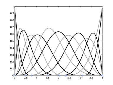
Figure 1: Examples of bases (graphs on the left) and the corresponding dictionaries (right graphs) for a random partition $\Delta$ consisting of 6 interior knots. The top graphs correspond to linear B-splines ($m=2$). The bottom graphs involve cubic B-splines ($m=4$). The top left graph depicts the B-spline basis for $S_{2}(\Delta)$ whereas the right one depicts the B-spline dictionary ${\mathcal{D}}_{2}(\Delta:\Delta_{1}\cup\Delta_{2})$ arising by merging the B-spline basis for $S_{2}(\Delta_{1})$ and for $S_{2}(\Delta_{2})$ (light and dark lines, respectively). The bottom graphs have the same description as the top graphs, but correspond to $S_{4}(\Delta)$ and ${\mathcal{D}}_{4}(\Delta:\Delta_{1}\cup\Delta_{2}).$

Remark 2.

As should be expected, the cardinal B-spline dictionaries introduced in [12] arise here as particular cases of the proposed construction. In order to show this we use $\Delta_{b}$ to denote an equidistant partition of $[c,d]$ with distance $b$ between adjacent points such that $(d-c)/b\in\mathbb{Z}$, i.e., $\Delta_{b}$ is composed by the inner knots $x_{j}=c+jb,\,j=1,\ldots,(d-c)/b$. We also consider the partition $\Delta_{j_{0},b^{\prime}}$ with knots $x_{j}=c+j_{0}b+jb^{\prime}$, where $b^{\prime}/b\in\mathbb{Z}$ and $j_{0}$ is a fixed integer in $[0,b^{\prime}/b-1]$. Since $\cup_{j_{0}=0}^{{b^{\prime}/b-1}}\Delta_{j_{0},b^{\prime}}=\Delta_{b}$, we can build a dictionary as

$${\mathcal{D}}_{m}(\Delta_{b}:\cup_{j=0}^{b^{\prime}/b-1}\Delta_{j,b^{\prime}})\,\,=\,\,\cup_{j_{0}=0}^{{b^{\prime}/b-1}}\{B_{m,k}^{(j_{0})}:k=1,\ldots,m+\#\Delta_{j_{0},b^{\prime}}\},$$

where $B_{m,k}^{(j_{0})},k=1,\ldots,m+\#\Delta_{j_{0},b^{\prime}}$ is the cardinal B-spline basis for the subspace determined by the partition $\Delta_{j_{0},b^{\prime}}$. This yields a cardinal B-spline dictionary as proposed in [12].

4 Application to sparse signal representation

Given a signal, $f$ say, we address now the issue of determining a partition $\Delta$, and sub-partitions $\Delta_{j},j=1,\ldots,n$, such that: a) $\cup_{j=1}^{n}\Delta_{j}=\Delta$ and b) the partitions are suitable for generating a sparse representation of the signal in hand. As a first step we propose to tailor the partition to the signal $f$ by setting $\Delta$ taking into account the critical points of the curvature function of the signal, i.e.,

$$T\,\,:=\,\,\{t:\left(\frac{f^{\prime\prime}}{(1-f^{\prime 2})^{3/2}}\right)^{\prime}(t)=0\}.$$

Usually the entries in $T$ are choosen as the initial knots of $\Delta$. In order to obtain more knots we apply subdivision between consecutive knots in $T$ thereby obtaining a partition $\Delta$ with the decided number of knots.

Because most signals are processed with digital computers, one normally has to deal with a numerical representation of a signal in the form of sampling points. Thus, another problem to be addressed is how to compute the entries in $T$ from the sequence of points $f(kh),k=1,\ldots,n$, where $h$ is the step length in the discretization. The algorithm below outlines a procedure for accomplishing the task.

  Input: the interval $[c,d]$, the discrete signal $f(c+kh),k=0,\ldots,n$, the subdivision level $l$.

  Output: The partition $\Delta$.

  $\Delta=\{\}$

  for  $k=2:n-3$ do

     for $t=0:2$ do

        $df=(f((k+t+1)h)-f((k+t)h))/h$

        $ddf=(f((k+t+1)h)+f((k+t-1)h))-2f((k+t)h))/h^{2}$

        $c_{t}=ddf/(1-df^{2})^{3/2}$

     end for

     if $|c_{0}|<|c_{1}|$ and $|c_{1}|>|c_{2}|$ then

        $\Delta=\Delta\cup\{c+(k+1)h\}$

     end if

  end for

  Set $N\,\,=\,\,\#\Delta$

  Set $\Delta\,\,=\,\,\Delta\cup\{c,d\}$

  Sort the entries in $\Delta$:

$$c=x_{0}<x_{1}<\cdots<x_{N+1}=d$$

  for  $k=0:N$ do

     $\Delta=\Delta\cup\{x_{k}+t(x_{k+1}-x_{k})/l:t=1,\ldots,l-1\}$

  end for

Algorithm 1 Computing the partition $\Delta$: $T(f,l)$.

According to Theorem 3, in order to build a dictionary for $S_{m}(\Delta)$ we need to choose $n$-subpartitions $\Delta_{j}\in\Delta$ such that $\cup_{j=1}^{n}\Delta_{j}=\Delta$. As an example we suggest a simple method for producing $n$-subpartitions $\Delta_{j}\in\Delta$, which is used in the numerical simulations of the next section. Considering the partition $\Delta=\{x_{0},x_{1},\ldots,x_{N+1}\}$ such that $c=x_{0}<x_{1}<\cdots<x_{N+1}=d$, for each integer $j$ in $[1,n]$ we set

$$\Delta_{j}\,\,:=\,\,\{c,d\}\cup\{x_{k}:k\in[1,N]\mbox{ and }k\!\!\mod n=j-1\},$$

e.g. if $N=10$ and $n=3$, we have $\Delta_{1}\,\,=\,\,\{c,x_{3},x_{6},x_{9},d\},\,\,\Delta_{2}\,\,=\,\,\{c,x_{1},x_{4},x_{7},x_{10},d\}$     $\Delta_{3}\,\,=\,\,\{c,x_{2},x_{5},x_{8},d\}.$

It is easy to see that the above defined partitions satisfy $\cup_{j=1}^{n}\Delta_{j}=\Delta$.

4.1 Numerical examples

We produce here three examples illustrating the potentiality of the proposed dictionaries for achieving sparse representations by nonlinear techniques. The signal we consider are the following:

• A chirp signal, $f_{1}=\cos(2\pi x^{2})$, $x\in[0,8],$ plotted in the top left of Fig. 1.

• A seismic signal $f_{2}$ plotted in the top right graph of Fig. 1. This signal was taken from the WaveLab802 Toolbox. It is acknowledged there that the signal is distributed throughout the seismic industry as a test dataset.

• A cosine function of random phase $f_{3}=\cos(8\pi x+\phi(x)),$ where $\phi(x)$ is the piecewise constant function depicted in the bottom right of Fig. 1. The left graph corresponds to the signal.

Figure 2: Chirp signal $f_{1}=\cos(2\pi x^{2})$ (top left). Seismic signal $f_{2}$ (top right). Cosine signal $f_{3}=\cos(8\pi x+\phi(x))$ (bottom left) for the randomly generate phase $\phi(x)$ plotted in the bottom right graph. The broken lines, indistinguishable from the continue lines representing test signals, are the resulting approximations up to error’s norm ${\rm{tol}}_{i}=0.01||f_{i}||,\,i=1,2,3$.

The three signals are to be approximated up to a tolerance ${\rm{tol}}_{i}=0.01||f_{i}||,\,i=1,2,3$ for the norm of the approximation’s error.

We deal with the chirp signal $f_{1}$ on the interval $[0,8]$, by discretizing it into $L=2049$ samples and applying Algorithm 1 to produce the partition $\Delta=T(f_{1},9)$. The resulting number of knots is $1162$, which is enough to approximate the signal, by a cubic B-spline basis for the space, within the above specified precision ${\rm{tol}_{1}}$. A dictionary ${\mathcal{D}}_{4}(\Delta:\cup_{j=1}^{10}\Delta_{j})$ for the identical space is constructed by considering 10 subpartitions, which yield $N_{1}=1200$ functions.

The signal $f_{2}$ is a piece of $L=513$ data. A partition of cardinality $511$ is obtained as $\Delta=T(f_{1},8)$ and the dictionary of cubic splines we have used arises by considering $3$ subpartitions, which yields a dictionary ${\mathcal{D}}_{4}(\Delta:\cup_{j=1}^{3}\Delta_{j})$ of cardinality $N_{2}=521$.

The signal $f_{3}$ is discretized into $L=2049$ samples. The partition $\Delta=T(f_{1},43)$ produces $732$ knots. Using $26$ subpartitions we build a dictionary ${\mathcal{D}}_{2}(\Delta:\cup_{j=1}^{26}\Delta_{j})$ of $N_{3}=782$ linear B-spline functions.

Denoting by $\alpha^{i}_{n},\,n=1,\ldots,N_{i}$ the atoms of the $i$th-dictionary, we look now for the subsets of indices $\Gamma_{i},\,i=1,2,3$ of cardinality $K_{i},\,i=1,2,3$ providing us with a sparse representation of the signals. In other words, we are interested in the approximations

$$f_{i}^{K_{i}} = \sum_{n\in\Gamma_{i}}c_{n}^{i}\alpha^{i}_{n},\quad i=1,2,3,$$

such that $||f_{i}^{K_{i}}-f_{i}||\leq{\rm{tol}}_{i},\ i=1,2,3,$ and the values $K_{i},\,i=1,2,3$ are satisfactory small for the approximation to be considered sparse. Since the problem of finding the sparsest solution is intractable, for all the signals we look for a satisfactory sparse representation using the same greedy strategy, which evolves by selecting atoms through stepwise minimization of the residual error as follows.

i)The atoms are selected one by one according to the Optimized Orthogonal Matching Pursuit (OOMP) method [16] until the above defined tolerance for the norm of the residual error is reached.

ii)The previous approximation is improved, without greatly increasing the computational cost, by a ‘swapping refinement’ which at each step interchanges one atom of the atomic decomposition with a dictionary atom, provided that the operation decreases the norm of the residual error[17].

iii)A Backward-Optimized Orthogonal Matching Pursuit (BOOMP) method [18] is applied to disregard some coefficients of the atomic decomposition, in order to produce an approximation up to the error of stage i). The last two steps are repeated until no further swapping is possible.

Let us stress that, if steps ii) and iii) can be executed at least once, the above strategy guarantees an improvement upon the results of OOMP. The gain is with respect to the number of atoms involved in the approximation for the given error’s norm.

The described technique is applied to all the non-orthogonal dictionaries we have considered for comparison with the proposed approach. The results are shown in Table 1. In the first column we place the dictionaries to be compared. These are: 1) the spline basis for the space adapted to the corresponding signal, as proposed in Sec 4. As already mentioned, for signals $f_{1}$ and $f_{2}$ we use cubic B-splines and for signal $f_{3}$ the linear one. 2) The dictionary for the identical spaces consisting of functions of larger support. 3) The orthogonal cosine bases used by the discrete cosine transform (dct). 4) The semi-orthogonal cardinal Chui-Wang spline wavelet basis [19] and 5) the Chui-Wang cardinal spline dictionary for the same space [20]. For signals $f_{1}$ and $f_{2}$ we use cubic spline wavelets and for signal $f_{3}$ linear spline wavelets.

Table 1: Comparison of sparsity performance achieved by selecting atoms from the non-uniform bases and dictionaries for adapted spline space (1st and 2nd rows), dft (3rd row), cardinal wavelet bases and dictionaries (4th and 5th rows).

Dictionaries	$K^{1}$ (signal $f_{1}$)	$K^{2}$ (signal $f_{2}$)	$K^{3}$ (signal $f_{3}$)
Non-uniform spline basis	1097	322	529
Non-uniform spline dictionary	173	129	80
Discreet cosine transform	263	208	669
Cardinal Chui-Wang wavelet basis	246	201	97
Cardinal Chui-Wang wavelet dictionary	174	112	92

The last three columns of Table 1 display the number of atoms involved in the atomic decomposition for each test signal and for each dictionary. These numbers clearly show a remarkable performance of the approximation produced by the proposed non-uniform B-spline dictionaries. Notice that whilst the non-uniform spline space is adapted to the corresponding signal, only the dictionary for the space achieves the sparse representation. Moreover the performance is superior to that of the Chui-Wang spline wavelet basis [19] even for signal $f_{3}$, which was specially selected because, due to the abrupt edges delimiting the smooth lines, is very appropriate to be approximated by wavelets. It is also worth stressing that for signal $f_{1}$ and $f_{2}$ the performance is similar to the cardinal Chui-Wang dictionary, which is known to render a very good representation for these signals [20]. However, whilst the Chui-Wang cardinal spline wavelet dictionaries introduced in [20] are significantly redundant with respect to the corresponding basis (about twice as larger) the non-uniform B-spline dictionaries introduced here contain a few more functions than the basis. Nevertheless, as the examples of this section indicate, the improvement in the sparseness of the approximation a dictionary may yield with respect to the B-spline basis is enormous. Still there is the issue of establishing how to decide on the number of subpartitions to be considered. For these numerical examples the number of subpartitions was fixed as the one producing the best result when allowing the number of subpartitions to vary within some range. It was observed that only for signal $f_{2}$ the optimum number of subpartitions produced results significantly better that all other values. Conversely, from signals $f_{1}$ and $f_{3}$ some variations from the optimum number of subpartitions still produce comparable results.

5 Conclusions

Non-uniform B-spline dictionaries for adapted spline spaces have been introduced. The proposed dictionaries are built by dividing a given partition into subpartitions and merging the basis for the concomitant subspaces. The dictionary functions are characterized by having broader support than the basis functions for the identical space. The uniform B-spline dictionaries proposed in [12] readily arise here as a particular case.

The capability of the non-uniform B-spline dictionaries to produce sparse signal representation has been illustrated by recourse to numerical simulations. Thus, we feel confident that a number of applications could benefit from this construction, e.g., we believe it could also be useful in Computer-Aided Geometry Design (CAGD), for reducing control points and for finding sparse knot sets of B-spline curves [21, 22, 23].

Acknowledgements

This work has been fully supported by EPSRC, UK, grant EP$/$D062632$/$1.

References

- [1] D. Donoho, Compressed sensing, IEEE Trans. on Information Theory 52 (2006) 1289–1306.
- [2] E. Candès, J. Romberg, Quantitative robust uncertainty principles and optimally sparse decompositions, Foundations of Comput. Math. 6 (2006) 227–254.
- [3] E. Candès, T. Tao, Near optimal signal recovery from random projections: Universal encoding strategies?, IEEE Trans. on Information Theory 52 (2006) 5406–5425.
- [4] R. Baraniuk, A lecture on compressive sensing, IEEE Signal Processing Magazine 24(2007), 118-121.
- [5] Compressive sensing resources, http://www.dsp.ece.rice.edu/cs/See references listed there.
- [6] S. Mallat, A wavelet tour of signal processing, Academic Press, London, 1998.
- [7] A. DeVore, Nonlinear approximation, Acta Numer., 51–150 (1998).
- [8] V. N. Temlyakov, Greedy algorithms and -term approximation with regard to redundant dictionaries”, Journal of Approximation Theory, Vol 98(1999), 117–145.
- [9] R. Gribonval, M. Nielsen, Nonlinear approximation with dictionaries. I. Direct estimates, Journal of Fourier Analysis and Applications 10 (2004) 55–71.
- [10] M. Unser, Splines. A perfect fit for signal and image processing, IEEE Signal Processing Magazine, 22–38 (1999).
- [11] C. K. Chui, Wavelets: A Mathematical Tool for Signal Processing, SIAM, Philadelphia, 1997.
- [12] M. Andrle and L. Rebollo-Neira, Cardinal B-spline dictionaries on a compact interval, Appl. Comput. Harmon. Anal., 18(2005),336-346.
- [13] L. L. Schumaker, Spline Functions: Basic Theory, Wiley, New-York, 1981.
- [14] C. K. Chui, Multivariate splines, SIAM, Philadelphia, 1988.
- [15] Carl De Boor, A Practical Guide to Splines, Springer, New York, 2001.
- [16] L. Rebollo-Neira, D. Lowe, Optimized orthogonal matching pursuit approach, IEEE Signal Processing Letters 9 (2002) 137–140.
- [17] M. Andrle, L. Rebollo-Neira, A swapping-based refinement of orthogonal matching pursuit strategies, Signal Processing 86 (2006) 480–495.
- [18] M. Andrle, L. Rebollo-Neira, E. Sagianos, Backward-optimized orthogonal matching pursuit approach, IEEE Signal Proc. Let. 11 (2004) 705–708.
- [19] C. Chui, J. Wang, On compactly supported spline wavelets and a duality principle, Trans. Amer. Math. Soc. 330 (1992) 903–915.
- [20] M. Andrle, L. Rebollo-Neira, From cardinal spline wavelet bases to highly coherent dictionaries, Journal of Physics A 41 (2008) 172001.
- [21] Sang-Mook Lee, A. Lynn Abbott, N. C. Clark and P. A. Araman, Spline curve matching with sparse knot sets: Applications to deformable shape detection and recognition, the 29th Annual Conference of the IEEE Industrial Electronics Society, 2003.
- [22] H. Yang, W. Wang and J. Sun, Control point adjustment for B-spline curve approximation, Computer-Aided Design, 36 (2004) 639–652.
- [23] Feng Lu and E. E. Milios, Optimal spline fitting to planar shape, Signal Processing, 37 (1994) 129–140.