Measurements design and phenomena discrimination

Abstract

The construction of measurements suitable for discriminating signal components produced by phenomena of different nature is considered. The required measurements should be capable of cancelling out those signal components which are to be ignored when focussing on a phenomenon of interest. Under the hypothesis that the subspaces hosting the signal components produced by each phenomenon are complementary, their discrimination is accomplished by measurements giving rise to the appropriate oblique projector operator. The subspace onto which the operator should project is selected by non-linear techniques in line with adaptive pursuit strategies.

PACS numbers: 02.30.Mv, 02.60.Gf, 02.30.Sa, 83.85.Ns, 95.75.Tv, 95.75.Pq, 95.75.Fg

1 Introduction

The word signal is frequently used to refer to a physical carrier convening information about some phenomenon. We adopt such terminology and further refer to the process of transforming a signal into a number (within the corresponding units) as a measurement. An appropriate mathematical setting for this description is to consider that a signal is an element of some vector space and a measurement a functional transforming the vector into a scalar. In this effort we discuss the design of measurements in relation to the following problem: Assume that a signal $f$, represented as an element of an inner product space ${\cal{H}}$, arises by the superposition of two components, $f_{1}$ and $f_{2}$, each of which is produced by a particular phenomenon and such that $f_{1}\in{\cal{S}}_{1}$ and $f_{2}\in{\cal{S}}_{2}$, where ${\cal{S}}_{1}$ and ${\cal{S}}_{2}$ are disjoint subspaces of ${\cal{H}}$, i.e. ${\cal{S}}_{1}\cap{\cal{S}}_{2}=\{0\}$. This condition implies that the superposition $f=f_{1}+f_{2}$ is unique. The matter to be addressed here concerns the construction of the appropriate measurements allowing us to discriminate the component, say $f_{1}$, from the available signal $f$ and the knowledge of ${\cal{S}}_{1}$ and ${\cal{S}}_{2}$. Under the condition ${\cal{S}}_{1}\cap{\cal{S}}_{2}=\{0\}$ the problem has a straightforward ‘theoretical’ solution, since the component $f_{1}$ can be extracted from $f$ by an oblique projection onto ${\cal{S}}_{1}$ and along ${\cal{S}}_{2}$ [1, 2]. Unfortunately, even when theoretically the condition ${\cal{S}}_{1}\cap{\cal{S}}_{2}=\{0\}$ is satisfied, if the subspaces ${\cal{S}}_{1}$ and ${\cal{S}}_{2}$ are not well separated, the construction of the corresponding oblique projector becomes ill posed. Consequently, the signal splitting can not be achieved by numerical calculations in finite precision arithmetics. This is the situation we are concerned with. We assume that the given subspaces ${\cal{S}}_{1}$ and ${\cal{S}}_{2}$ are ‘theoretically’ disjoint, but close enough to yield an ill posed problem.

Our proposal for the numerical realization of the phenomenon discrimination is focussed on the search of a subspace of the given ${\cal{S}}_{1}$, where a class of signals is considered to lie. It will be assumed throughout the paper that the class of signals to be considered is $K$-sparse in a spanning set for ${\cal{S}}_{1}$. By this we mean that given a spanning set for ${\cal{S}}_{1}$, the corresponding linear superposition of a signal has at most $K$ nonzero coefficients. The $K$-value should be less than or equal to the dimension of the subspace of ${\cal{S}}_{1}$ such that the construction of measurement vectors giving rise to an oblique projection onto itself, and along ${\cal{S}}_{2}$, is well conditioned. This assumption is quite realistic, considering that in practice there is often a lack of complete knowledge on the actual subspace ${\cal{S}}_{1}$ and to be on the safe side one may overestimate it. However, the assumption does not make the problem much easier to solve. Indeed, the problem of subspace selection is in general a combinatorial problem, whereby an exhaustive search of possibilities is in general intractable. The approach we propose in this Communication evolves by step wise optimal selection and is in line with the adaptive greedy approximation termed Matching Pursuit. Such a technique, which appeared first in the statistic literature [3], has been extended in the area of signal processing to several greedy strategies [4, 5, 6, 7, 8, 9] being currently of assistance to a range of disciplines, including physics [10, 11, 12]. In particular, we revise and extend the Oblique Matching Pursuit (OBMP) approach which has been recently proposed in relation the above described problem of signal discrimination [13].

The paper is organized as follows: In Section 2 we introduce the mathematical setting for signal representation to be adopted here and in Section 3 with discuss the construction of oblique projectors. Section 4 highlights the importance of the search for sparse representations in the construction of oblique projectors for phenomenon discrimination. The proposed strategy is discussed in Section 5 and illustrated in Section 6 by two numerical simulations: 1)The cancellation of impulsive noise from the register of a system of harmonic oscillators and 2) the separation of a spectrum from blackbody radiation background. The conclusions are presented in Section 7.

2 Mathematical framework

Regardless of the informational content of a signal, we deal with it mathematically by considering it as an element of an inner product space ${\cal{H}}$. Thus, adopting Dirac’s notation, we represent a signal $f$ as a ket $|f\rangle$ and the corresponding dual as a bar $\langle f|$. Accordingly, the square norm $|||f\rangle||^{2}$ is induced by the inner product that we indicate as $\langle f|f\rangle$. For our present purpose we further assume that all the signals of interest belong to some finite dimensional subspace ${\cal{V}}\in{\cal{H}}$ spanned by a finite set $\{|v_{i}\rangle\in{\cal{H}}\}_{i=1}^{M}$. Consequently, for every signal $|f_{{\cal{V}}}\rangle\in{\cal{V}}$ there exists a set of numbers $\{c_{i}\}_{i=1}^{M}$ which allow us to express the signal as the linear superposition

$$|f_{{\cal{V}}}\rangle=\sum_{i=1}^{M}c_{i}|v_{i}\rangle.$$ (1)

In the jargon of signal processing the above expansion is called atomic decomposition and the vectors in the decomposition are called ‘atoms’ [14]. In applications where an economical signal representation is important, the goal is to construct decompositions involving as few terms as possible. For this end the atoms are selected from a large and, in general redundant, set called a dictionary. If the number of $M$-terms in (1) is satisfactorily small in relation with the particular application, the decomposition is said to be sparse.

Even when we think of a signal as an abstract object in an inner product space, for processing tasks we need a numerical representation of such an object. The process of transforming the signal into a number is refereed to as a measurement or sampling. Since we restrict considerations to linear measurements, we represent them by linear functionals. Thus, making use of Riesz’ theorem [15] we can express a linear measurement as $m=\langle w|f\rangle$ for some $|w\rangle\in{\cal{H}}.$ Hence, considering $M$ measurements $m_{i},\,i=1,\ldots,M$, each of which is obtained by a measurement vector $|w_{i}\rangle$ we have a numerical representation of the ket $|f\rangle$ as given by

$$m_{i}=\langle w_{i}|f\rangle,\quad i=1,\ldots,M.$$ (2)

The representation of measures as in (2), which have been used in physics for many years, has started to become popular within other disciplines through the theory of Compressed Sensing [16, 17, 18, 19, 20].

The problem of reconstructing the whole information content of a signal from a numerical representation has been extensively studied for the last thirty years from a number of different points of view. The diversity of available approaches is specially helpful when the reconstruction is to be achieved on the basis of incomplete information. In particular, the above mentioned theory of Compressed Sensing has produced strong theoretical results with regard to the recovery of a signal, assumed to be sparse in some orthonormal basis, from a number of non adaptive measurements which can be significantly less than the dimension of the signal subspace [16, 17, 18, 19, 20]. Here we focus on the particular problem involving the reconstruction of a signal from a set of linear measurements as given in (2), with no further numerical calculations other than using these numbers in the expansion (1). In other words, we wish to use the measurements as coefficients in the linear combination (1). The question then arises as to which are the conditions to be requested for the measurement vectors $|w_{i}\rangle$ to produce the corresponding numbers allowing the reconstruction of the signal $|f\rangle$ as

$$|f_{{\cal{V}}}\rangle=\sum_{i=1}^{M}|v_{i}\rangle\langle w_{i}|f\rangle.$$ (3)

A major consequence of working under the assumption that the signal of interest, $|f_{{\cal{V}}}\rangle$, belongs to a finite dimensional subspace, ${\cal{V}}$, is the lack of uniqueness of the measurement vectors $\{|w_{i}\rangle\}_{i=1}^{M}$, even when the spanning set $\{|v_{i}\rangle\}_{i=1}^{M}$ is linearly independent. This statement appears clearly from the following observation.

Let us denote $\sum_{i=1}^{M}|v_{i}\rangle\langle w_{i}|$ as an operator, $\hat{E}$, so as to recast (3) in the fashion

$$|f_{{\cal{V}}}\rangle=\hat{E}|f\rangle.$$ (4)

This equation tells us that the measurement vectors $\{|w_{i}\rangle\}_{i=1}^{M}$ should be such that operator $\hat{E}$ is a projector onto ${\cal{V}}$. Indeed, the operator $\hat{E}$ is a projector if and only if it is idempotent [15, 21], i.e., $\hat{E}^{2}=\hat{E}.$ Consequently, as discussed below, the projection is onto the range of the operator, ${\cal{R}}(\hat{E})$, and along its null space ${\cal{N}}(\hat{E})$.

Denoting by ${\cal{D}}$ the domain of $\hat{E}$ we recall that

$${\cal{R}}(\hat{E})=\{|f\rangle,\,\text{such that}\,|f\rangle=\hat{E}|g\rangle,\,\text{for some}|g\rangle\in{\cal{D}}\}.$$

Thus, for $\hat{E}$ an idempotent operator and for $|f\rangle\in{\cal{R}}(\hat{E})$, we have $\hat{E}|f\rangle=\hat{E}^{2}|g\rangle=\hat{E}|g\rangle=|f\rangle.$ This implies that $\hat{E}$ behaves like the identity operator for all $|f\rangle\in{\cal{R}}(\hat{E})$, regardless of ${\cal{N}}(E)$, which is defined as

$${\cal{N}}(E)=\{|g\rangle,\,\text{such that}\,\hat{E}|g\rangle=0,\,|g\rangle\in{\cal{D}}\}.$$

It is now clear that to reconstruct a signal $|f\rangle\in{\cal{V}}$ by means of (3) the measurement vectors $\{|w_{i}\rangle\}_{i=1}^{M}$ should give rise to an operator $\sum_{i=1}^{M}|v_{i}\rangle\langle w_{i}|$, which must be a projector onto ${\cal{V}}$. It is appropriate to point out that the required operator is not unique (even if the spanning set $\{|v_{i}\rangle\}_{i=1}^{M}$ is linearly independent) because there exist many projectors onto ${\cal{V}}$ having different ${\cal{N}}(\hat{E})$. Consequently, for reconstructing signals in the range of the projector its null space can be chosen arbitrarily. Nevertheless, the null space, and therefore the particular measurement vectors, become crucial when the projector is to be applied on signals outside its range. It follows then that the measurement vectors $\{|w_{i}\rangle\}_{i=1}^{M}$ can be tailored for a particular purpose. Such a degree of freedom will be indicated hereforth by using two subscripts for representing a projector. We adopt the notation $\hat{E}_{{\cal{V}}{\cal{W}^{\bot}}}$ to indicate a projector onto the subspace ${\cal{V}}$ and along the subspace ${\cal{W}^{\bot}}$. The particular case $\hat{E}_{{\cal{V}}{\cal{V}}^{\bot}}$, where ${\cal{V}}^{\bot}$ is orthogonal to ${\cal{V}}$, corresponds to an orthogonal projector and we use the special notation $\hat{P}_{{\cal{V}}}$ to denote such a projector. The orthogonal projector is popular in approximation techniques because if a signal $|f\rangle$ is to be approximated by a signal $|f_{{\cal{V}}}\rangle\in{\cal{V}}$ the choice $|f_{{\cal{V}}}\rangle=\hat{P}_{{\cal{V}}}|f\rangle$ is known to yield the unique signal in ${\cal{V}}$ minimizing the distance $|||f\rangle-|f_{{\cal{V}}}\rangle||$. However, as discussed below, if one is interested in discriminating signal components produced by phenomena of different nature an alternative selection of the subspace ${\cal{W}^{\bot}}$ is required. When ${\cal{W}^{\bot}}$ is not orthogonal to ${{\cal{V}}}$ the projector $\hat{E}_{{\cal{V}}{\cal{W}^{\bot}}}$ is referred to as an oblique projector.

Let as assume for instance that a signal $|f\rangle$ is the superposition of two signals, $|f\rangle=|f_{{\cal{V}}}\rangle+|f_{{\cal{W}^{\bot}}}\rangle$, each component being produced by a different phenomenon we wish to discriminate. Let us assume further that we can model the subspaces ${\cal{V}}$ and ${\cal{W}^{\bot}}$ hosting each signal component and such subspaces are disjoint, i.e. ${\cal{V}}\cap{\cal{W}^{\bot}}=\{0\}$. Thus we can obtain $|f_{{\cal{V}}}\rangle$ from $|f\rangle$, by an oblique projector onto ${\cal{V}}$ and along ${\cal{W}^{\bot}}$. The projector will map to zero the component $|f_{{\cal{W}^{\bot}}}\rangle$ to produce

$$|f_{{\cal{V}}}\rangle=\hat{E}_{{\cal{V}}{\cal{W}^{\bot}}}|f\rangle.$$

In the next section we discuss the construction of measurement vectors $\{|w_{i}\rangle\}_{i=1}^{M}$ giving rise to the desired projector.

3 Constructing measurement vectors for discrimination of signal components

Given two disjoint subspaces ${\cal{V}}$ and ${\cal{W}^{\bot}}$, in order to provide a prescription for constructing the projector $\hat{E}_{{\cal{V}}{\cal{W}^{\bot}}}$ one can proceed as follows. Firstly we define $\SS$ as the direct sum of ${\cal{V}}$ and ${\cal{W}^{\bot}}$, which we express as

$$\SS={\cal{V}}\oplus{\cal{W}^{\bot}}.$$

Let ${\cal{W}}=({\cal{W}^{\bot}})^{\bot}$ be the orthogonal complement of ${\cal{W}^{\bot}}$ in $\SS$. Thus we have $\SS={\cal{V}}\oplus{\cal{W}^{\bot}}={\cal{W}}\oplus^{\bot}{\cal{W}^{\bot}},$ where the operation $\oplus^{\bot}$ indicates the orthogonal sum, which refers to the direct sum of orthogonal subspaces.

Considering that $\{|v_{i}\rangle\}_{i=1}^{M}$ is a spanning set for ${\cal{V}}$, a spanning set for ${\cal{W}}$ is obtained as

$$|u_{i}\rangle=|v_{i}\rangle-\hat{P}_{{\cal{W}^{\bot}}}|v_{i}\rangle=\hat{P}_{{\cal{W}}}|v_{i}\rangle,\,i=1,\ldots,M.$$ (5)

Denoting as $\{|i\rangle\}_{i=1}^{M}$ the standard orthonormal basis for $\mathbb{C}^{M}$, we define the operators $\hat{V}:\mathbb{C}^{M}\to{\cal{V}}$ and $\hat{U}:\mathbb{C}^{M}\to{\cal{W}}$ as

$$\hat{V}=\sum_{i=1}^{M}|v_{i}\rangle\langle i|,\;\;\;\;\;\;\;\;\;\;\;\;\;\;\hat{U}=\sum_{i=1}^{M}|u_{i}\rangle\langle i|.$$

Thus the adjoint operators $\hat{U}^{\ast}$ and $\hat{V}^{\ast}$ are expressed as

$$\hat{V}^{\ast}=\sum_{i=1}^{M}|i\rangle\langle v_{i}|,\;\;\;\;\;\;\;\;\;\;\;\;\;\ \hat{U}^{\ast}=\sum_{i=1}^{M}|i\rangle\langle u_{i}|.$$

Notice that $\hat{P}_{{\cal{W}}}\hat{V}=\hat{U}$ and $\hat{U}^{\ast}\hat{P}_{{\cal{W}}}=\hat{U}^{\ast}$ hence, $\hat{G}:\mathbb{C}^{M}\to\mathbb{C}^{M}$ defined as:

$$\hat{G}=\hat{U}^{\ast}\hat{V}=\hat{U}^{\ast}\hat{U}$$

is a self-adjoint operator. Its matrix representation being given by the elements $\langle i|\hat{G}|j\rangle=\langle u_{i}|v_{j}\rangle=\langle u_{i}|u_{j}\rangle,\,i,j=1,\dots,M.$

Remark 1.

It is appropriate to stress that

• Operators $\hat{V}$ and $\hat{U}$ are given in terms of spanning sets for the spaces ${\cal{V}}$ and ${\cal{W}}$, respectively, and any such spanning set can be used.

• The condition ${\cal{V}}\cap{\cal{W}^{\bot}}=\{0\}$ implies that the dimension of ${\cal{V}}$ is equal to the dimension of ${\cal{W}}$. Hence, provided that the spanning set $\{|v_{i}\rangle\}_{i=1}^{M}$ is linearly independent, operator $\hat{G}$ has an inverse. Nevertheless, the independence of $\{|v_{i}\rangle\}_{i=1}^{M}$ is not a requirement and therefore an inverse for $\hat{G}$ need not exist. For the sake of generality we shall use $\hat{G}^{\dagger}$, which indicates a pseudo-inverse of $\hat{G}$.

The oblique projector operator onto ${\cal{V}}$ and along ${\cal{W}^{\bot}}$ is given as [22]

$$\hat{E}_{{\cal{V}}{\cal{W}^{\bot}}}=\hat{V}\hat{G}^{\dagger}\hat{U}^{\ast},$$ (6)

or, equivalently, as

$$\hat{E}_{{\cal{V}}{\cal{W}^{\bot}}}=\sum_{i=1}^{M}|v_{i}\rangle\langle w_{i}|,$$ (7)

with

$$|w_{i}\rangle=\hat{U}\hat{G}^{\dagger}|i\rangle=\sum_{j=1}^{M}=|u_{j}\rangle\langle j|\hat{G}^{\dagger}|i\rangle.$$ (8)

It is actually straightforward to verify that $\hat{E}_{{\cal{V}}{\cal{W}^{\bot}}}$ given in (7) satisfies the required properties. Namely, $\hat{E}_{{\cal{V}}{\cal{W}^{\bot}}}^{2}=\hat{E}_{{\cal{V}}{\cal{W}^{\bot}}},$ $\hat{E}_{{\cal{V}}{\cal{W}^{\bot}}}|f_{{\cal{V}}}\rangle=|f_{{\cal{V}}}\rangle$ for all $|f_{{\cal{V}}}\rangle\in{\cal{V}}$, and $\hat{E}_{{\cal{V}}{\cal{W}^{\bot}}}|g\rangle=0$ or all $|g\rangle\in{\cal{W}^{\bot}}.$

Remark 2.

The construction of an oblique projector is similar to that of an orthogonal one. The difference being that in general the subspaces $\text{span}\{|v_{i}\rangle\}_{i=1}^{M}={\cal{V}}\quad\text{and}\quad\text{span}\{|w_{i}\rangle\}_{i=1}^{M}={\cal{W}}$ are different. For the special case $\{|v_{i}\rangle\}_{i=1}^{M}=\{|u_{i}\rangle\}_{i=1}^{M}$ we have $\text{span}\{|w_{i}\rangle\}_{i=1}^{M}=\text{span}\{|v_{i}\rangle\}_{i=1}^{M}={\cal{V}}$, thereby the projector is self adjoint and, consequently, an orthogonal projector onto ${\cal{V}}$ along ${\cal{V}}^{\bot}$.

We are already in a position to extract the component $|f_{{\cal{V}}}\rangle$ from $|f\rangle$ by the simple operation $|f_{{\cal{V}}}\rangle=\hat{V}\hat{G}^{\dagger}\hat{U}^{\ast}|f\rangle.$ However, the correct discrimination of the signal components is successful provided that the subspaces ${\cal{V}}$ and ${\cal{W}^{\bot}}$ are well separated. Unfortunately, this is not always the case and the construction of the necessary projector may generate an ill posed problem. In spite of the fact that ‘theoretically’ ${\cal{V}}\cap{\cal{W}^{\bot}}=\{0\}$, numerical errors, due to the existence of small eigenvalues values of the operator $\hat{G}$, may cause the failure to find the unique signal splitting that theoretically one should expect. Nevertheless, the correct separation is still possible, provided that the signal $|f_{{\cal{V}}}\rangle$ admits a sparse representation in some spanning set for ${\cal{V}}$. In order words, one could succeed in extracting $|f_{{\cal{V}}}\rangle$, provided that it is well represented in a subspace ${\cal{V}}_{K}\subset{\cal{V}}$ inducing a subspace ${\cal{W}}_{K}\subset{\cal{W}}$ (satisfying ${\cal{V}}_{K}+{\cal{W}^{\bot}}={\cal{W}}_{K}\oplus^{\perp}{\cal{W}^{\bot}}$) where the computation of the measurement vectors is well posed. If this is the case, the problem of designing measurement vectors for discriminating signal components can be addressed as the problem of finding the subspace ${\cal{V}}_{K}$ where $|f_{{\cal{V}}}\rangle$ is well represented. Unfortunately the search for the subspace ${\cal{V}}_{K}$ is in general intractable. Indeed, let us assume that $\{|v_{i}\rangle\}_{i=1}^{M}$ is an spanning set for ${\cal{V}}$ and ${\cal{V}}_{K}$ is spanned by $K$ elements of such a set. Even possessing this knowledge, the problem of finding the right subspace by exhaustive search would be a combinatorial problem: Out of a set of cardinality $M$ there exist $\tbinom{M}{K}$ possible subsets of cardinality $K$. As already mentioned, we shall not look for the sparsest representation but make the search of the appropriate subspace tractable by means of recursive greedy pursuit strategies, which are only step wise optimal. Before discussing our approach some considerations are in order.

4 Getting ready for the search

In this section we highlight some properties that will be of assistance in the next section, where we will present our strategy for the search of the sparse representation achieving the desired signal discrimination. The goal is to avoid the computation of the measurement vectors in the whole subspace. Instead, we strive to find the subspace ${\cal{V}}_{K}\subset{\cal{V}}$, where the signal component one wants to extract from a signal $|f\rangle$ is assumed to lie. We work under the hypothesis that the subspace ${\cal{W}^{\bot}}$ is given and fixed. Furthermore, ${\cal{V}}\cap{\cal{W}^{\bot}}=\{0\}$, which implies that there exists a unique solution for the signal splitting. The problem we need to address arises from the fact that, if the subspaces ${\cal{V}}$ and ${\cal{W}^{\bot}}$ are not well separated, the numerical calculation of the measurement vectors is not accurate (due to the numerical operations being carried out in finite precision arithmetic). As a consequence, the representation of the corresponding projector fails to produce the correct signals separation. This effect is very much magnified if the data are affected by errors no matter how insignificant those errors are.

Assuming that we are able to accurately compute in finite precision arithmetic $r$ measurement vectors, we could attempt to single out a signal belonging to a subspace spanned by at most $r$ vectors (i.e. we could attempt to separate from $|f\rangle$ a signal expressible as in (3) but at most with $r$ nonzero coefficients). However, as discussed above, even possessing this knowledge about the sought signal the problem of finding the right subspace by exhaustive search is not affordable. Hence, an adaptive greedy strategy for the subspace selection, given a signal, was advanced in [13]. Before revising and extending that strategy we need to recall two relevant properties of oblique projectors.

Property 1.

The oblique projector $\hat{E}_{{\cal{V}}{\cal{W}^{\bot}}}$ satisfies $\hat{P}_{{\cal{W}}}\hat{E}_{{\cal{V}}{\cal{W}^{\bot}}}=\hat{P}_{{\cal{W}}}$.

Proof.

It readily follows by applying $\hat{P}_{{\cal{W}}}$ on both sides of (6) or (7). Since $\hat{P}_{{\cal{W}}}|v_{i}\rangle=|u_{i}\rangle$ and $\langle u_{i},v_{j}\rangle=\langle u_{i},u_{j}\rangle$, one has

$$\hat{P}_{{\cal{W}}}\hat{E}_{{\cal{V}}{\cal{W}^{\bot}}}=\sum_{i=1}^{M}|u_{i}\rangle\langle w_{i}|=\hat{U}\hat{G}^{\dagger}\hat{U}^{\ast}=\hat{P}_{{\cal{W}}}.$$ (9)

∎

Property 2.

Given a signal $|f\rangle$ in ${\cal{V}}+{\cal{W}^{\bot}}={\cal{W}}\oplus{\cal{W}^{\bot}}$, the only vector $|g\rangle\in{\cal{V}}$ satisfying

$$\hat{P}_{{\cal{W}}}|f\rangle=\hat{P}_{{\cal{W}}}|g\rangle$$ (10)

is $|g\rangle=\hat{E}_{{\cal{V}}{\cal{W}^{\bot}}}|f\rangle$.

Proof.

If $|g\rangle=\hat{E}_{{\cal{V}}{\cal{W}^{\bot}}}|f\rangle$ (10) trivially follows from Property 1. Let us assume now that there exists $|g\rangle\in{\cal{V}}$ such that (10) holds. Then $\hat{P}_{{\cal{W}}}(|f\rangle-|g\rangle)=0$, i.e., $(|f\rangle-|g\rangle)\in{\cal{W}^{\bot}}$. Hence $\hat{E}_{{\cal{V}}{\cal{W}^{\bot}}}(|f\rangle-|g\rangle)=0$ and, since $|g\rangle\in{\cal{V}}$, this implies that $\hat{E}_{{\cal{V}}{\cal{W}^{\bot}}}|f\rangle=|g\rangle$. ∎

Let us suppose that ${\cal{V}}_{k}=\text{span}\{|v_{i}\rangle\}_{i=1}^{k}$ is given and the spanning set is linearly independent. Assuming that ${\cal{V}}_{k}\cap{\cal{W}^{\bot}}=\{0\}$ we guarantee that the set of vectors $\{|u_{i}\rangle\}_{i=1}^{k}$, with $|u_{i}\rangle$ given in (5), is also linearly independent. Consequently the dimension of ${\cal{V}}_{k}$ is equal to the dimension of ${\cal{W}}_{k}=\text{span}\{|u_{i}\rangle\}_{i=1}^{k}=\text{span}{\{|{w}_{i}^{k}\rangle\}_{i=1}^{k}}$. We use now a superscript $k$ to indicate that the measurement vectors $\{|{w}_{i}^{k}\rangle\}_{i=1}^{k}$ span ${\cal{W}}_{k}$. Hence these vectors give rise to the oblique projection of a signal $|f\rangle$, onto ${\cal{V}}_{k}$ and along ${\cal{W}^{\bot}}$, as given by:

$$\hat{E}_{{\cal{V}}_{k}{\cal{W}^{\bot}}}|f\rangle=\sum_{i=1}^{k}|v_{i}\rangle\langle{w}_{i}^{k}|f\rangle=\sum_{i=1}^{k}c_{i}^{k}|v_{i}\rangle.$$ (11)

It is clear from (11) that if the atoms in the atomic decomposition were to be changed (or some atoms were added to or deleted from the decomposition) the measurement vectors $\{|{w}_{i}^{k}\rangle\}_{i=1}^{k}$, and consequently the coefficients $\{c_{i}^{k}\}_{i=1}^{k}$ in (11), would need to be modified. The recursive equations below provide an effective way of implementing the task.

Forward/backward adapting of measurement vectors

Starting with $|{w}_{1}^{1}\rangle=\frac{|u_{1}\rangle}{|||u_{1}\rangle||^{2}}$, and $|u_{1}\rangle$ as in (5), the measurement vectors $\{|{w}_{i}^{k+1}\rangle\}_{i=1}^{k+1}$ can be recursively constructed from $\{|{w}_{i}^{k}\rangle\}_{i=1}^{k}$ as follows [2]:

$$|{w}_{i}^{k+1}\rangle = |{w}_{i}^{k}\rangle-|{w}_{k+1}^{k+1}\rangle\langle u_{k+1}|{w}_{i}^{k}\rangle,\quad i=1,\ldots,k$$ (12)

$$|{w}_{k+1}^{k+1}\rangle = \frac{|\gamma_{k+1}\rangle}{|||\gamma_{k+1}\rangle||^{2}},\quad|\gamma_{k+1}\rangle=|u_{k+1}\rangle-\hat{P}_{{\cal{W}}_{k}}|u_{k+1}\rangle,$$ (13)

where $\hat{P}_{{\cal{W}}_{k}}$ is the orthogonal projector onto ${\cal{W}}_{k}=\text{span}\{|u_{i}\rangle\}_{i=1}^{k}$. We note that, since $|u_{k+1}\rangle=\hat{P}_{{\cal{W}}}|v_{k+1}\rangle$ and $\hat{P}_{{\cal{W}}}|{w}_{i}^{k}\rangle=|{w}_{i}^{k}\rangle$, (12) can also be written as

$$|{w}_{i}^{k+1}\rangle = |{w}_{i}^{k}\rangle-|{w}_{k+1}^{k+1}\rangle\langle v_{k+1}|{w}_{i}^{k}\rangle,\quad i=1,\ldots,k.$$ (14)

It follows from the above equations that when incorporating a linearly independent atom $|v_{k+1}\rangle$ in the atomic decomposition (11), the coefficients can be conveniently modified according to the recursive equations

$$c_{k+1}^{k+1} = \langle{w}_{k+1}^{k+1}|f\rangle,$$ (15)

$$c_{i}^{k+1} = \langle{w}_{i}^{k+1}|f\rangle=c_{i}^{k}-c_{k+1}^{k+1}\langle{w}_{i}^{k}|v_{k+1}\rangle,\quad i=1,\ldots,k.$$ (16)

Conversely, considering that the atom, $|v_{j}\rangle$ say, is to be removed from the atomic decomposition (11), and denoting the corresponding subspaces ${\cal{V}}_{k\setminus j}$ and ${\cal{W}}_{k\setminus j}$, in order to span ${\cal{W}}_{k\setminus j}$ the measurement vectors $\{|w_{i}^{k\setminus j}\rangle\}_{i=1,i\neq j}^{k}$ are modified according to the equation [2]

$$|w_{i}^{k\setminus j}\rangle=|w_{i}^{k}\rangle-\frac{|w_{j}^{k}\rangle\langle w_{j}^{k}|w_{i}^{k}\rangle}{|||w_{j}^{k}\rangle||^{2}},\quad i=1,\ldots,j-1,j+1,\ldots,k.$$ (17)

Consequently, the coefficients in (11) should be changed to

$$c_{i}^{k\setminus j}=c_{i}^{k}-\frac{\langle w_{i}^{k}|w_{j}^{k}\rangle c_{j}^{k}}{|||w_{j}^{k}\rangle||^{2}},\quad i=1,\ldots,j-1,j+1,\ldots,k.$$ (18)

5 Adaptive pursuit strategy for subspace selection

Given a signal $|f\rangle$, we aim at finding the subspace ${\cal{V}}_{K}\subset{\cal{V}}$ where one of the signal components lies. Let us stress once again that the problem arises from the impossibility of correctly computing the measurement vectors spanning the whole subspace ${\cal{W}}$. Moreover, we have to face the fact that the corresponding signal component we want to represent is not available. What we know is that the available signal, $|f\rangle$, is expressible as the sum of two components $|f\rangle=|f_{{\cal{V}}}\rangle+|f_{{\cal{W}^{\bot}}}\rangle$ and that there exists an unknown subspace ${{\cal{V}}_{K}}=\text{span}\{{|v_{\ell_{i}}\rangle}\}_{i=1}^{K}\subset{\cal{V}}$ where $\{{\ell_{i}}\}_{i=1}^{K}$ is a set of $K$ unknown indexes such that $|f\rangle=|f_{{\cal{V}}}\rangle+|f_{{\cal{W}^{\bot}}}\rangle=|f_{{\cal{V}}_{K}}\rangle+|f_{{\cal{W}^{\bot}}}\rangle,$ with

$$|f_{{\cal{V}}}\rangle=|f_{{\cal{V}}_{K}}\rangle=\sum_{i=1}^{K}|v_{\ell_{i}}\rangle\langle w_{i}^{K}|f\rangle.$$ (19)

Hence, if the set of indexes $\{{\ell_{i}}\}_{i=1}^{K}$ were given, one could construct the measurement vectors $|w_{i}^{K}\rangle$ in ${{\cal{W}}_{K}}=\text{span}\{\hat{P}_{{\cal{W}}}{|v_{\ell_{i}}}\}_{i=1}^{K}$ and obtain the component $|f_{{\cal{V}}}\rangle=|f_{{\cal{V}}_{K}}\rangle$ from (19). Unfortunately, in the problem we are addressing neither the set of indexes $\{{\ell_{i}}\}_{i=1}^{K}$ nor the component $|f_{{\cal{V}}}\rangle$ are given. Nevertheless, by applying $\hat{P}_{{\cal{W}}}$ to both sides of (19) we obtain

$$|f_{\cal{W}}\rangle=|f_{{\cal{W}}_{K}}\rangle=\sum_{i=1}^{K}|u_{\ell_{i}}\rangle\langle w_{i}^{K}|f\rangle.$$ (20)

Denoting $\hat{I}_{\SS}$ to the identity operator in $\SS$ we have $\hat{P}_{{\cal{W}}}=\hat{I}_{\SS}-\hat{P}_{{\cal{W}^{\bot}}}$. Thus, since the subspaces $\SS$ and ${\cal{W}^{\bot}}$ are known, we do have access to the component $|f_{{\cal{W}}}\rangle$. We can then look for the set of indexes $\{{\ell_{i}}\}_{i=1}^{K}$ to approximate this component as in (20).

Remark 3.

Notice that the measures $\langle w_{i}^{K}|f\rangle$ involved in (19) and (20) are the same. Therefore, by finding the representation of $|f_{{{\cal{W}}}_{K}}\rangle$ we have the information which is needed to obtain $|f_{{\cal{V}}_{K}}\rangle$ from (19). Let us stress that the need to deal with $|f_{{{\cal{W}}}}\rangle$ also introduces the bad conditioned nature of the problem we are considering. Certainly, having access to the signal $|f_{{\cal{V}}}\rangle$ would imply that, provided that the spanning set $\{|v_{i}\rangle\}_{i=1}^{M}$ were well conditioned, one could find the sparse approximation (19) without difficulty. However, even when the conditioning of this spanning set is ideal (i.e. $\{|v_{i}\rangle\}_{i=1}^{M}$ is an orthonormal basis for ${{\cal{V}}}$) the fact that we need to deal with the projection $|f_{{\cal{W}}}\rangle$, which is sparse in the set $\{|u_{i}\rangle=\hat{P}_{{\cal{W}}}|v_{i}\rangle\}_{i=1}^{M}$, introduces the difficulty we have to face. If the set $\{u_{i}\}_{i=1}^{M}$ were well conditioned, the robust signal splitting could be obtained by a simple projection. The situation we are concerned with comprises the cases in which the whole set $\{u_{i}\}_{i=1}^{M}$ is very bad conditioned but the projection (19) has a well conditioned representation in the subset $\{u_{\ell_{i}}\}_{i=1}^{K}\subset\{u_{i}\}_{i=1}^{M}$ we aim to find.

The proposed strategy for selecting the subset of atoms $\{|u_{\ell_{i}}\rangle\}_{i=1}^{K}$ evolves by stepwise selection and is in line with the strategies in [23, 24, 25]. By fixing $\hat{P}_{{\cal{W}}_{k}}$, at iteration $k+1$ we select the index $\ell_{k+1}$ such that $||\hat{P}_{{\cal{W}}}|f\rangle-\hat{P}_{{\cal{W}}_{k+1}}|f\rangle||^{2}$ is minimized.

Proposition 1.

Let us denote by $J$ the set of indices $\{\ell_{1},\ldots,\ell_{k}\}.$ Given ${\cal{W}}_{k}=\text{span}\{|u_{\ell_{i}}\rangle\}_{i=1}^{k}$, the index $\ell_{k+1}$ corresponding to the atom $|u_{\ell_{k+1}}\rangle$ for which $||\hat{P}_{{\cal{W}}}|f\rangle-\hat{P}_{{\cal{W}}_{k+1}}|f\rangle||^{2}$ is minimal is to be determined as

$$\ell_{k+1}=\arg\max\limits_{n\in J\setminus J_{k}}\frac{|\langle\gamma_{n}|f\rangle|}{\||\gamma_{n}\rangle\|},\,{\||\gamma_{n}\rangle\|}\neq 0,$$ (21)

with $|\gamma_{n}\rangle$ given in (13), and $J_{k}$ the set of indices that have been previously chosen to determine ${\cal{W}}_{k}$.

Proof.

It readily follows since $\hat{P}_{{\cal{W}}_{k+1}}|f\rangle=\hat{P}_{{\cal{W}}_{k}}|f\rangle+\frac{|\gamma_{n}\rangle\langle\gamma_{n}|f\rangle}{\|\gamma_{n}\|^{2}}$ and hence $||\hat{P}_{{\cal{W}}}|f\rangle-\hat{P}_{{\cal{W}}_{k+1}}|f\rangle||^{2}=||\hat{P}_{{\cal{W}}}|f\rangle||^{2}-||\hat{P}_{{\cal{W}}_{k}}|f\rangle||^{2}-\frac{|\langle\gamma_{n}|f\rangle|^{2}}{\|\gamma_{n}\|^{2}}$. Because $\hat{P}_{{\cal{W}}}|f\rangle$ and $\hat{P}_{{\cal{W}}_{k}}|f\rangle$ are fixed, $||\hat{P}_{{\cal{W}}}|f\rangle-\hat{P}_{{\cal{W}}_{k+1}}|f\rangle||^{2}$ is minimized if $\frac{|\langle\gamma_{n}|f\rangle|}{\||\gamma_{n}\rangle\|},\,\|\gamma_{n}\|\neq 0$ is maximal over all $n\in J\setminus J_{k}$. ∎

The OBMP selection criterion [13] selects the index $\ell_{k+1}$ as the maximizer over $n\in J\setminus J_{k}$ of

$$\frac{|\langle\gamma_{n}|f\rangle|}{\||\gamma_{n}\rangle\|^{2}},\quad||\gamma_{n}||\neq 0.$$

This condition was proposed in [13] based on the consistency principle [26, 22]. Such a principle, introduced in [26] and extended in [22], states that the reconstruction of a signal should be self-consistent in the sense that, if the approximation is measured with the same vectors, the same measures should be obtained. Accordingly, the above OBMP criterion was derived in [13] in order to select the measurement vector $|{w}^{k+1}_{k+1}\rangle$ producing the maximum consistency error $\Delta=|\langle{w}^{k+1}_{k+1}|f-\hat{E}_{{\cal{V}}_{k}{\cal{W}^{\bot}}}f\rangle|$, with regard to a new measurement $|{w}^{k+1}_{k+1}\rangle$. However, since the measurement vectors are not normalized to unity, it is sensible to consider the consistency error relative to the corresponding vector norm $|||{w}^{k+1}_{k+1}\rangle||$, and select the index so as to maximize over $k+1\in J\setminus J_{k}$ the relative consistency error

$$\tilde{\Delta}=\frac{|\langle{w}^{k+1}_{k+1}|f-\hat{E}_{{\cal{V}}_{k}{\cal{W}^{\bot}}}f\rangle|}{|||{w}^{k+1}_{k+1}\rangle||},\quad|||{w}^{k+1}_{k+1}\rangle||\neq 0.$$ (22)

In order to cancel this error, the new approximation is constructed accounting for the concomitant measurement vector.

Property 3.

The index $\ell_{k+1}$ satisfying (21) maximizes over $k+1\in J\setminus J_{k}$ the relative consistency error (22)

Proof.

Since for all vector $|{w}^{k+1}_{k+1}\rangle$ given in (13) $\langle{w}^{k+1}_{k+1}|\hat{E}_{{\cal{V}}_{k}{\cal{W}^{\bot}}}=0$ and $|||{w}^{k+1}_{k+1}\rangle||=|||\gamma_{k+1}\rangle||^{-1}$ we have

$$\tilde{\Delta}=\frac{|\langle{w}^{k+1}_{k+1}|f\rangle|}{||{w}^{k+1}_{k+1}||}=\frac{|\langle\gamma_{k+1}|f\rangle|}{||\gamma_{k+1}||}.$$

Hence, maximization of $\tilde{\Delta}$ over $k+1\in J\setminus J_{k}$ is equivalent to (21). ∎

It is clear at this point that the forward selection of indices prescribed by proposition (21) is equivalent to selecting the indices by applying the subset selection criterion introduced in [23] (c.f. Theorem 1) on the projected signal $\hat{P}_{{\cal{W}}}|f\rangle$ using the dictionary $\{|u_{i}\rangle\}_{i=1}^{M}$. In the context of subspace selection for signal representation we have termed such a criterion Optimized Orthogonal Matching Pursuit (OOMP)[6].

The hypothesis that the computation of more than $r$ measurement vectors becomes an ill posed problem enforces the OOMP selection of indices to stop if iteration $r$ is reached. Nevertheless, the fact that the signal is assumed to be $K$-sparse, with $K\leq r$, does not imply that before (or at) iteration $r$ one will always find the correct subspace. The $r$-value just indicates that it is not possible to continue with the forward selection, because the computations would become inaccurate and unstable. Hence, if the right solution was not yet found, one needs to implement a strategy accounting for the fact that it is not feasible to compute more than $r$ measurement vectors. An adequate procedure is achieved by means of the swapping-based refinement to the OOMP approach introduced in [9]. As discussed below, it consists of interchanging already selected atoms with nonselected ones.

Consider that at iteration $r$ the correct subspace has not appeared yet and the selected indices are labeled by the $r$ indices $\ell_{1},\ldots,\ell_{r}$. In order to choose the index of the atom that minimizes the norm of the residual error as passing from approximation $\hat{P}_{{\cal{W}}_{r}}|f\rangle$ to approximation $\hat{P}_{{\cal{W}}_{r\setminus j}}|f\rangle$ we should fix the index of the atom to be deleted, $\ell_{j}$ say, as the one for which the quantity

$$\frac{|c_{i}^{r}|}{|||w_{i}^{r}\rangle||},\,i=1,\ldots,r.$$ (23)

is minimized [27, 25, 7, 9].

The process of eliminating one atom from the atomic decomposition (11) is called backward step while the process of adding one atom is called forward step. The forward selection criterion to choose the atom to replace the one eliminated in the previous step is accomplished by finding the index $\ell_{i},i=1,\ldots,r$ for which the functional

$$e_{n}=\frac{|\langle\nu_{n}|f\rangle|}{|||\nu_{n}\rangle||},\quad\text{with}\quad|\nu_{n}\rangle=|u_{n}\rangle-\hat{P}_{{\cal{W}}_{r\setminus j}}|u_{n}\rangle,\quad|||\nu_{n}\rangle||\neq 0$$ (24)

is maximized. In our framework, using (17), the projector $\hat{P}_{{\cal{W}}_{r\setminus j}}$ is computed as

$$\hat{P}_{{\cal{W}}_{r\setminus j}}=\hat{P}_{{\cal{W}}_{r}}-\frac{\langle w_{i}^{r}|w_{j}^{r}\rangle\langle w_{j}^{r}|}{|||w_{j}^{r}\rangle||^{2}}.$$

Since $\hat{P}_{{\cal{W}}_{r}}$ and $|w_{j}^{r}\rangle$ are available, the computation of the sequence $|\nu_{n}\rangle$ in (24) is a simple operation.

The swapping of pairs of atoms is repeated until the swapping operation, if carried out, would not decrease the approximation error. The implementation details for an effective realization of this process are given in [9], and MATLAB codes are available at [28]. Since there is no guarantee that at the end of the swapping of pairs of atoms the correct subspace has been found, the process can continue by increasing the number of atoms the swapping involves. At the second stage, in line with [29], we propose the swapping to be realized by the combinations of two backward steps followed by two forward steps, provided that the interchange of the two atoms improves the approximation error. If at the end of the second stage the right subspace has not yet been found, the number of atoms involved in the swapping is increased up to three and so on. Notice that if the number of atoms to be interchanged reaches the value $r$ the whole process would repeat identically. This is avoided by initiating the new circle with a different initial atom. The above specified hypothesis ensures that the algorithm will stop when the correct signal splitting has been found. At such a stage one has $\hat{P}_{{\cal{W}}}|f\rangle=\hat{P}_{{\cal{W}}_{r}}|f\rangle$ with ${\cal{W}}_{r}$ spanned by the selected atoms $\ell_{1},\ldots,\ell_{r}$. If the order $K$ of sparseness of the signal is less than $r$ a number of $r-K$ coefficients in the atomic decomposition

$$|f_{{\cal{V}}_{r}}\rangle=\sum_{i=1}^{r}|v_{\ell_{i}}\rangle\langle w_{i}^{r}|f\rangle=\sum_{i=1}^{r}c_{i}^{r}|v_{\ell_{i}}\rangle$$

will have zero value.

In the realistic case where the measurements are affected by errors, the proposed iterative process is to be stopped when the condition

$$||\hat{P}_{{\cal{W}}}|f\rangle-\hat{P}_{{\cal{W}}_{r}}|f\rangle||\leq\delta$$

is reached (where $\delta$ should be determined by taking into account the errors of the data).

6 Numerical simulations

6.1 Impulsive noise filtering

We extend here the example in [2] concerning the elimination of impulsive noise from the register of the motion of uncoupled damped harmonic oscillators.

The $n$-th oscillator is characterized by a frequency of $\frac{n}{2}$ Hertz and its motion, as a function of time, is given by the equation

$$\langle t|x_{n}\rangle=x_{n}(t)=e^{-t}\cos(\pi nt).$$ (25)

In [2] the register of system’s motion was considered to be the signal

$$\langle t|f_{{{\cal{V}}}_{100}}\rangle=\sum_{n=1}^{100}\frac{e^{-t}\cos(\pi nt)}{(1+0.7(n-75)^{2})},\quad t\in[0,1]$$ (26)

and the impulsive noise corrupting this signal was assumed to belongs to the subspace

$${\cal{W}^{\bot}}=\text{span}\{e^{-100000(t-0.0025j)^{2}},\,j=1,\ldots,400,\,t\in[0,1]\}.$$ (27)

Due to the nature of the distribution of frequencies in (26), the corresponding oblique projector for filtering the impulsive noise from the register was recursively constructed by incrementing the frequency $n$ one by one, until the projection of the noisy signal onto the span of the set $\{x_{n}(t)\}_{n=1}^{k}$ remained unaltered by increasing the number $k$ of elements in the set up to some value. As remarked in [2], such a procedure is not always feasible. Let us consider for instance that the 100 oscillators have frequencies which are not restricted to the range $[1,100]$ but can be any integer number in the $[1,405]$ interval. In this case the recursive construction of the projector by incrementing the frequency one by one is in general not possible, because the corresponding numerical calculations become ill posed before reaching the frequency $n=405$. However, the oblique projector, along ${\cal{W}^{\bot}}$ given above, onto a subspace spanned by only 100 functions $x_{n}(t),\,t\in[0,1]$ with $n\in[1,405]$, can be accurately calculated. Thus, by applying the techniques of the previous sections to find the right frequencies of the system, the cancellation of the impulsive noise in the register is rendered possible. This is illustrated by the numerical simulation described below.

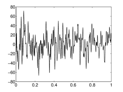
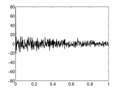
The impulsive noise is simulated by randomly taking 200 pulses in (27). The system’s motion is simulated as a linear combination of 100 functions (25) the frequencies of which are taking, randomly, from the set $[1,405]$. The data are assumed to be known in single precision. The simulation was run 50 times and in all the cases the cancellation of the impulsive noise was successful. The left graph of Fig. 1 plots one of the realizations of the experiment (motion of the system plus impulsive noise vs time). The graph on the right depicts the result obtained by applying the proposed technique to the signal on the left (it coincides with the line representing the true signal). On the contrary, although the spaces (27) and $\text{span}\{x_{n}(t),\,t\in[0,1]\}_{n=1}^{405}$ are ‘theoretically’ complementary, since the construction of the corresponding oblique projector is very ill posed, the projection fails to correctly separate the signals.

Figure 1: The left graph depicts the register of the motion of a system consisting of 100 damped harmonic oscillators, whose frequencies are integer numbers randomly taken from the interval $[1,405]$, corrupted by 200 pulses randomly taken from the subspace ${\cal{W}^{\bot}}$ given in (27). The graph on the right depicts the result of filtering the signal of the previous graph by the strategy described in Section 5. The result coincides with the true motion of the simulated system.

6.2 Application to the separation of a spectrum from blackbody radiation background

We consider an hypothetical situation where the background is assumed to be produced by a linear combination of up to five blackbodies (e.g. stars) at temperatures of $T_{1}=3000$K, $T_{2}=3500$K , $T_{3}=4000$K, $T_{4}=4500$K , and $T_{5}=5000$K. Hence, in this case the subspace ${\cal{W}^{\bot}}$ is defined as ${\cal{W}^{\bot}}=\text{span}\{y_{i}\}_{i=1}^{5}$, where $y_{i}$ are functions of the wavelength $\lambda$ as given by

$$y_{i}(\lambda)=\frac{C_{1}}{\lambda^{5}(e^{\frac{C_{2}}{\lambda T_{i}}}-1)},\quad C_{1}=3.7419\times 10^{-6}{\rm{erg\,cm^{2}\,s^{-1}}},C_{2}=1.4288{\rm{cm\,K}}.$$

Any linear combination of these functions is an acceptable background. In our numerical experiment the background, $y(\lambda)$, is generated as $y(\lambda)=\sum_{i=1}^{5}y_{i}(\lambda)$.

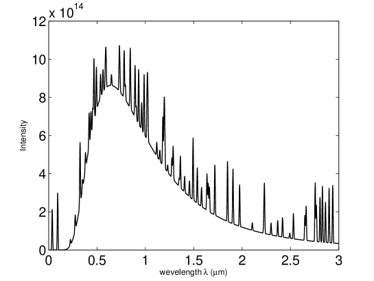
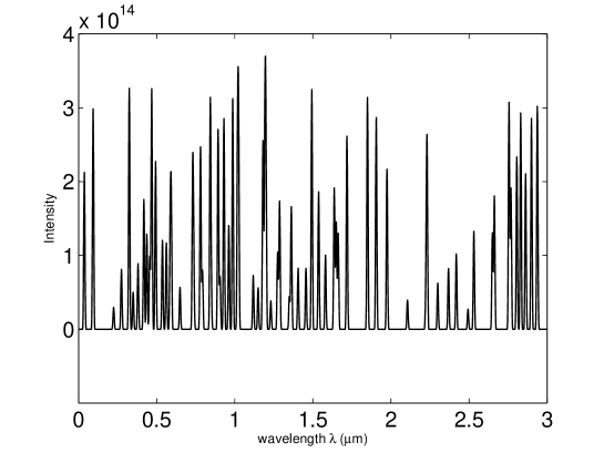
We simulate a spectrum, on a region of $\lambda$ ranging from zero to $3\mu\rm{m}$, by considering that it belongs to the cardinal cubic spline space on the interval $[0,3\mu\rm{m}]$ with separation $b=2^{-4}\mu\rm{m}$ between consecutive knots. Such a space can be spanned by a B-spline basis arising by translating a prototype B-spline [30, 31]. Different spectra are simulated by randomly drawing $K=70$ functions $\{v_{\ell_{i}}\}_{i=1}^{70}$, from the basis consisting of $483$ functions, to generate the decomposition $\sum_{i=1}^{70}c_{i}v_{\ell_{i}}$, with random coefficients $c_{i}\in[0,1],\,i=1\ldots,70$. A particular realization is depicted in the bottom graph of Fig. 2. The simulated available signal is obtained by adding the background $y(\lambda)$ given above to the spectrum, and perturbing each data point with a normal distributed error of variance corresponding to a percentage of each data value. Let us remark that, although the background is not ‘exactly’ in the cardinal spline space of the spectrum, it has a very good representation in such a space. Hence, the calculation of an oblique projector onto the given spline space and along the space of the background is expected to be very badly conditioned. Indeed, for very small errors (variance of $10^{-6}\%$ of each data value) the separation of the spectrum from the background is not possible by an oblique projection onto the whole spline space. However, in a simulation of 100 different spectra, each of which consisting of 70 randomly taken B-spline functions, the separation was successful in all the cases by applying the proposed approach. Thus, a more realistic situation was simulated by increasing the variance of the error up to $1\%$ of each data value. Also in this case the spectrum recovery was a complete success. In order to make evident the errors’ effect, the variance was increased up to $5\%$ of each data value. One of the simulations is plotted in the top graph of Fig. 3. The middle graph of the same figure shows both, the theoretical ‘hidden’ spectrum and the one recovered by the proposed approach. This graph is meant to illustrate a ‘typical result’, as in a run of the 100 simulations described above the reconstruction of the corresponding spectra was of similar quality. The visualization of the approximation quality is made clearer in the bottom graph of Fig. 3, where a portion of the previous graph (corresponding to the interval $[0.5,1]$) is plotted. Here we can see that, as expected, the approximation (broken line) fails to reproduce the peaks of low intensity (the one at $0.65\mu\rm{m}$). This is of course understandable by comparing the intensity of the spectrum with the intensity of the data on the $[0.5,1]$ interval. In this region, a variance of $5\%$ of intensity of each data point entails an uncertainty of more than one unit in the corresponding scale of intensity. Thus, one cannot expect to correctly spot peaks of intensity of the same order as the errors. On the other hand, some spurious peaks which are not in the true spectrum may also appear (note the small peak of negative intensity). However, on the whole we can confidently assert that the recovery of the simulated spectra is satisfactory even for significant error level. It is pertinent to point out that if one wished to avoid negative intensities one could penalize the selection of measurements leading to such negative values. In our framework this is implementable in a straightforward manner. For instance, in the forward selection procedure, at iteration $k+1$ we select the index $\ell_{k+1}$ satisfying (21) and it follows from (11) and (15) that the spectral intensity vector at this step is given as

$$|f_{{\cal{V}}_{k+1}}\rangle=|f_{{\cal{V}}_{k}}\rangle-\hat{E}_{{\cal{V}}_{k}}|v_{\ell_{k+1}}\rangle\frac{\langle\gamma_{k+1}|f\rangle}{|||\gamma_{k+1}\rangle||^{2}}+|v_{\ell_{k+1}}\rangle\frac{\langle\gamma_{k+1}|f\rangle}{|||\gamma_{k+1}\rangle||^{2}},$$ (28)

where $|f_{{\cal{V}}_{k}}\rangle$ is the spectral intensity obtained in the previous iteration, $\hat{E}_{{\cal{V}}_{k}}$ the oblique projector onto the previously selected subspace, $|f\rangle$ the observed data vector and $|\gamma_{k+1}\rangle$ (constructed as in (13)) is to be determined in the selection process of the index $\ell_{k+1}$ according to the prescription of Proposition 1. Thus, restrictions on $|f_{{\cal{V}}_{k+1}}\rangle$ can be incorporated by disregarding the selected indices yielding unacceptable values of $|f_{{\cal{V}}_{k+1}}\rangle$. In the example we are discussing here, one can avoid negative values of intensity by disregarding those indices which satisfying (21) do not fulfill the condition $\langle\lambda|f_{{\cal{V}}_{k+1}}\rangle=f_{{\cal{V}}_{k+1}}(\lambda)\geq 0$ for the values of $\lambda$ being considered. With the incorporation of this constrain the small negative pick in the middle graph of Fig. 3 disappears and the whole approximation improves. However, in some other realizations of the experiment when introducing the possibility constrains some small spurious picks of positive intensity appear, yielding on the whole an approximation of quality comparable with the unconstrained one. The spurious small peaks (or the absence or small peaks present in the true spectrum) are consequence of the considerable uncertainty in the data. The fidelity of the approximation with the true spectrum (in all the realizations of the experiment) is improved by reducing the error of the data.

7 Conclusion

The construction of measurement vectors specially designed for separating signal components produced by phenomena of different nature was discussed. Assuming that the subspaces hosting the signal components are given, the required measurement vectors should yield an oblique projection along one of the subspaces and onto the other. Considerations were restricted to those cases for which such subspaces are theoretically complementary, yet very close to each other, so that the construction of the measurement vectors for the whole space renders an ill posed problem. A recursive strategy for finding the right subspace to achieve the desired signal separation was then discussed. By recourse to numerical simulations it was illustrated that, provided that the signal is sparse in a spanning set of the signal subspace, the required signal splitting may be achieved by means of adaptive greedy techniques capable of searching for the required subspace while maintaining stability in the calculations. When tested in situations involving significant level of errors the proposed technique produced satisfactory results. Therefore, we are led to conclude that the framework for measurement design advanced here should be of assistance to a variety of applications where the discrimination of phenomena of different nature is required.

Acknowledgements

Support from EPSRC (EP$/$D062632$/$1) is acknowledged.

Figures

Figure 2: The top graph depicts theoretical data produced by the superposition of the spectrum shown in the bottom graph and black body radiation background.

Figure Caption

Figure 3. The top graph has the same description as the top graph of Fig. 2, but the data are perturbed with zero mean normal distributed errors of variance corresponding to $5\%$ of each data value. The continuous line in the middle graph represents the theoretical spectrum and the dotted line the spectrum obtained by the proposed approach from the data of the top graph. The bottom graph magnifies the region [0.5 1] in the previous graph.

References

- [1] R. Behrens, L. Scharf, Signal processing applications of oblique projection operators, IEEE Transactions on Signal Processing 42 (1994) 1413–1424.
- [2] L. Rebollo-Neira, Constructive updating/downdating of oblique projectors: a generalization of the Gram–Schmidt process, Journal of Physics A: Mathematical and Theoritcal 40 (2007) 6381–6394.
- [3] K. Jones, On a conjecture of huber concerning the convergence of projection pursuit regression, Ann. Stat. 15 (2) (1987) 880–882.
- [4] S. Mallat, Z. Zhang, Matching pursuits with time-frequency dictionaries, IEEE Transactions on Signal Processing 41 (1993) 3397–3415.
- [5] G. Davis, S. Mallat, M. Avellaneda, Adaptive greedy approximations, Constructive Approximation 13 (1) (1997) 57–98.
- [6] L. Rebollo-Neira, D. Lowe, Optimized orthogonal matching pursuit approach, IEEE Signal Processing Letters 9 (2002) 137–140.
- [7] M. Andrle, L. Rebollo-Neira, E. Sagianos, Backward-optimized orthogonal matching pursuit approach, IEEE Signal Proc. Let. 11 (2004) 705–708.
- [8] J. Tropp, Greed is good: algorithmic results for sparse approximation, IEEE Transactions on Information Theory 50 (10) (2004) 2231–2242.
- [9] M. Andrle, L. Rebollo-Neira, A swapping-based refinement of orthogonal matching pursuit strategies, Signal Processing 86 (2006) 480–495.
- [10] Y. Wu, V. S. Batista, Matching-pursuit for simulations of quantum processes, Journal of Chemical Physics 118 (2003) –.
- [11] Y. Wu, V. S. Batista, Quantum tunneling dynamics in multidimensional systems, Journal of Chemical Physics 121 (2004) –.
- [12] Q. Jie, Approximating the ground state of fermion systems by multiple determinant states: Matching pursuit approach, Phys. Rev. E 77 (2008) 026705.
- [13] L. Rebollo-Neira, Oblique matching pursuit, IEEE Signal Processing Letters 14 (10) (2007) 703–706.
- [14] S. Mallat, A Wavelet Tour of Signal Processing, 2nd Edition, Academic Press, London, 1999.
- [15] M. Reed, B. Simon, Functional Analysis, Academic Press, London, 1980.
- [16] D. Donoho, Compressed sensing, IEEE Trans. on Information Theory 52 (2006) 1289–1306.
- [17] E. Candès, J. Romberg, Quantitative robust uncertainty principles and optimally sparse decompositions, Foundations of Comput. Math. 6 (2006) 227–254.
- [18] E. Candès, T. Tao, Near optimal signal recovery from random projections: Universal encoding strategies?, IEEE Trans. on Information Theory 52 (2006) 5406–5425.
- [19] R. Baraniuk, A lecture on compressive sensing, IEEE Signal Processing Magazine.
- [20] Compressive sensing resources, http://www.dsp.ece.rice.edu/cs/See references listed there.
- [21] A. Galantai, Projectors and Projection Methods, Kluwer Academic Publishers, London, 2004.
- [22] Y. Eldar, Sampling with arbitrary sampling and reconstruction spaces and oblique dual frame vectors, Journal of Fourier Analysis and Applications 9 (2003) 77–96.
- [23] L. Rebollo-Neira, A. Plastino, Nonextensive maximum-entropy-based formalism for data subset selection, Phys. Rev. E 65 (1) (2002) –.
- [24] L. Rebollo-Neira, A. Plastino, A recursive approach for constructing the maxent distribution from redundant data, Phys. Rev. E 66 (3) (2002) –.
- [25] L. Rebollo-Neira, A. Plastino, Constructive approximations of the maximum entropy distribution from redundant and noisy data, Phys. Rev. E 70 (1) (2004) –.
- [26] M. Unser, A. Aldroubi, A general sampling theory for nonideal acquisition devices, IEEE Trans. Signal Processing 42 (1994) 2915–2925.
- [27] L. Rebollo-Neira, Backward adaptive biorthogonalization, International Journal of Mathematics and Mathematical Science 2004 (35) (2004) 1843–1853.
- [28] M. Andrle, L. Rebollo-Neira, Biorthogonal techniques for optimal signal representation, http://www.ncrg.aston.ac.uk/Projects/BiOrthog.
- [29] M. Andrle, L. Rebollo-Neira, Improvement of orthogonal matching pursuit strategies by backward and forward movements, in: Proc. of the 31st International Conference on Acoustics, Speech, and Signal Processing, Vol. 3, 2006, pp. III–III.
- [30] L. Schumaker, Spline Functions: Basic Theory, Wiley, New York, 1981.
- [31] M. Andrle, L. Rebollo-Neira, Cardinal B-spline dictionaries on a compact interval, Applied and Computational Harmonic Analysis 18 (2005) 336–346.