Controlling the Sign of Magnetoconductance in Andreev Quantum Dots

Abstract

We construct a theory of coherent transport through a ballistic quantum dot coupled to a superconductor. We show that the leading-order quantum correction to the two-terminal conductance of these Andreev quantum dots may change sign depending on (i) the number of channels carried by the normal leads or (ii) the magnetic flux threading the dot. In contrast, spin-orbit interaction may affect the magnitude of the correction, but not always its sign. Experimental signatures of the effect include a non-monotonic magnetoconductance curve and a transition from an insulator-like to a metal-like temperature dependence of the conductance. Our results are applicable to ballistic or disordered dots.

Introduction. Low temperature experiments on diffusive metals coupled to superconductors have reported large interference effects analogous to coherent backscattering, weak-localization and Aharonov-Bohm oscillations Vanson87 ; Pet93 ; Cou96 ; Har97 ; Eom98+Jia05 ; Par03 ; Bau08 , one to two orders of magnitude above the universal amplitude ${\cal O}(e^{2}/h)$ they have in purely metallic mesoscopic conductors Akkermans . In some cases, a weak localization-like behavior, in the form of positive magnetoconductance near zero field is observed Par03 ; Bau08 , but often one sees negative magnetoconductance Pet93 ; Cou96 ; Har97 ; Eom98+Jia05 . Theoretical works predict that Andreev reflection from the superconductor induces this large quantum correction to transport Spi82 ; Bee95 . The general expectation is that this correction is similar to a magnified weak-localization correction, in that its sign is determined by the presence or absence of spin-orbit interaction (SOI) Akkermans ; Hik80 . In this paper we revisit this issue, and find that this interference correction has very different properties from weak-localization. In particular, we show that both the specific lead-geometry and an applied magnetic flux can reverse its sign, while SOI need not.

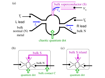
Figure 1: (a) A two-dimensional Andreev quantum dot in a three-terminal geometry, with two normal (N) and one superconducting (S) lead. (b,c) The two possible two-terminal set-ups obtained from such a dot. Either (b) the S lead is contacted to one of the N leads, or (c) the S lead is floating.

Andreev reflection And64 is the dominant low energy process at the interface between a metal and a superconductor. It involves an electron (hole) being retroreflected as a hole (electron) and retracing the path previously followed by the electron (hole). In this article, we extend the trajectory-based semiclassical theory to include Andreev reflection, analyze the conductance of a two-dimensional ballistic quantum dot coupled to one superconducting lead and two normal leads, as in Fig. 1. We dub this system an Andreev quantum dot. We arrive at the surprising conclusion that the interference effects can be reversed from localizing to antilocalizing by changing the widths of the normal leads, or by threading a fraction of a magnetic flux quantum through the dot. In contrast SOI need not cause such a reversal. This is very different from weak-localization in purely metallic conductors, whose sign is solely determined by the presence or absence of SOI Akkermans ; Hik80 ; caveat . We predict two clear experimental signatures of these interference effects in the form of non-monotonic magnetoconductance curves (see Fig. 3) and a transition from an insulator-like to a metal-like temperature-dependence of the conductance as one changes the magnetic field or the ratio of the lead widths. This transition occurs because thermal averaging destroys quantum interferences, thus depending on the sign of the effect, the conductance increases or decreases by many times $e^{2}/h$ as the temperature increases.

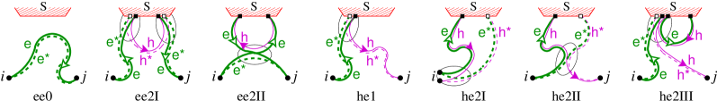
Figure 2: Contributions to $\langle T_{ij}^{\rm ee}\rangle$ (first three) and $\langle T_{ij}^{\rm he}\rangle$ (last four) considered in this letter. Thick green (thin violet) paths indicate electrons (holes), dashed lines indicate complex-conjugated amplitudes. Normal leads are labelled $i,j$ while the S lead is superconducting. The contributions are classified by the number of uncorrelated Andreev reflections (ee0 has none, ee2I and ee2II both have two). The full (open) squares on the S lead indicate a factor of $\eta$ ($\eta^{*}$) and the ellipses mark encounters.

Semiclassical transport with superconductivity. According to the scattering approach to transport, the current in normal lead $i$ is given by Lam93

$$I_{i} = {2e\over h}\int_{0}^{\infty}{\rm d}\varepsilon\sum_{j}\left[2N_{i}\delta_{ij}-T_{ij}^{\rm ee}+T_{ij}^{\rm he}-T_{ij}^{\rm hh}+T_{ij}^{\rm eh}\right]$$ (1)

$$\hskip 62.59596pt\times(-\partial f/\partial\varepsilon)(\mu_{j}-\mu_{\rm S})\,,$$

where $\mu_{j}$ is the chemical potential of normal (N) lead $j$ and $\mu_{\rm S}$ of all the superconducting (S) leads. The Fermi-Dirac distribution, $f(\varepsilon)$, has $\varepsilon$ measured from $\mu_{\rm S}$. Here we use trajectory-based semiclassics to find the scattering probability $T_{ij}^{\alpha\beta}$ to go from quasiparticle $\beta={\rm e,h}$ (electron, hole) in lead $j$ to quasiparticle $\alpha$ in lead $i$. Extending trajectory-based semiclassics Ric02 ; Whi06 ; Essen-papers ; Bro06 ; Ber08 to include Andreev reflection, one has Goo08

$$T_{ij}^{\alpha\beta} = \frac{1}{2\pi\hbar}\int_{j}{\rm d}y_{0}\int_{i}{\rm d}y\sum_{\gamma 1,\gamma 2}A_{\gamma 1}A_{\gamma 2}^{*}\exp[i\delta S/\hbar]\,.\qquad$$ (2)

This expression sums over all classical trajectories $\gamma 1$ and $\gamma 2$ entering the cavity at $y_{0}$ on a cross-section of lead $j$ and exiting at $y$ on a cross-section of lead $i$, while converting a $\beta$ quasiparticle into an $\alpha$ quasiparticle. The phase $\delta S=S_{\gamma 1}-S_{\gamma 2}$ gives the difference in action phase accumulated along $\gamma 1$ and $\gamma 2$, and $A_{\gamma}$ gives the stability of the trajectory $\gamma$. In contrast to Ref. Goo08 , we consider the physically more prevalent situation of an Ehrenfest time negligible against the dwell time $\tau_{\rm D}$ inside the dot. In that case, even with perfect Andreev reflection, quantum uncertainties combined with the chaotic dynamics make the retroreflected quasiparticle diverge from the incoming quasiparticle path well before it leaves the dot Lar68 . Therefore classical paths undergoing Andreev reflections consist of electron and hole segments that do not necessarily retrace each other all the way. For transmission probabilities $\langle T_{ij}^{\alpha\beta}\rangle$ averaged over energy or dot shape, we must pair the paths $\gamma 1$ and $\gamma 2$ in Eq. (2) in ways that render their action phase difference stationary. To do this we either pair a path with a complex conjugate path, e-e^∗ or h-h^∗, or we pair an electron path with a hole path, e-h or e^∗-h^∗. Path-pairs can meet and swap pairings at encounters, as shown in Fig. 2. Following Ref. Whi06 we distinguish between encounters that lie entirely inside the dot and those that touch a lead.

Feynman rules. Contributions relevant to current noise in purely metallic samples Whi06 ; Essen-papers ; Bro06 ; Ber08 , become relevant for the calculation of the current itself in the presence of S leads when they can be made from only two classical trajectories with some segments as electron and others as holes. From Refs. Whi06 ; Bro06 ; Ber08 and the above considerations, we derive the following Feynman rules for calculating transmission through an Andreev quantum dot. The dot is connected to normal and superconducting leads, each carrying $N_{i}\gg 1$ and $N_{{\rm S}j}\gg 1$ transport channels respectively, and we write $N_{\rm T}=\sum_{i}N_{i}+\sum_{j}N_{{\rm S}j}$ For a perpendicular magnetic field, $b=B/B_{\rm c}$, measured in units of the field $B_{\rm c}\simeq(h/eA)(\tau_{0}/\tau_{\rm D})^{1/2}$ that breaks time-reversal (TR) symmetry in a quantum dot of area $A$ with time of flight $\tau_{0}$, the Feynman rules read:

(i) An e-e^∗ or h-h^∗ path-pair gives a factor of $[N_{\rm T}(1+\chi b^{2})]^{-1}$, with $\chi=1$ for time-reversed paths and $\chi=0$ otherwise.
(ii) An e-h or e^∗-h^∗ path-pair gives $N_{\rm T}^{-1}\times(1\pm{\rm i}2\varepsilon\tau_{\rm D}+\chi b^{2})^{-1}$, with upper (lower) sign for e-h (e^∗-h^∗).
(iii) An encounter inside the dot and connecting e,e^∗, h and h^∗ paths (as in he2II) gives a factor $-N_{\rm T}$.
(iv) An encounter inside the dot and connecting e, e, e^∗ and h paths (as in ee2II) gives a factor of $-N_{\rm T}(1+{\rm i}2\varepsilon\tau_{\rm D}+b^{2})$; this factor is complex conjugated (c.c.) for an encounter connecting e, e^∗, e^∗ and h^∗ paths.
(v) An encounter touching a N lead $i$ (S lead $j$) gives a factor of $N_{i}$ ($N_{{\rm S}j}$).
(vi) A path-pair that ends at a N lead $i$ (S lead $j$), while not in an encounter, gives a factor of $N_{i}$ ($N_{{\rm S}j}$).
(vii) Andreev reflections at S leads involving e$\to$h give a factor of $\eta\,{\rm e}^{-\rm i\Phi_{{\rm S}j}}$ while those involving h$\to$e give a factor of $\eta\,{\rm e}^{\rm i\Phi_{{\rm S}j}}$ (e${}^{*}\to$h^∗ and h${}^{*}\to$e^∗ give the c.c. of these factors), where $\Phi_{{\rm S}j}$ is the S phase on lead $j$, and $\eta=\exp[-{\rm iarcos}\,(\varepsilon/\Delta)]$ is the Andreev reflection phase.

We note that these rules equally follow from random-matrix theory Essen-papers .

In our analysis of the consequences of these rules, we consider temperatures well below the superconducting gap $\Delta$ where $\eta=-{\rm i}$, and consider a single S lead (setting $\Phi_{\rm S}=0$ without loss of generality). The rules indicate that a path-pair going from encounter to encounter reduces the contribution by a factor of ${\cal O}[N_{\rm T}]$. Thus to leading order in $N_{\rm T}$, we can neglect such (weak localization) contributions. This does not restrict the number of encounters, because the price to add an encounter whose additional legs go to S leads is ${\cal O}[(N_{\rm S}/N_{\rm T})^{2}]$. We therefore take $N_{\rm S}/N_{\rm T}\ll 1$, and expand in the number of uncorrelated Andreev reflections.

Restricting ourselves to ${\cal O}[(N_{\rm S}/N_{\rm T})^{2}]$, we need to consider the contributions shown in Fig. 2 involving no more than two uncorrelated Andreev reflections. The contributions to $\langle T^{\rm ee}_{ij}\rangle$ are

$$\langle T^{\rm ee0}_{ij}\rangle = N_{i}N_{j}/N_{\rm T},$$ (3a)

$$\langle T^{\rm ee2I}_{ij}\rangle = N_{i}N_{j}N_{\rm S}^{2}/N_{\rm T}^{3},$$ (3b)

$$\langle T^{\rm ee2II}_{ij}\rangle = {2N_{i}N_{j}N_{\rm S}^{2}\over N_{\rm T}^{3}}\,{\rm Re}\left[(1+b^{2}+{\rm i}2\varepsilon\tau_{\rm D}^{2})^{-1}\right].$$ (3c)

The contributions to $\langle T^{\rm he}_{ij}\rangle$ are

$$\langle T^{\rm he1}_{ij}\rangle = N_{i}N_{j}N_{\rm S}/N_{\rm T}^{2},$$ (4a)

$$\langle T^{\rm he2I}_{ij}\rangle = \delta_{ij}\,N_{i}N_{\rm S}^{2}/\left[N_{\rm T}^{2}\big{(}(1+b^{2})^{2}+4\varepsilon^{2}\tau^{2}_{\rm D}\big{)}\right],$$ (4b)

$$\langle T^{\rm he2II}_{ij}\rangle = -N_{i}N_{j}N_{\rm S}^{2}/\left[N_{\rm T}^{3}\big{(}(1+b^{2})^{2}+4\varepsilon^{2}\tau^{2}_{\rm D}\big{)}\right],\qquad\$$ (4c)

$$\langle T^{\rm he2III}_{ij}\rangle = -\langle T^{\rm ee2II}_{ij}\rangle.$$ (4d)

Semiclassics gives $\langle T_{\rm ij}^{\rm hh}\rangle=\langle T_{\rm ij}^{\rm ee}\rangle$ and $\langle T_{\rm ij}^{\rm eh}\rangle=\langle T_{\rm ij}^{\rm he}\rangle$. These contributions preserve unitarity up to and including ${\cal O}[(N_{\rm S}/\sum_{i}N_{i})^{2}]$.

Set-up with an S lead. We first consider the situation where the S lead’s potential is fixed externally. This may be the three-terminal device of Fig. 1a with both the R and S leads grounded, while the L lead is biased at electrochemical potential $\mu_{\rm L}=eV$. Alternatively this may be the two-terminal device in Fig. 1b with the S and R leads join at a bulk contact (with contact conductance vastly greater than the dot), a macroscopic distance away from the dot. In either case, the L lead current is $I_{\rm L}=(2e^{2}/h)\left[g_{\rm cl}+\delta g_{\rm qm}(T,b)\right]V$, where we define a dimensionless classical conductance $g_{\rm cl}=N_{\rm L}(N_{\rm R}+2N_{\rm S})/(N_{\rm L}+N_{\rm R}+2N_{\rm S})$ footnote:drude . For $N_{S}\ll N$ the quantum interference correction is

$$\delta g_{\rm qm}=\frac{N_{\rm L}[N_{\rm R}-4N_{\rm L}(1+b^{2})]N_{\rm S}^{2}}{(N_{\rm L}+N_{\rm R})^{3}}f(T,b)+\delta g_{\rm wl}.$$ (5)

In the regime of experimental interest the weak-localization correction in the absence of the S lead $\delta g_{\rm wl}\simeq-N_{\rm L}N_{\rm R}/[(N_{\rm L}+N_{\rm R})^{2}(1+b^{2})]$ is small enough to neglect (as in Fig. 3). The $\varepsilon$-integral in Eq. (1) with $\langle T_{ij}^{\alpha\beta}\rangle$ in Eqs. (3,4) leads to $f(T,b)=\alpha\,\zeta(2,1/2+(1+b^{2})\alpha)$, with $\alpha=E_{\rm T}/4\pi k_{\rm B}T$ for a Thouless energy $E_{\rm Th}=\hbar/\tau_{\rm D}$, and the generalized $\zeta$-function $\zeta(2,x)=\int_{0}^{\infty}t\exp[-xt]/(1-\exp[-t]){\rm d}t$. This gives the two asymptotics $f(T\rightarrow\infty,b)\rightarrow\pi E_{\rm T}/[8k_{\rm B}T(1+b^{2})]$ and $f(T\rightarrow 0,b)\rightarrow 1/(1+b^{2})^{2}$.

At zero temperature, we find three regimes for $\delta g_{\rm qm}$:

(a) For $N_{\rm R}<2N_{\rm L}$, $\delta g_{\rm qm}<0$ for all values of $b$, and gives a monotonic magnetoconductance curve.

(b) For $2N_{\rm L}<N_{\rm R}<4N_{\rm L}$, $\delta g_{\rm qm}<0$ for all $b$, but gives a non-monotonic magnetoconductance, with a minimum at $b^{2}=(N_{\rm R}-2N_{\rm L})/(2N_{\rm L})$.

(c) For $N_{\rm R}>4N_{\rm L}$, $\delta g_{\rm qm}>0$ at small $b$, but becomes negative for $b^{2}>(N_{\rm R}-4N_{\rm L})/(4N_{\rm L})$, and then goes to zero for large $b$. As in (b), the curve is non-monotonic with minima at $b^{2}=(N_{\rm R}-2N_{\rm L})/(2N_{\rm L})$.

These different regimes persist at finite temperature as is illustrated in Fig. 3, however, the boundary between (a) and (b), as well as the positions of the minima of the magnetoconductance curves are $T$-dependent. The conductance exhibits a metal-like (insulating-like) behavior in the form of a decrease (increase) of the conductance with $T$, depending on the sign of $(N_{\rm R}-4(1+b)^{2}N_{\rm L})$. This sign can easily be changed, whenever one has control over the lead widths or the magnetic flux. Remarkably, a monotonic magnetoconductance may become non-monotonic upon increase of the temperature (dashed red curves in Fig. 3).

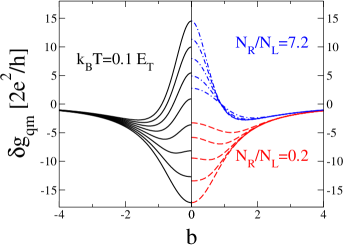
Figure 3: Magnetoconductance curves for the set-up of Fig. 1b. Left panel: $k_{\rm B}T=0.1E_{\rm T}$, and $N_{\rm R}/N_{\rm L}=n+0.2$, $n=0,1,2,...7$ (from bottom to top). Right panel: $N_{\rm R}/N_{\rm L}=0.2$ (dashed red) and $7.2$ (dot-dashed blue), for $k_{\rm B}T/E_{\rm T}=0.1$, 1, 2, 4 and 8 (dashed: from bottom to top; dot-dashed: from top to bottom). For both panels, the vertical axis gives $\delta g_{\rm qm}$ in units of the conductance quantum $2e^{2}/h$ with channel numbers chosen such that $N_{\rm S}^{2}N_{\rm L}^{2}/(N_{\rm L}+N_{\rm R})^{3}=5$ in all instances. Note the crossover from monotonic to non-monotonic behavior of the magnetoconductance as $T$ increases, for $N_{\rm R}/N_{\rm L}=0.2$ (dashed red curves).

Set-up with an S island. In the second of the two possible two-terminal set-ups, Fig. 1c), the quantum dot is connected to a superconducting island, whose chemical potential is floating, and adapts itself to a value guaranteeing current conservation, $I_{\rm L}=-I_{\rm R}$. Using the expression in Ref. Lam93 for the two-terminal conductance in terms of the transmission probabilities, $T^{\alpha\beta}_{ij}$, we obtain $g=g^{\rm isl}_{\rm cl}+\delta g^{\rm isl}_{\rm qm}(T,b)$ where $g^{\rm isl}_{\rm cl}=N_{\rm L}N_{\rm R}/(N_{\rm L}+N_{\rm R})$ and $\delta g^{\rm isl}_{\rm qm}=N_{\rm L}N_{\rm R}N_{\rm S}^{2}(N_{\rm L}+N_{\rm R})^{-3}\,f(T,b)$. This reproduces the random matrix theory result Bee95 to leading order in $[N_{\rm S}/(N_{\rm L}+N_{\rm R})]^{2}$. This quantum correction always increase the conductance (antilocalization) by a parametrically large amount (many $e^{2}/h$), with a monotonic magnetoconductance curve.

Mesoscopic conductance fluctuations and current noise. Ref. Bro96 used random matrix theory to show that conductance fluctuations remain ${\cal O}(e^{2}/h)$ in the presence of superconductivity. Our Feynman rules reproduce this result. Contributions to ${\rm var}[g]$ are the product of any two contributions in Fig. 2 connected by encounters. Since path-pairs are not swapped at entrance and exit, the connection must involve at least two additional encounters with four additional path-pairs, and the resulting contribution behaves as $N_{\rm T}^{-2}$ times the average conductance squared. This is at most ${\cal O}[N_{\rm T}^{0}]$, thus the quantum corrections to the average conductance are parametrically larger than the conductance fluctuations, and are therefore easily observable.

The S contact also leads to e-h contributions to the current-noise Ana96 . The Feynman rules show that they are ${\cal O}[N_{\rm T}(N_{\rm S}/N_{\rm T})^{n}]$ for $n\geq 1$ and are thus smaller than the ${\cal O}[N_{\rm T}]$ e-e contributions which give the noise in the absence of an S lead. Therefore, to leading order in $N_{\rm S}/N_{\rm T}$, the parametric magnitude of the zero-frequency current-noise is unaltered by the presence of the S lead.

Effect of SOI. Spin-orbit interaction (SOI) can be treated as rotating the spin along otherwise unchanged classical trajectories, multiplying Eq. (2) by ${\rm Tr}[d_{\gamma 1}d_{\gamma 2}^{\dagger}]$, where $d_{\gamma i}$ is the SU(2)-phase of path $\gamma i$ Mat92 . For ee0, ee2I and he1, this gives a factor of two for spin-degeneracy, because $d_{\gamma 1}=d_{\gamma 2}$. However for ee2II and he2III it gives ${\rm Tr}[d_{1}^{2}]$, and for he2I and he2II it gives ${\rm Tr}[d_{1}^{2}d_{2}^{2}]$, where $d_{1},d_{2}$ are statistically independent random SU(2) phases. When the SOI time is shorter than $\tau_{\rm D}$, one averages uniformly over the SU(2) phases Zai05 , which multiplies ee2II and he2III by $-1/2$, and he2I and he2II by $1/4$. Taking $T=0$ and neglecting $\delta g_{\rm wl}$ for simplicity, we find that

$$\delta g_{\rm qm} = {N_{\rm L}\,[(1-2/\beta)^{2}N_{\rm R}+4(1-2/\beta)N_{\rm L}]\,N_{\rm S}^{2}\over(N_{\rm L}+N_{\rm R})^{3}},\qquad$$ (6a)

$$\delta g^{\rm isl}_{\rm qm} = {(1-2/\beta)^{2}N_{\rm L}N_{\rm R}N_{\rm S}^{2}/(N_{\rm L}+N_{\rm R})^{3}},$$ (6b)

for the three standard symmetry classes, $\beta=1$ (TR symmetry without SOI), 2 (no TR symmetry) and 4 (TR symmetry with SOI). Note the presence of the same symmetry prefactor $(1-2/\beta)$ as for weak localization without superconductivity. Thus with SOI ($\beta=4$), both $\delta g_{\rm qm}$ and $\delta g^{\rm isl}_{\rm qm}$ always enhance conductance. Therefore, SOI must be absent for a sign change of $\delta g_{\rm qm}$ with lead width. Turning on SOI (going from $\beta=1$ to $\beta=4$) never changes the sign of $\delta g^{\rm isl}_{\rm qm}$ but changes the sign of $\delta g_{\rm qm}$ for $N_{\rm R}<4N_{\rm L}$.

Concluding remarks. The derivation outlined here is for ballistic quantum dots, however the Feynman rules that we analyze apply to any system well-modelled by random matrix theory. Thus our results are equally applicable to disordered dots. We also expect qualitatively similar behaviors in diffusive metals coupled to superconductors at intermediate temperatures, $k_{\rm B}T\sim E_{\rm T}$. Work in this regime is in progress.

Upon completion of this work, we noted Ref. Regensburg-gang which uses a somewhat similar methodology as ours in closed Andreev billiards. RW thanks L. Saminadayar and C. Bäuerle for stimulating discussions, and access to their data Bau08 . PJ thanks the Physics Department of the Universities of Geneva and Basel as well as the Aspen Center for Physics for their hospitality at various stages of this project and acknowledges the support of the National Science Foundation under Grant No. DMR-0706319.

References

- (1) P.C. van Son, H. van Kempen, and P. Wyder, Phys. Rev. Lett. 59, 2226 (1987); J. Phys. F 18, 2211 (1988).
- (2) A. Parsons, I.A. Sosnin, and V.T. Petrashov, Phys. Rev. B 67, 140502(R) (2003).
- (3) V.T. Petrashov, V.N. Antonov, P. Delsing, and R. Claeson, Phys. Rev. Lett. 70, 347 (1993).
- (4) H. Courtois, Ph. Gandit, D. Mailly, and B. Pannetier, Phys. Rev. Lett. 76, 130 (1996).
- (5) S.G. den Hartog, B.J. van Wees, Yu.V. Nazarov, T.M. Klapwijk, and G. Borghs, Phys. Rev. Lett. 79, 3250 (1997).
- (6) J. Eom, C.-J. Chien, and V. Chandrasekhar, Phys. Rev. Lett. 81, 437 (1998); Z. Jiang and V. Chandrasekhar, Phys. Rev. B 72, 020502(R) (2005).
- (7) C. Bäuerle and L. Saminadayar, Private Comm. (2008).
- (8) E. Akkermans and G. Montambaux, Mesoscopic Physics of Electrons and Photons (Cambridge University, Cambridge, 2007).
- (9) B.Z. Spivak and D.E. Khmelnitskii, JETP Letters, 35, 412 (1982).
- (10) C.W.J. Beenakker, J.A. Melsen, and P.W. Brouwer, Phys. Rev. B 51, 13883 (1995).
- (11) S. Hikami, A.I. Larkin and Y. Nagaoka, Prog. Theor. Phys. 63, 707 (1980).
- (12) A.F. Andreev, Sov. Phys. JETP 19, 1228 (1964).
- (13) We exclude multiterminal measurements where the resistance is not necessarily an extremum at zero field. See: M. Büttiker, Phys. Rev. Lett. 57, 1761 (1986).
- (14) C. J. Lambert, J. Phys.: Cond. Mat. 5, 707 (1993).
- (15) K. Richter and M. Sieber, Phys. Rev. Lett. 89, 206801 (2002).
- (16) R.S. Whitney and Ph. Jacquod, Phys. Rev. Lett. 96, 206804 (2006).
- (17) P. Braun, S. Heusler, S. Müller, and F. Haake, J. Phys. A: Math. Gen. 39, L159 (2006).
- (18) P.W. Brouwer, and S. Rahav, Phys. Rev. B 74, 085313 (2006).
- (19) G. Berkolaiko, J.M. Harrison and M. Novaes, J. Phys. A 41, 365102 (2008).
- (20) M.C. Goorden, Ph. Jacquod, and J. Weiss, Phys. Rev. Lett. 100, 067001 (2008); Nanotechnology 19, 135401 (2008).
- (21) A.I. Larkin and Yu.N. Ovchinnikov, Zh. Eksp. Teor. Fiz. 55, 2262 (1968) [Sov. Phys. JETP 28, 1200 (1969)].
- (22) This expression for is correct to all orders in .
- (23) P.W. Brouwer and C.W.J. Beenakker, Phys. Rev. B 54, R12705 (1996).
- (24) M.P. Anantram and S. Datta, Phys. Rev. B 53, 16390 (1996).
- (25) H. Mathur and A.D. Stone, Phys. Rev. Lett. 68, 2964 (1992).
- (26) O. Zaitsev, D. Frustaglia, and K. Richter, Phys. Rev. B 72, 155325 (2005).
- (27) J. Kuipers, C. Petitjean, D. Waltner, and K. Richter, preprint – arXiv:0907.2660.