Investigation of quasi-periodic variations in hard X-rays of solar flares

Abstract

The aim of the present paper is to use quasi-periodic oscillations in hard X-rays (HXRs) of solar flares as a diagnostic tool for investigation of impulsive electron acceleration. We have selected a number of flares which showed quasi-periodic oscillations in hard X-rays and their loop-top sources could be easily recognized in HXR images. We have considered MHD standing waves to explain the observed HXR oscillations. We interpret these HXR oscillations as being due to oscillations of magnetic traps within cusp-like magnetic structures. This is confirmed by a good correlation between periods of the oscillations and the sizes of the loop-top sources. We argue that a model of oscillating magnetic traps is adequate to explain the observations. During the compressions of a trap particles are accelerated, but during its expansions plasma, coming from chromospheric evaporation, fills the trap, which explains the large number of electrons being accelerated during a sequence of strong impulses. The advantage of our model of oscillating magnetic traps is that it can explain both the impulses of electron acceleration and quasi-periodicity of their distribution in time.

1 Introduction

intr

Extreme ultraviolet (EUV) images from the TRACE satellite allowed to observe oscillations of coronal loops during solar flares (see asc04 and papers refereed therein). Typical periods of the oscillations were 200–300 s. The oscillations have been explained as standing MHD oscillations of whole coronal loops, i.e. with nodes located at the loop footpoints.

nak06 observed quasi-periodic oscillations (QPOs) with similar periods, $P=2-4$ min, in hard X-rays (HXRs) of a solar flare and similar periods, $P\approx 5$ min were observed in soft and hard X-rays of a solar flare by fou05. In both those papers the observed periodicities were also interpreted as being due to the oscillations of whole coronal loops.

On the other hand, in many flares QPOs with shorter periods, $P\simeq 10-60$ s, were observed in HXR emission (see lip78). In the present paper we would like to show how the investigation of these short-period oscillations can be used to investigate impulsive electron acceleration.

In Sect. obs observational data and their analysis are presented. Sect. sec:disc contains the discussion of our results and Sect. concl contains our conclusions.

In this paper we mostly investigate quasi-periodic HXR oscillations with periods $P\simeq 10$–60 s, but in Sect. llimb we present analysis of three limb flares with periods $P>120$ s.

2 Observations and their analysis

obs

We used HXR light-curves (recorded by Yohkoh and Compton Gamma Ray Observatory) and HXR images (recorded by Yohkoh). First, from the Yohkoh Hard X-ray Telescope Catalogue [Sato et al. (2006)] we selected flares which showed at least three HXR impulses and the time-intervals between the impulses were of similar duration (see Figs. limb1 and limb2). We have selected about 50 appropriate flares. Next, we investigated their HXR images and have taken for further analysis the flares for which the altitude and diameter of the HXR loop-top source could be reliably determined.

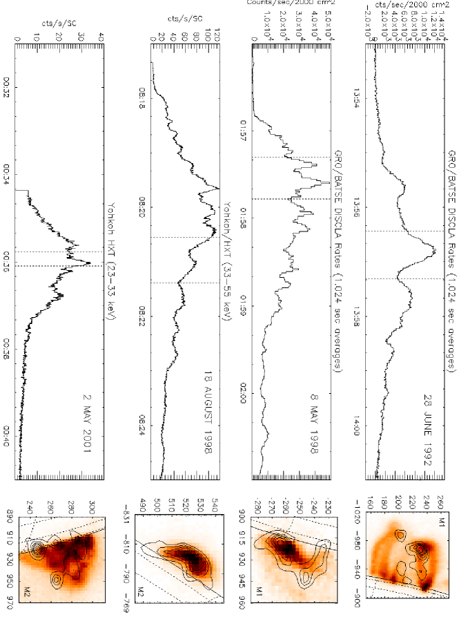
Figure 1.: Hard X-ray observations for four limb flares. Left: HXR light-curves (dashed vertical lines indicate accumulation times of the HXR images shown at the right). Right: Yohkoh HXR images of the flares (isolines 0.12, 0.24, 0.35, 0.47, 0.59, and 0.78 $I_{max}$) and SXR images (gray scale). Solid line shows solar limb and dashed lines are on the solar disc. The coordinates (x, y) are in arcsec, the zero-point located at the disc center.limb1

2.1 Limb flares with periods $P=10-60$ s

slimb

Table 1.: List of limb flares with periods $P$ = 10–60 s^atab1

Flare	Date; time [UT]	$P$	$h$	$v_{1}$	$B_{1}$	$d$	$v_{2}$	$B_{2}$
No.		[s]	[Mm]	[km s-1]	[G]	[Mm]	[km s-1]	[G]
1b	92/06/28; 13:54–14:00	56; 66	36	4040	184	14.0	785	36
2	98/05/08; 01:57–01:59	12; 18	18	9400	428	3.4	890	40
3	98/08/18; 08:18–08:23	21; 28	10	3000	136	8.5	1270	57
4	01/05/02; 00:35–00:37	24; (50)	24	6300	290	5.1	670	31

• Definition of parameters: $P$ are the time intervals between HXR peaks; $h$ is the altitude of a HXR loop-top source; $v_{1}$ is the velocity estimated according to Eq. (1); $B_{1}$ is the magnetic field strength calculated from Eq. (3); $d$ is the diameter of a HXR loop-top source; $v_{2}$ is the velocity estimated according to Eq. (4); $B_{2}$ is the magnetic field strength calculated from Eq. (5). Time interval is the interval in which the periods $P$ were determined.

• Structure and evolution of this flare was investigated by tom97.

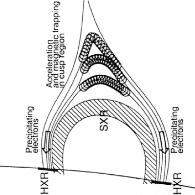
Figure 2.: A cusp-like (triangular) magnetic structure according to Aschwanden (2004). The tight spiral lines show motion of trapped electrons.cusp

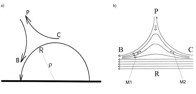
Figure 3.: a Schematic diagram showing a cusp-like magnetic configuration. Magnetic fields PB and CP reconnect at P. The thick horizontal line is the chromosphere. b Detailed picture of the BPC cusp-like magnetic structure.scheme

In this Section we investigate four limb flares. Their HXR light-curves and images are shown in Fig. limb1. We have measured the loop-top source diameter, $d$, on various images of the same HXR source and this way we have estimated its measuring (r. m. s.) error to be about ${\pm}1.5$ Mm. The loop-top source diameters and their altitudes, $h$, are given in Table tab1. In the Table two values of period $P$ are given for each flare. They were measured as the time-intervals between the strong HXR peaks. The shorter period, which corresponds to higher magnetic field compression, is taken in the estimates in Section 2 [Eqs. (1) and (4)]. By multiple measuring the same time interval, $P$, we have estimated the r. m. s. errors of the measurements to be about $\pm$2 s for sharp peaks and about $\pm$4 s for the peaks which are not sharp or fluctuating (see error bars in Fig. plot).

We have considered a hypothesis that the observed HXR oscillations are the result of fast kink-mode oscillations (see below about their excitation) and we have considered two kinds of magnetic structure where they occur:

1. a simple magnetic loop (no inflexion points on the magnetic lines),

2. a magnetic loop with a “cusp-like” structure at the top [Aschwanden’s asc04 model – see Fig. cusp].

In the first case the observed HXR QPOs are due to oscillations of whole flaring loops, i.e. the nodes of standing waves are situated at the loop footpoints. Assuming semi-circular shape of a loop, we can calculate the velocity of the wave:

$$v_{1}=\frac{2{\pi}{h}}{P}$$ (1)

The values of $P$, $h$ and $v_{1}$ are given in Table tab1.

For the MHD fast-mode oscillations it should be

$$v_{1}\approx v_{A}=B_{1}/\sqrt{4{\pi}{\rho}},$$ (2)

where $v_{A}$ is the Alfven speed and $B_{1}$ and $\rho$ are the mean magnetic field and mass density inside the oscillating loop. Hence

$$B_{1}\approx v_{1}\sqrt{4{\pi}{\rho}}.$$ (3)

k+l08 estimated the electron number density, $N$, for a number of HXR loop-top sources. Their values were concentrated between 5$\times$10⁹ cm^-3 and 5$\times$10¹⁰ cm^-3 with a peak around 1.0$\times$10¹⁰ cm^-3. Using this values of the electron density we have calculated values of the magnetic filed strength $B_{1}$ which are given in Table tab1.

mar06 investigated oscillations of flaring loops using Doppler-shifts in SXR spectra. The obtained distribution of periods showed maximum between 3 and 5 minutes. He interpreted those oscillations as being slow-mode or fast magnetosonic oscillations of whole flaring loops.

Our periods, $P=10-60$ s, are significantly shorter than those found by Mariska which suggests that the oscillations seen in HXRs occur in smaller magnetic structures (see also comment in Section sec:disc). On the other hand, the cusp-like magnetic structure is considered to be a “standard” magnetic structure in solar flares (see asc04). Therefore we have assumed that the oscillations seen in HXRs occur in such cusp-like structures.

Figure schemea shows a simple scheme of the cusp-like structure of Fig. cusp. Magnetic field lines steeply converge around B and C. Charged particles are efficiently reflected there (magnetic mirrors). Dynamics of the magnetic field inside the cusp volume BPC is explained in Fig. schemeb. Magnetic field PB and CP reconnect at P. This generates a sequence of magnetic traps which move downwards and collides with a stronger magnetic field R below. The collision causes compression, the magnetic and gas pressure increases inside the traps, so that the compression is stopped, the traps can expand and perform magnetosonic oscillations.

The excited fast magnetosonic waves propagate along the magnetic field lines, they meet regions of steep increase of Alfven speed near B and C, where they are efficiently reflected back into the trap. Hence, the magnetosonic waves will be efficiently trapped within the magnetic traps and we can describe them as standing fast magnetosonic (kink) oscillations trapped between B and C.

We can calculate the velocity of the waves

$$v_{2}=2s/P,$$ (4)

where $s$ is the distance between B and C taken along the magnetic field lines. Diameters, $d$, of the HXR loop-top sources have been used to estimate values of $s$: $2s\approx{\pi}d$. Hence

$$v_{2}=\frac{{\pi}{d}}{P}$$ (5)

Next we have calculated expected values of the magnetic field,

$$B_{2}\approx v_{2}\sqrt{4{\pi}{\rho}}.$$ (6)

The values of $v_{2}$ and $B_{2}$ are given in Table tab1. The values show surprisingly low dispersion (see also values in Table tab2). We consider this to be a confirmation that the oscillation are concentrated in cusp-like structures.

This model well describes generation of the short-duration HXR impulses, see Jakimiec (2002, 2005). During the collision of the downwards moving magnetic field with the magnetic field below, the magnetic traps seen in Fig. schemeb undergo compression and the magnetic mirrors (M₁, M₂ in the Figure) move towards the center of the trap. Particles contained in the traps are accelerated by betatron effect and Fermi acceleration due to collisions with the converging magnetic mirrors. Let us denote the trap ratio ${\chi}=B_{max}/B_{min}$, where $B_{max}$ is the magnetic field strength at the mirrors B and C and $B_{min}$ is the strength at the middle of a trap. At the beginning of compression values of $\chi$ are high, they decrease during the compression and accelerated particles can escape towards the loop footpoints where they generate the HXR footpoint emission. Some electrons emit HXRs before they escape from the trap and this is why we can see the cusp-like volume BPC as a HXR loop-top source. The parameter $\chi$ reaches its minimum value, ${\chi}_{min}$, during the maximum of compression. The values ${\chi}_{min}$ can be different for different traps seen in Fig. schemeb and the traps with low values of ${\chi}_{min}$ will be most efficient in particle acceleration and precipitation. Traps which have higher values of ${\chi}_{min}$ are most efficient in maintaining the oscillations.

Numerical simulations of this model of particle acceleration were carried out by k+k04. A similar model of particle acceleration was proposed by s+k97. The main difference is that they assumed that the downward reconnection flow is super-Alfvenic and therefore a fast shock is formed near the bottom of the cusp-like volume. However, observations of asa04 show that the reconnection downflows can be sub-Alfvenic. Our model of particle acceleration is valid also in the case of sub-Alfvenic velocities in the cusp-like volume. b+s05 have carried out analytical calculations of particle acceleration in collapsing magnetic traps.

Table 2.: List of flares located on the solar disc^atab2

Flare	Date; time [UT]	$P$	$D$	$v_{1}$	$B_{1}$	$d$	$v_{2}$	$B_{2}$
No.		[s]	[Mm]	[km s-1]	[G]	[Mm]	[km s-1]	[G]
5	91/10/31; 09:09–09:11	30; 39	21	2160	99	5.5	574	26
6b	93/05/14; 22:04–22:05	25; 33	29	3600	166	5.3	660	30
7	93/06/07; 14:20–14:22	60; 68	32	1650	76	13.7	717	33
8	94/01/16; 23:16–23:18	51; 51	19	1180	54	12.3	757	35
9	99/07/28; 08:13–08:14	31; 35	16	1660	76	6.8	690	32
10	00/06/23; 14:25–14:26	35; (76)	17	1530	70	6.8	610	28
11	00/11/25; 18:38–18:39	21; 28	22	3270	150	4.1	613	28

• Definition of parameters: $D$ is the distance between the HXR footpoints; $v_{1}={\pi}D/P$. The other parameters are the same as in Table tab1.

• Structure and evolution of this flare was investigated by kol07.

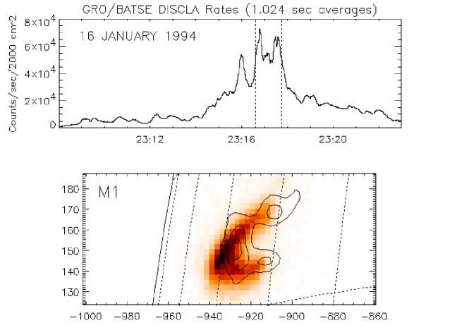
Figure 4.: Observations of the flare of 16 January 1994. a GRO/BATSE light curve (nominally 25-50 keV); b Yohkoh HXT image, 23-33 keV (isolines) and SXT image (gray scale).img:disk

2.2 Flares located on the solar disk

sec:disk

Usually, HXR footpoints sources are well seen in the case of flares located on the solar disk. It is more difficult to recognize HXR loop-top sources and to estimate their altitudes.

We have selected a sample of disk flares for which QPOs were observed and loop-top sources could be identified and measured (see example in Fig. img:disk). The distance, $D$, between the HXR footpoints has been taken for these flares as the measure of the loop size ($h=D/2$ for a semicircular loop). We have calculated wave velocity, $v_{1}$, for a whole loop as

$$v_{1}={\pi}D/P$$ (7)

and the corresponding magnetic field, $B_{1}$, from Eq. (3).

Next, we have calculated the values of $v_{2}$ and $B_{2}$ for the cusp-like model from Eqs. (4) and (5). The obtained values are given in Table tab2.

We see that Table tab2 confirms the properties seen in Table tab1. The values of $v_{1}$ and $B_{1}$ show large dispersion. The values of $v_{2}$ and $B_{2}$ show much smaller dispersion and they are in very good agreement with those in Table tab1. We consider this to indicate the advantage of the cusp-like model.

2.3 Investigation of sequences of HXR images

sec:seq

Important information can be derived from analysis of sequences of HXR images. Such a sequence for a flare of 16 January 1994 is shown in Fig. img:seq (Yohkoh 23-33 keV images). The location and structure of this flare are shown in Fig. img:disk. The loop-top (LT) and the footpoint (F1 and F2) sources are well seen in the images of Fig. img:seq. At the top of this figure is shown the HXR light curve with the time intervals for which the images Nos. 1-6 have been accumulated. Images Nos. 2, 4, and 6 correspond to the main HXR peaks and images Nos. 3 and 5 correspond to “valleys” between the peaks.

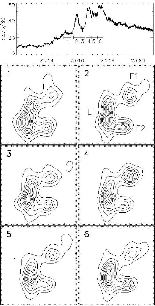
Figure 5.: Yohkoh 23-33 keV observations of the flare No 8 (of 16 January 1994). Top: the HXR light-curve. The HXR images (lower panels) have been accumulated for time intervals 1–6. See text for discussion.img:seq

Let us note that – in spite of moderate spatial resolution – a trace of a triangular structure of the HXR loop-top source is seen in images Nos. 1 and 3 of the figure. It is not seen during the maximal compression of the traps (images Nos. 4 and 6).

Figure tvar shows time-variation of the intensity of the brightest pixel in footpoints F1 and F2 and in loop-top source. We see that the main HXR peaks, Nos. 2, 4 and 6, are best seen in the footpoint intensity, but they are less marked in the loop-top intensity. This is in agreement with the outlined model: high energies of electrons are achieved at the end of trap compression and then they can easily escape towards the footpoints, so that their contribution to the loop-top emission is moderate.

Let us note that there is some asymmetry in time-variation of the footpoint intensity ($I_{1}>I_{2}$ at peak No. 4 and $I_{1}<I_{2}$ at peak No. 6). This indicates that there is some asymmetry in the oscillation of main trap (left-right oscillations in Fig. schemeb) which causes that the time variation of the ratio $\chi$ is somewhat different for the two ends of the trap.

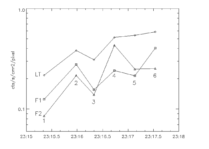
Figure 6.: Time-variation of the HXR intensity (23–33 keV) of the brightest pixel in the footpoints F1 and F2 and in the loop-top source.tvar

Similar results for other flares will be presented in another paper.

Hitherto we have considered impulses (peaks) of HXR emission. But it is important that HXR emission from the loop-top and footpoint sources is seen also during the HXR valleys (see Figs. img:seq-tvar). This means that the process of electron acceleration and precipitation is operating all the time during the impulsive phase, also during the HXR valleys. To explain this, let us return to Fig. schemeb. Beginning of intensive reconnection at P generates vigorous reconnection downflow which collides with the transverse magnetic field R and causes compression of a “main” magnetic trap and onset of its oscillations. But the reconnection is continued and this means that a sequence of magnetic traps, which are located above the main trap, undergo compression and can oscillate. The compression and oscillations of these traps are shifted in time relative to main trap, so that the acceleration and precipitation of the electrons occurs during the whole impulsive phase, including the HXR valleys. Hence, the HXR observations suggest that the cusp-like volume BPC is a dynamic region which is filled with moving, oscillating and colliding magnetic traps and it is the volume where electrons are accelerated.

If the main oscillating trap is a dominant one (i.e. it contains large number of particles), quasi-periodic sequence of HXR impulses will be observed. If, however, there are several oscillating traps of similar contribution to the HXR emission, the HXR peaks can be randomly (i.e. not quasi-periodically) distributed, as it is the case for impulsive phase of many flares.

tom01 investigated positions of HXR and SXR loop-top sources for limb flares, during their impulsive phase. He has found that in most cases the HXR and SXR sources are co-spatial or nearly cospatial. This result has been recently confirmed by k+l08 using RHESSI observations; see also tom09. These results indicate that in most cases both the HXR and SXR loop-top emission, recorded during the impulsive phase, comes from the same or nearly the same plasma volume. Let us note that this common volume of loop-top HXR and SXR sources confirms that HXR loop-top sources (like SXR ones) are also feeded by chromospheric evaporation upflows.

mas94 has found that in some flares the HXR loop-top source is located clearly above the SXR loop – see his flare of 13 January 1992 at 17:28 UT. The schematic diagram in Fig. cusp just concerns the “Masuda flare” of 13 January 1992.

In order to explain such cases as the Masuda flare we should take into account that in the BPC cusp volume there is a sequence of many moving traps and the dynamics of compression of individual traps is determined by the time variation of the velocity, $v(t)$, of reconnection outflow at the top of the cusp. The traps in the lower part of the cusp volume are “typical”: they undergo efficient compression, i.e. ${\chi}_{min}$ is low for these traps. HXR emission from these low traps was seen in the Yohkoh L-channel (14–23 keV) – see mas94. But these traps were not seen at higher energies ($E>20$ keV) because (1) the higher energies of electrons are achieved at the end of trap compression and then they can immediately precipitate toward the loop footpoints, (2) there was a dominant HXR ($E>20$ keV) sources at higher altitude. The heating of the footpoints causes filling of the loop with hot plasma and hence the loop is seen in SXRs. This description is confirmed by the fact that HXR footpoint sources were located just at the ends of the SXR loop (see Fig. 12.12 in asc04).

The enhanced HXR emission ($E>20$ keV) from the upper part of the cusp indicates that the compression of the traps located there is less efficient, so that the ratio $\chi$ remains high also during maximum of compression and hence the escape of accelerated electrons is more difficult (the traps are “semiclosed”). The accelerated electrons remain within the trap for longer time and they emit HXRs before they escape from the trap.

Hence, the main point of our interpretation of the Masuda flare is that the footpoint HXR sources are fed by the accelerated electrons coming from “typical” traps, which are situated low in the cusp volume BPC, and the top HXR source is a “semiclosed” magnetic trap, from which escape of particles is more difficult.

Our model can also easily explain the cases when HXR loop-top source is located below the SXR loop. Then “semiclosed” traps are located at the bottom of the BPC cusp volume, below the “typical” traps which are seen in SXRs. Such examples have been found by k+l08 and tom09. In their papers ${\Delta}h$ is the vertical distance between the centroids of HXR and SXR loop-top sources and ${\Delta}h<0$ means that the HXR source is located below the SXR one (see Fig. 2 in k+l08). Let us note that such cases cannot be easily explained by models which assume that a fast shock is formed within the BPC cusp volume (mas94, s+k97).

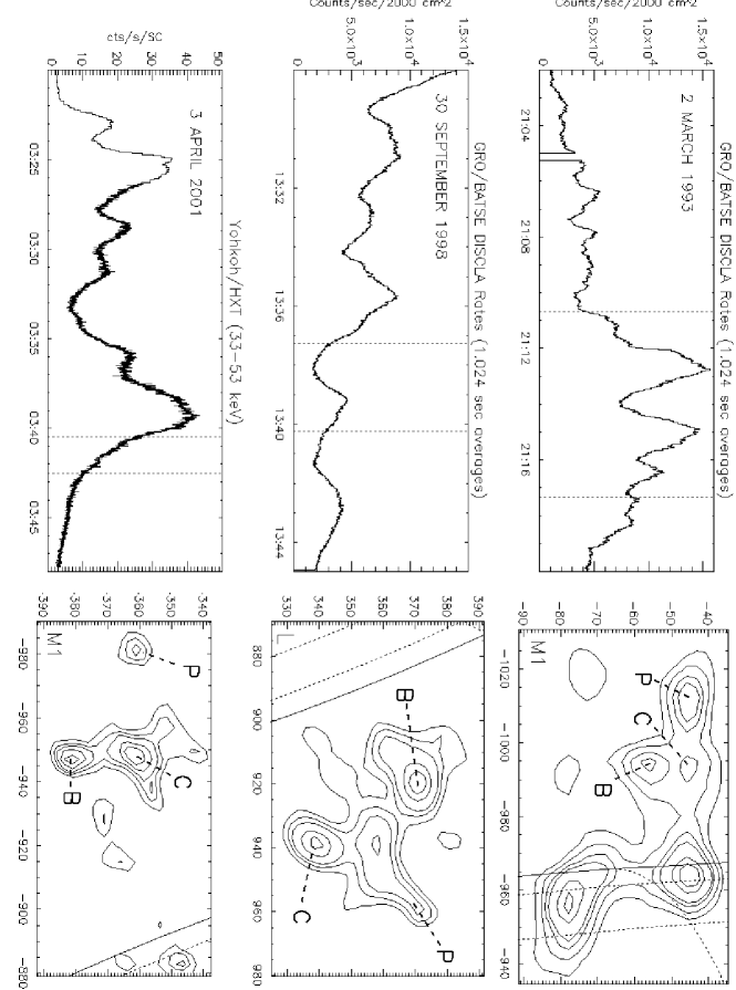
Figure 7.: Hard X-ray observations for three limb flares. Left: HXR light-curves (dashed vertical lines indicate accumulation times of the HXR images shown on the right). Right: Yohkoh HXR images of the flares. Solid line shows solar limb and dashed lines are on the solar disc.limb2

2.4 Limb flares with periods $P>120$ s

llimb

Table 3.: Limb flares with periods $P>120$ s^atab3

Flare	Date; time [UT]	$P$	$h$	$v_{1}$	$B_{1}$	$a$	$v_{2}$	$B_{2}$
No.		[s]	[Mm]	[km s-1]	[G]	[Mm]	[km s-1]	[G]
12	93/03/02; 21:10–21:15	(93); 137	38	1700	78	15	690	32
13b	98/09/30; 13:29–13:38	140; 166	38	1700	78	20	900	41
14b	01/04/03; 08:18–08:23	150; 206	34	1400	64	20	840	39

• Definition of parameters: $a$ is the size of cusp-like structure; $v_{2}=2{\pi}a/P$; the other parameters are the same as in Table tab1.

• Structure and evolution of these flares were investigated by bak07.

In this Section we consider three limb flares with periods $P>120$ s (Fig. limb2 and Table tab3). All they are high structures (see the altitudes, $h$, in Table tab3) and long-duration events (LDE). Yohkoh SXR observations were available for the flares Nos. 13 and 14. Their SXR images (grey scale) together with HXR isophotes are shown in Fig. limb:2ar. The SXR images show that they were big arcade flares.

In particular, very interesting is the large triangular structure seen in the HXR image of the flare No. 13 of 30 September 1998 (see Fig. limb2). The dominant HXR sources, B and C, are located at the altitude of SXR arcade (see Fig. limb:2ar). Weak HXR footpoint sources, located on the solar disc, are better seen in Yohkoh M1 (23-33 keV) and M2 (33-53 keV) images.

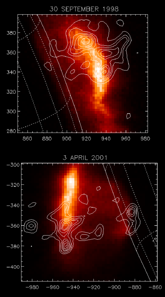
Figure 8.: Soft X-ray images of the flares Nos. 13 and 14 (gray scale). The isophotes show HXR images like in Fig. limb2: it is 14-23 keV image in the case of 30 September 1998 flare and 23-33 keV image for the 3 April 2001 flare.limb:2ar

We have assumed that this triangular structure is analogous to BPC cusp-like structure in Fig. scheme where the observed oscillations occur. The two dominant HXR sources, B and C, correspond to the magnetic mirrors, B and C, in Fig. scheme. Charged particles spend somewhat longer time (calculated per unit length along the magnetic trap) near the magnetic mirrors than in other parts of the trap and therefore the HXR emission is enhanced near the mirrors. The enhanced emission near P and along the line running downwards from P, is due to the fact that plasma density is somewhat higher there because of reconnection stream flowing from the current sheet at P. The higher density increases the HXR emissivity.

We have taken the distance, $a$, between the top source P and the line connecting B and C, as the height of the cusp structure, and calculated the velocity $v_{2}$ as

$$v_{2}=\frac{2{\pi}a}{P}$$ (8)

and then the magnetic field strength $B_{2}$ from Eq. (5). The values of $v_{1}$ and $B_{1}$ calculated from Eqs. (1) and (3), as well as $v_{2}$ and $B_{2}$ are given in Table tab3.

Flare No. 14 of 3 April 2001 is a similar case. It was also a large arcade flare and the sources B and C were located at the altitude of SXR arcade. A top HXR source P is seen in Yohkoh M1 (23–33 keV) images which confirms that this is also a similar triangular HXR structure. HXR footpoint sources are seen on the solar disc, but they are weaker than the B and C sources. Again, we have measured the height of the cusp structure as the distance between the top source P and the line connecting B and C and the obtained values of $v_{1}$, $B_{1}$, $v_{2}$, and $B_{2}$ are given in Table tab3.

Our model (connection of sources B and C by a cusp-like structure like in Fig. schemeb) explains why in flares Nos. 13 and 14 the sources B and C are similar in intensity and their time evolution is similar. Figure limb:2ar indicates that in the both flares the plane BPC of the cusp-like structure is not perpendicular to the arcade axis. This can be due to the shear in footpoint motion at the photosphere (see Fig. 3.10 in pri87). The sources B and C are located at the places where cusp-like magnetic lines meet the arcade loops (the places are located on the opposite sides of the arcade axis).

No SXR images were available for the flare No. 12 of 2 March 1993. In the HXR image of this flare (Fig. limb2) strong footpoint sources are seen on the solar disc and a triangular structure BPC is seen at the top. The strong footpoint emission indicates that the oscillations of magnetic traps were more dynamic (low value of ${\chi}_{min}$) and therefore the accelerated electrons could easily escape towards the footpoints. We have measured the altitude, $h$, and the height, $a$, of the cusp-like structure at the top and obtained values of $v_{1}$, $B_{1}$, $v_{2}$, and $B_{2}$ are given in Table tab3.

In Table tab3 we see that the values of $v_{2}$ and $B_{2}$ are similar to those obtained for flares with periods 10–60 s (Tables tab1 and tab2). This supports our assumption that the large triangular HXR structures, considered in this Section, are large magnetic cusp-like structures.

3 Discussion

sec:disc

A lower limit for the Alfven speed can be estimated as follows:

$$v_{A}=2.2\times 10^{11}B/\sqrt{N}\quad\mbox{[cm\,s${}^{-1}$]}\quad$$ (9)

where $N$ is the electron density. For a magnetic trap it should be

$$B^{2}/(8\pi)>2NkT,$$ (10)

where $k$ is the Boltzmann constant and $T$ is the temperature. This gives

$$B/\sqrt{N}>8.3\times 10^{8}\sqrt{T}$$ (11)

Hence the lower limit for the Alfven speed is [Eqs. (9) and (11)]:

$$v_{A}>1.8\times 10^{4}\sqrt{T}\quad\mbox{[cm\,s${}^{-1}$]}\quad$$ (12)

Taking $T>10^{7}$ K for the temperature in the trap, we obtain

$$v_{A}>5.7\times 10^{7}\quad\mbox{cm\,s${}^{-1}.$}\quad$$ (13)

We see in Tables tab1–tab3 that our estimates of the Alfven speed, $v_{2}$, are higher than this lower limit, but they are not much higher. This means that the magnetic pressure, $B^{2}/(8\pi)$, is not much higher than the gas pressure, $p$, in the acceleration volume. This is important for MHD modeling of flaring loops.

In Fig. plot the diameter, $d$, of the HXR loop-top source is plotted vs. the oscillation period, $P$. For short periods, $P=10-60$ s, good correlation between $d$ and $P$ is seen. [A diagram displaying $h$ (or $D$/2) vs. $P$ shows much larger dispersion.] This is a confirmation that the investigated oscillations occur in confined magnetic structures displayed as the HXR sources. This supports our model of the oscillations of magnetic traps in cusp-like magnetic structures.

Figure 9.: Correlation between the HXR loop-top source diameter, $d$, and the oscillation period, $P$. For large sources ($P>120$ s) the values of $2a$ were taken for $d$ – see text. Point marked with a square relates to the flare investigated by Ofman & Sui (2006). The larger cross at the first data point on the left shows r. m. s. error bars which concern all small HXR sources, $P<60$ s, marked with small crosses.plot

For the large HXR sources ($P>120$ s), the values of $2a$ were taken instead of $d$ in Fig. plot, where $a$ is the height of a triangular HXR structure. It appears that the large HXR structures also fit the correlation between $d$ and $P$ determined by the small structures. This supports our assumption that the large triangular HXR structures are the cusp-like magnetic structures in which the oscillations with period $P>120$ s occur.

o+s06 have analyzed RHESSI observations of QPOs in a flare of 19 January 2005 with period $P\simeq 150$ s. We have measured the size, $a$, of the HXR loop-top source in the same manner as for our three large Yohkoh flares and we have plotted additional point marked with a square in our test diagram in Fig. plot. We see that this additional flare fits quite well into our model of oscillating magnetic traps.

It may be important that all four large flares in Fig. plot have periods about 140–150 s, which suggests that they may be overtones of the 300 s solar oscillations. This would mean that the oscillations are maintained due to a resonance with the 300 s oscillations. In particular, this seems to be probable in the case of our flares Nos. 13 and 14 and the flare investigated by o+s06, in which the HXR oscillations are quasi-sinusoidal (not typical sequences of increasing impulses like in Fig. lc).

For a number of flares mar06 has found decaying oscillations of periods 5.5$\pm$2.7 minutes in Doppler shifts of SXR spectral lines. He explained them as being due to slow-mode or fast magnetosonic oscillations of whole flaring loops. We have investigated Yohkoh HXR records for those flares and we have found no counterpart of the Mariska’s oscillations in the HXRs. Mariska’s flares were rather small, hence the observed oscillations most probably were the relaxation oscillations of whole flare magnetic structure which were excited by collision of violent chromospheric evaporation upflows. Moreover, for some Mariska’s flares we have found HXR quasi-periodic oscillations of period 10–60 s analogous to those investigated in the present paper. This is an additional indication that the HXR oscillations with periods 10–60 s occur in smaller volumes and they are different from the longer-period oscillations observed by Mariska. These cases will be investigated in a separate paper.

Important information can be obtained from CGRO/BATSE observations due to their high sensitivity in HXRs. An example of such observations is shown in Fig. img:disk (upper panel). We see that a sequence of weak quasi-periodic impulses began about 23:09 UT, but a typical impulsive phase began about 23:14 UT. (Similar weak oscillations before the impulsive phase are seen in flare of 2 March 1993 in Fig. limb2). These observations are in agreement with the model of oscillating traps: The oscillations began about 23:09 UT. Accelerated particles hit the footpoints and chromospheric evaporation begin.

The plasma moves along the same magnetic lines, connecting traps with footpoints, and about 23:14 UT it reaches the oscillating traps. During the expansion of a trap this plasma fills the trap and therefore a larger number of electrons will be accelerated during the next compression of the trap. Hence, there is now a feedback between the number of accelerated electrons and the density of the plasma which reaches the traps. This feedback causes that the HXR intensity increases with time, as it is seen in Fig. img:disk.

Hence, the model of oscillating magnetic traps provides a simple explanation of the well-known paradox that the number of electrons, which are accelerated during big flares, is much higher than it can be provided by surrounding corona.

Let us repeat that, according to discussion of Fig. img:disk, chromospheric evaporation begins a few minutes before the beginning of the impulsive phase. The beginning of the evaporation causes increase of the SXR emission. Hence, the model of electron acceleration in oscillating magnetic traps is in agreement with the well-known fact that SXR emission of a flare usually begins a few minutes before the beginning of HXR impulsive phase.

Thermal conduction also contributes to the energy transport from the loop top to its footpoints during the impulsive phase and it increases the rate of chromospheric evaporation.

Our model of oscillating magnetic traps explains very well why the time intervals, $P$, between the HXR impulses are not equal. The oscillations occur in a volume of changing magnetic field and plasma density, so that the Alfven speed can change from one pulse to another.

Figure 10.: HXR light curve (nominally 25-50 keV) for the flare of 14 May 1993 (flare No. 6).lc

In the present paper we have considered a cusp-like magnetic configuration. We see from this example that two factors are necessary for magnetic-trap compression and excitation of their oscillations: a magnetic-field reconnection and an obstacle (a transverse magnetic field) on the way of the reconnection flow. But the location and orientation of the reconnection site can be different in different flares.

Let us note that our model of exciting oscillations of magnetic traps is similar to that proposed for oscillations during onset of magnetospheric substorms. The substorm begins with a violent reconnection in the magnetospheric tail (see observations presented by nak04). The reconnection outflow directed Earthward collides with the inner (dipole-like) magnetic field, causes magnetic field compression and excitation of oscillations. An example of magnetic field oscillations during the onset of a substorm is shown in Fig. sstorm (a smooth substorm variation of the magnetic field has been removed from these records). We see a short sequence of oscillations which is similar to what we see in HXRs of investigated flares (the smooth variation of HXR intensity was not removed from our light curves).

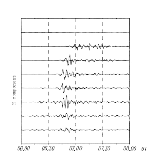
Figure 11.: Magnetic field oscillations during the onset of a geomagnetic substorm of 23 November 1970 (smooth variation has been removed) as recorded by seven geomagnetic stations in Canada. The distance between the horizontal lines amounts to 316 $\gamma$. From Nishida (1978).sstorm

4 Summary and conclusions

concl

We have investigated flares for which quasi-periodic HXR oscillations and HXR loop-top sources were clearly seen. Our analysis has shown that the observed HXR oscillations are confined within the loop-top sources. This is supported by a correlation between the periods, $P$, and the sizes, $d$, of the loop-top sources.

mar06 has found that oscillations of whole flaring loops had periods of 5.5$\pm$2.7 minutes. Recently we have found that HXR oscillations with periods $P=10-60$ s occurred in some of the Mariska’s flares which confirms that the oscillations seen in HXRs, occurred in smaller magnetic structures (these results will be presented in a separate paper).

We have argued that a model of oscillating magnetic traps is adequate to describe the HXR observations. During the compression of a trap particles are accelerated, but during its expansion plasma coming from chromospheric evaporation, fills the trap. This feedback between the particle acceleration and filling of the traps explains high number of electrons which are accelerated in strong flares. This model is clearly supported by finding weak HXR oscillations a few minutes before the impulsive phase (see Sect. sec:disc).

We have estimated the mean strength of the magnetic field inside the oscillating traps. It amounts to about 30–40 Gauss, which is lower than assumed in other papers (see asc04).

We have compared the properties of the HXR oscillations with available models of flare magnetic structure and particle acceleration and indicated the most adequate scenario (see Sections obs and sec:disc).

HXR light curves can be divided into two components (see asc96, tom01): a smooth component (a smooth line connecting valleys) and impulsive one (increases above the smooth line). The smooth component is the result of continuous acceleration in many traps whose oscillations are shifted in phase (this is due to continuous reconnection at the top of cusp structure). The increase of the smooth component during the impulsive phase (like in Fig. lc) is parallel to increase of the SXR loop-top emission which confirms that the increase of the smooth HXR component is also due to the increase of the density within the cusp-like volume.

If there is a pronounced maximum in the time-profile of the reconnection rate at the top of cusp, then a dominant (large) trap will be generated within the cusp-like volume and its oscillations will be seen as quasi-periodic oscillations in HXRs.

We have pointed out that in most cases the HXR and SXR sources are cospatial or overlap during the impulsive phase which confirms that both emissions come from the common cusp-like plasma volume. But in seldom cases the HXR and SXR loop-top sources are clearly separated (like in “Masuda flare”). We explain such cases of HXR sources as being due to magnetic traps, for which the ratio $\chi$ remains high during the compression, so that accelerated electrons remain there for a longer time and therefore generate enhanced HXR emission. This explanation is also important for the flares having weak HXR footpoint emission (like in the case of v+b04).

In our paper of 1998 Jakimiec et al. (1998) we have found that (a) loop-top flare kernels are multithermal, (b) significant random motions occur in the kernels. On this basis we have proposed that the kernels are filled with MHD turbulence. In the present paper we have used observations of HXR oscillations to improve the model of loop-top kernels. We have come to the conclusion that during the impulsive phase the kernels are filled with oscillating magnetic traps. The oscillations are excited and maintained by violent reconnection flow. The advantages of this model are the following: (1) it incorporates a simple model of particle acceleration (Fermi and betatron acceleration), (2) the particles can easily escape after their acceleration. We will observe this plasma volume as being “turbulent” (random motions due to oscillations shifted in phase; temperature differences between different traps). (We think that MHD turbulence can develop later on due to collision of chromospheric evaporation upflows. This would ensure long duration of the kernels.)

Acknowledgements

The Yohkoh satellite is a project of the Institute of Space and Astronautical Science of Japan. The Compton Gamma Ray Observatory is a project of NASA. The authors are thankful to Dr. Urszula Bak-Ste$\acute{\rm{s}}$licka for her help in selecting appropriate flares. This work was supported by Polish Ministry of Science and High Education grant No. N N203 1937 33.

References

- Asai et al. (2004) Asai, A., Yokoyama, T., Shimojo, M., & Shibata, K. 2004, ApJ605, L77
- Aschwanden (2004) Aschwanden, M. J. 2004, Physics of the Solar Corona. An Introduction, Springer: Praxis
- Aschwanden et al. (1996) Aschwanden, M. J., Wills, M. J., Hudson, H. S., Kosugi, T., Schwartz, R. A. 1996, ApJ468, 398
- Bak-Stelicka (2007) Bak-Stelicka, U. 2007, Ph. D. thesis, University of Wrocław
- Bogachev & Somov (2005) Bogachev, S. A., & Somov, B. V. 2005, Astron. Letters 31, 537
- Foullon et al. (2005) Foullon, C., Verwichte, E., Nakariakov, V. M., & Fletcher, L. 2005, A&A440, L59
- Jakimiec (2002) Jakimiec, J. 2002, in Wilson E. (ed.), Proc. of the 10th European Solar Physics Meeting, Solar Variability: From Core to Outer Frontiers, ESA SP-506, 645
- Jakimiec (2005) Jakimiec, J. 2005, in Danesy, D., Poedts, S., De Groof, A., Andries, J. (eds.), Proc. of the 11th European Solar Physics Meeting, The Dynamic Sun: Challenges for Theory and Observations, ESA SP-600, 124.1
- Jakimiec et al. (1998) Jakimiec, J., Tomczak, M., Falewicz, R., Phillips, K. J. H., & Fludra, A. 1998, A&A334, 1112
- Karlick & Kosugi (2004) Karlick, M., & Kosugi T. 2004, A&A419, 1159
- Kołomaski (2007) Kołomaski, S. 2007, A&A465, 1021
- Krucker & Lin (2008) Krucker, S., & Lin, R. P. 2008, ApJ673, 1181
- Lipa (1978) Lipa, B. 1978, Sol. Phys.57, 191
- Mariska (2006) Mariska, J. T. 2006, ApJ639, 484
- Masuda (1994) Masuda, S. 1994, Ph. D. thesis, University of Tokyo
- Nakamura (2004) Nakamura, R. 2004, ESA Bulletin 118, 64
- Nakariakov et al. (2006) Nakariakov, V. M., Foullon, C., Verwichte, E., & Young, N. P. 2006, A&A452, 343
- Nishida (1978) Nishida, A. 1978, Geomagnetic Diagnosis of the Magnetosphere, Physics and Chemistry in Space, New York: Springer
- Ofman & Sui (2006) Ofman, L., & Sui, L. 2006, ApJ644, L149
- Priest (1987) Priest, E. R. 1987, Solar Magnetohydrodynamics, D. Reidel Publishing Company
- Sato et al. (2006) Sato, J., Matsumoto, Y., Yoshimura, K., et al. 2006, Sol. Phys.236, 351
- Somov & Kosugi (1997) Somov, B. V., Kosugi, T. 1997, ApJ485, 859
- Spitzer (1962) Spitzer, L. 1962, The Physics of Fully Ionized Gases, Interscience, New York
- Tomczak (1997) Tomczak, M. 1997, A&A317, 223
- Tomczak (2001) Tomczak, M. 2001, A&A366, 294
- Tomczak (2009) Tomczak, M. 2009, A&A502, 665
- Veronig & Brown (2004) Veronig, A. M., & Brown, J. C. 2004, ApJ603, L117