Persistence effects in deterministic diffusion

Abstract

In systems which exhibit deterministic diffusion, the gross parameter dependence of the diffusion coefficient can often be understood in terms of random walk models. Provided the decay of correlations is fast enough, one can ignore memory effects and approximate the diffusion coefficient according to dimensional arguments. By successively including the effects of one and two steps of memory on this approximation, we examine the effects of “persistence” on the diffusion coefficients of extended two-dimensional billiard tables and show how to properly account for these effects, using walks in which a particle undergoes jumps in different directions with probabilities that depend on where they came from.

I Introduction

Diffusion is a fundamental macroscopic phenomenon in physical systems, which, for instance, characterizes the spreading of tracer particles in a solvent. At a mescoscopic scale, it can be traced to the cumulative effect of many “random” displacements, as in Brownian motion Cha43 . At the underlying microscopic scale, however, the dynamics of a system are deterministic. Deterministic diffusion concerns the study of microscopic models whose deterministic dynamics also exhibit diffusive behavior at a macroscopic scale Gas98 ; Dor99 ; Kla07 .

A particularly appealing, physically motivated model which does exhibit this phenomenon is the periodic Lorentz gas BS80 . Here, independent point particles in free motion undergo elastic collisions with fixed hard disks in a periodic array. The diffusive motion can then be considered to be a result of the chaotic nature of the microscopic dynamics, according to which nearby initial conditions separate exponentially fast due to the convex nature of the obstacles. Thus a cloud of (non-interacting) particles in this Lorentz gas spreads out over time in a way similar to that of solutions of the diffusion equation,

$$\left\langle[\mathbf{x}(t)-\mathbf{x}(0)]^{2}\right\rangle\sim 4Dt,$$ (1)

where $\mathbf{x}(t)$ denotes the position of a tracer at time $t$, with initial position $\mathbf{x}(0)$, and the mean squared displacement is computed as an average $\left\langle\cdot\right\rangle$ over many realizations of this process. The diffusion coefficient, $D$, is a constant which depends on the geometrical parameters of the system, i.e., the underlying microscopic dynamics.

The diffusion coefficient summarizes the macroscopic behavior of the system while capturing the microscopic properties of the dynamics that lead to it. A central question in deterministic diffusion is to understand how this dependence on the geometrical parameters comes about. This has been addressed in particular by Machta and Zwanzig MZ83 , who showed that in the limit where the obstacles are close together, the motion reduces to a stochastic Bernoulli-type hopping process—a random walk—between “traps”. By calculating the diffusion coefficient of this random walk, they were able to obtain a reasonable agreement with the numerically-measured value of the diffusion coefficient.

The approach of Machta and Zwanzig was extended heuristically by Klages and Dellago KD00 , by including important physical effects not taken into account in the simple random-walk picture, namely a possibly non-isotropic probability of changing directions, and of crossing two traps at once. Klages and Korabel KK02 then provided an alternate approach, in which they employed a Green-Kubo expansion of the diffusion coefficient to obtain a series of increasingly accurate approximations, based on numerically-calculated multi-step transition probabilities. In one particular Lorentz gas model, they showed that their results are in good agreement with this expansion, see also Kla07 . Nonetheless, as we emphasize below, the physical motivation, and indeed the physical meaning, of this approach, are not clear.

The purpose of this paper is to show that in fact the correct expansion beyond the Machta-Zwanzig approximation is to incorporate this type of correction in the framework of persistent random walks. In other words, to be consistent, memory effects of a given length, whether one or several steps, must be accounted for through their contribution at all orders in the Green-Kubo formula relating the diffusion coefficient to the velocity auto-correlations. This is physically strongly motivated, and provides the correct way of incorporating correlation effects, in principle, of any finite order.

In the usual periodic Lorentz gas on a triangular lattice considered in KK02 , the model is sufficiently isotropic that higher order contributions are small and can be safely neglected. However, when the correlation effects are very strong, this is no longer the case. We introduce a billiard model with this property and show that, whereas a Green-Kubo–type expansion fails except very close to the Machta-Zwanzig limiting case, the approximation based on a first-order persistent random walk is in reasonable agreement with the data. By further considering memory effects up to two successive steps, we find that the agreement between the numerically-measured diffusion coefficient of the billiard table and that of the second-order persistent random walk extends to an appreciably larger range of parameters.

II Periodic Lorentz gas on a triangular lattice

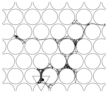
Figure 1: Periodic Lorentz gas on a triangular lattice. A typical trajectory is shown, which starts at the upper right disk in the initial cell—marked by the highlighted triangle—and moves across the table, performing a diffusive motion.

Consider the periodic Lorentz gas on a triangular lattice, shown in Fig. 1. The centers of three nearby disks are identified as the vertices of equilateral triangles which, in our notation, will be taken to be of unit side length. Denoting by $\rho$ the radius of the disks, we let $\delta\equiv 1-2\rho$ denote the spacing between disks. When $\delta=0$, the triangles form closed traps from which the tracer particles cannot escape. If, however, $0<\delta\ll 1$, then we expect the particles to remain inside the cell for a long time before they can escape to another cell. This argument can be made precise using ergodic theory MZ83 . Given a tracer of unit velocity, the mean trapping time $\tau$ is given in terms of the ratio of the cell area to the lengths of the holes by CM06

$$\tau=\pi\frac{\sqrt{3}/4-\pi\rho^{2}/2}{3\delta}=\pi\frac{\sqrt{3}/4-\pi(1-\delta)^{2}/8}{3\delta}\,.$$ (2)

Assuming that this time is longer than the typical decay of correlations , Machta and Zwanzig MZ83 argued that the diffusion coefficient of the Lorentz gas can be approximated by a memory-less random walk (called the “short-memory approximation” in Z83 ),

$$D_{\mathrm{MZ}}=\frac{\ell^{2}}{4\tau}\,,$$ (3)

where, in our notation, the lattice spacing $\ell=1/\sqrt{3}$.

Taking further account of memory effects, Klages & Korabel KK02 noted that the Machta-Zwanzig approximation (3) is the zeroth order expansion of a series given by the Green-Kubo formula for the diffusion coefficient:

$$D=D_{\mathrm{MZ}}\left(1+2\sum_{k=1}^{\infty}\left\langle\mathbf{v}_{0}\cdot\mathbf{v}_{k}\right\rangle\right),$$ (4)

where $\mathbf{v}_{k}$ is the jump vector (“velocity”) between traps on the $k$th step, and $\left\langle\mathbf{v}_{0}\cdot\mathbf{v}_{k}\right\rangle$ are auto-correlations of the velocity at steps $0$ and $k$.

The approach taken in KK02 was to truncate the expression (4) at a finite value of $k$, assuming that all higher-order correlations are $0$. They showed that by numerically calculating the terms appearing in this equation, the results evaluated by this truncation converged to the numerically-obtained diffusion coefficient.

However, this ad hoc truncation has no physical meaning: if $\left\langle\mathbf{v}_{0}\cdot\mathbf{v}_{1}\right\rangle\neq 0$, it is not true that higher-order correlations $\left\langle\mathbf{v}_{0}\cdot\mathbf{v}_{k}\right\rangle$ vanish. Rather, assuming that the process has memory of the previous step alone—which we will refer to as the single-step memory approximation—one must compute the correlations $\left\langle\mathbf{v}_{0}\cdot\mathbf{v}_{k}\right\rangle$ in a consistent way, and evaluate the diffusion coefficient (4) by taking all the $k$’s into consideration.

II.1 Single-step memory approximation

The process for which the motion of a particle at step $k+1$ depends explicitly on the state at step $k$ is known as a persistent or correlated random walk WR83 ; Hu95 ; HK87 ; We94 . The technique for studying such walks is well developed, and consists of treating it as a random walk with internal states, which, in this case, describe the direction with which the walker arrives at a site.

Considering a persistent random walk on a honeycomb lattice, we denote by $P_{\mathrm{b}}$ the conditional probability to return in the direction opposite to the current one, $P_{\mathrm{r}}$ to turn right and $P_{\mathrm{l}}$ to turn left. In terms of these quantities, the velocity auto-correlation is found to be GS09

$$\left\langle\mathbf{v}_{0}\cdot\mathbf{v}_{k}\right\rangle = \frac{(-1)^{k}}{2}\Bigg{\{}\left[P_{\mathrm{b}}-\frac{P_{\mathrm{r}}+P_{\mathrm{l}}}{2}-i\frac{\sqrt{3}}{2}(P_{\mathrm{r}}-P_{\mathrm{l}})\right]^{k}$$ (5)

$$+\left[P_{\mathrm{b}}-\frac{P_{\mathrm{r}}+P_{\mathrm{l}}}{2}+i\frac{\sqrt{3}}{2}(P_{\mathrm{r}}-P_{\mathrm{l}})\right]^{k}\Bigg{\}}\,,$$

where $i=\sqrt{-1}$. In the case of a symmetric walk for which $P_{\mathrm{r}}=P_{\mathrm{l}}\equiv P_{\mathrm{s}}=(1-P_{\mathrm{b}})/2$, the diffusion coefficient (4) is

$$D_{\mathrm{1SMA}}=D_{\mathrm{MZ}}\frac{3(1-P_{\mathrm{b}})}{1+3P_{\mathrm{b}}}\,.$$ (6)

In comparison, the first order approximation made in KK02 is to write

$$D^{(1)}_{\mathrm{KK}}=1+2\left\langle\mathbf{v}_{0}\cdot\mathbf{v}_{1}\right\rangle=D_{\mathrm{MZ}}(2-3P_{\mathrm{b}})\,,$$ (7)

which corresponds to the first-order approximation of Eq. (6) when expanding $D_{\mathrm{1SMA}}$ about the isotropic process for which $P_{\mathrm{b}}=1/3$.

II.2 Two-step memory approximation

For a persistent process with two-step memory approximation, there are nine conditional transition probabilities, which we denote by $P_{\mathrm{bb}}$, $P_{\mathrm{br}}$, $P_{\mathrm{bl}}$, $P_{\mathrm{rb}}$, $P_{\mathrm{rr}}$, $P_{\mathrm{rl}}$, $P_{\mathrm{lb}}$, $P_{\mathrm{lr}}$ and $P_{\mathrm{ll}}$, where, for instance, $P_{\mathrm{br}}$ denotes the probability that the tracer first moves backwards and then turns right, and similarly for the other symbols. Although the corresponding Markov chain involves a $9\times 9$ stochastic matrix, there are symmetries in the system which can be exploited to reduce the computations to $3\times 3$ matrices involving the transition probabilities listed above. The computation of the velocity auto-correlation then yields GS09

$$\langle\mathbf{v}_{0}\cdot\mathbf{v}_{k}\rangle=(-1)^{k}\frac{3}{2}\Big{(}1\enspace 1\enspace 1\Big{)}\left[\left(\begin{array}[]{c@{\enspace}c@{\enspace}c}P_{\mathrm{bb}}&P_{\mathrm{lb}}&P_{\mathrm{rb}}\\ \phi P_{\mathrm{bl}}&\phi P_{\mathrm{ll}}&\phi P_{\mathrm{rl}}\\ \phi^{2}P_{\mathrm{br}}&\phi^{2}P_{\mathrm{lr}}&\phi^{2}P_{\mathrm{rr}}\end{array}\right)^{k-1}\left(\begin{array}[]{c@{\enspace}c@{\enspace}c}1&0&0\\ 0&\phi&0\\ 0&0&\phi^{2}\end{array}\right)+\left(\begin{array}[]{c@{\enspace}c@{\enspace}c}P_{\mathrm{bb}}&P_{\mathrm{lb}}&P_{\mathrm{rb}}\\ \phi^{2}P_{\mathrm{bl}}&\phi^{2}P_{\mathrm{ll}}&\phi^{2}P_{\mathrm{rl}}\\ \phi P_{\mathrm{br}}&\phi P_{\mathrm{lr}}&\phi P_{\mathrm{rr}}\end{array}\right)^{k-1}\left(\begin{array}[]{c@{\enspace}c@{\enspace}c}1&0&0\\ 0&\phi^{2}&0\\ 0&0&\phi\end{array}\right)\right]\left(\begin{array}[]{c}p_{1}\\ p_{2}\\ p_{3}\end{array}\right)\,,$$ (8)

where $\phi=\exp(2i\pi/3)$ and $(p_{1},p_{2},p_{3})$ are the first three components of the stationary distribution of the Markov chain, which, for a left-right symmetric process for which $P_{\mathrm{rr}}=P_{\mathrm{ll}}\equiv P_{\mathrm{ss}}$, $P_{\mathrm{rb}}=P_{\mathrm{lb}}\equiv P_{\mathrm{sb}}$ and $P_{\mathrm{rl}}=P_{\mathrm{lr}}=1-P_{\mathrm{ss}}-P_{\mathrm{sb}}$, read

$$p_{1}=\frac{P_{\mathrm{sb}}}{3-3P_{\mathrm{bb}}+3P_{\mathrm{sb}}},\quad p_{2}=p_{3}=\frac{1-P_{\mathrm{bb}}}{6-6P_{\mathrm{bb}}+6P_{\mathrm{sb}}}.$$ (9)

The corresponding diffusion coefficient (4) is

$$D_{\mathrm{2SMA}}=D_{\mathrm{MZ}}\frac{3(1-P_{\mathrm{bb}})(1+P_{\mathrm{bb}}-P_{\mathrm{sb}})(2-P_{\mathrm{sb}}-2P_{\mathrm{ss}})}{(1-P_{\mathrm{bb}}+P_{\mathrm{sb}})[P_{\mathrm{sb}}(7+P_{\mathrm{bb}}-8P_{\mathrm{ss}})+2(1+P_{\mathrm{bb}})P_{\mathrm{ss}}-4P_{\mathrm{sb}}^{2}]}\,.$$ (10)

This compares to the second-order approximation following the truncation scheme in KK02 ,

$$D^{(2)}_{\mathrm{KK}} = D^{(1)}_{\mathrm{KK}}+2\left\langle\mathbf{v}_{0}\cdot\mathbf{v}_{2}\right\rangle\,,$$ (11)

$$= D_{\mathrm{MZ}}\frac{5-5P_{\mathrm{bb}}-7P_{\mathrm{sb}}+9P_{\mathrm{bb}}P_{\mathrm{sb}}}{2-2P_{\mathrm{bb}}+2P_{\mathrm{sb}}}\,.$$

We note that this expression is actually different from that given in KK02 , where the stationary distribution (9) was erroneously assumed to be uniform.

II.3 Numerical results

The transition probabilities of the single- and two-step memory approximation random walks can be computed for the Lorentz gas by estimating the relative frequencies of the corresponding events and taking into consideration the left-right symmetry of these transitions. Plugging their values into Eqs. (6) and (10), we obtain the corresponding coefficients and compare them to the diffusion coefficient of the billiard calculated from direct numerical simulations of the billiard dynamics. These results are shown in Fig. 2, including the results of the truncations (7) and (11).

In the limit $\delta\to 0$, we see that the Machta-Zwanzig approximation (3) is recovered. Looking at a broader range of parameter values, whereas the single-step approximation yields a good estimate of the actual diffusion coefficient of the Lorentz gas only for values of $\delta\lesssim 10^{-3}$, the extent of the range of validity of the two-step approximation is much larger, $\delta\lesssim 0.1$.

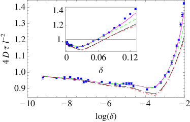
Figure 2: Numerical computation of the diffusion coefficient of the periodic Lorentz gas on a triangular lattice, here divided by the dimensional factor, Eq. (3). The lines correspond to the different approximate results discussed above: (long-dashed, black line) single-step memory approximation (6); (dot-dashed, red line) first-order truncation (7); (solid, magenta line) two-step memory approximation (10); (dashed green) second-order truncation (11).

As seen in the figure, the successive approximations (6) and (10) are slightly better than their respective counterparts (7) and (11). The differences between the results of Eqs. (6) and (7) on the one hand, and Eqs. (10) and (11) on the other hand are, however, quite small and not everywhere easy to appreciate. The reason is that the transition probabilities are nearly isotropic for all values of $\delta$ in the range of allowed values, viz. $\sqrt{3}/4<\delta<1/2$ (the lower bound corresponds to the finite-horizon condition). This fact, which we illustrate in Fig. 3 for the transition probabilities of the single-step memory approximation, explains the validity of the Klages–Korabel truncation scheme in this case.

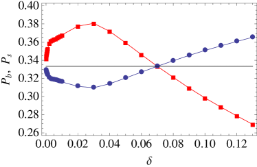
Figure 3: (Color online) Numerical computation of the transition probabilities $P_{\mathrm{b}}$ (squares) and $P_{\mathrm{s}}$ (circles) of the single-step memory approximation associated to the periodic Lorentz gas on a triangular lattice. Similar results were reported in KD00 .

III Billiard table on a square lattice

In order to better emphasize the validity of our approximation scheme over simpler truncation methods, we turn to a class of billiard tables such as shown in Fig. 4, which alternates small and large disks on a square lattice. By inserting rigid horizontal and vertical barriers between the small disks, with gaps of size $\delta$ in their centers, we introduce a control parameter of relevance to the dynamical properties of the model which is independent of the other system parameters. However large the gaps, the trajectories in these billiards can be reconstructed from the trajectories of the same billiard with a single unit cell on the torus.

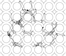
Figure 4: Periodic Lorentz table on a square lattice. A typical trajectory is shown, with the initial position marked by a thick dot. We take the inner and outer radii to be respectively $\rho_{\mathrm{i}}=0.36\ell$ and $\rho_{\mathrm{o}}=0.15\ell$ and vary only the size of the gaps.

The geometry of the lattice is such that the distance between neighboring disks is equal to the lattice spacing, which we take to be unity, $\ell=1$. Given the radii $\rho_{\mathrm{i}}$ of the large disks and $\rho_{\mathrm{o}}$ of the small disks, the trapping time is

$$\tau=\pi\frac{1-\pi(\rho_{\mathrm{i}}^{2}+\rho_{\mathrm{o}}^{2})}{4\delta}\,.$$ (12)

Given these two parameters, the Machta-Zwanzig approximation is here again given by Eq. (3). Note that in the present model, $D_{\mathrm{MZ}}$ depends linearly on $\delta$, contrary to the Lorentz gas discussed in the previous section, for which the area of the cells varied with $\delta$.

III.1 Single-step memory approximation

Consider a persistent random walk with single-step memory on a square lattice. We denote by $P_{\mathrm{f}}$, $P_{\mathrm{r}}$, $P_{\mathrm{b}}$ and $P_{\mathrm{l}}$, respectively, the conditional probabilities that the particle proceeds in the same direction, turns right, reverses direction, or turns left. The velocity auto-correlation is

$$\left\langle\mathbf{v}_{0}\cdot\mathbf{v}_{k}\right\rangle=\frac{1}{2}\{[P_{\mathrm{f}}-P_{\mathrm{b}}-i(P_{\mathrm{r}}-P_{\mathrm{l}})]^{k}+[P_{\mathrm{f}}-P_{\mathrm{b}}+i(P_{\mathrm{r}}-P_{\mathrm{l}})]^{k}\}\,.$$ (13)

Plugging this into (4) and assuming a symmetric process such that $P_{\mathrm{r}}=P_{\mathrm{l}}\equiv P_{\mathrm{s}}=(1-P_{\mathrm{f}}-P_{\mathrm{b}})/2$, we obtain the diffusion coefficient

$$D_{\mathrm{1SMA}}=D_{\mathrm{MZ}}\frac{1+P_{\mathrm{f}}-P_{\mathrm{b}}}{1-P_{\mathrm{f}}+P_{\mathrm{b}}}\,.$$ (14)

This expression compares to

$$D^{(1)}_{\mathrm{KK}}=1+2\left\langle\mathbf{v}_{0}\cdot\mathbf{v}_{1}\right\rangle=D_{\mathrm{MZ}}(1+2P_{\mathrm{f}}-2P_{\mathrm{b}})\,,$$ (15)

which is the first-order approximation of Eq. (14) when expanding $D_{\mathrm{1SMA}}$ about the isotropic process for which $P_{\mathrm{f}}=P_{\mathrm{b}}=1/4$.

III.2 Two-step memory approximation

Applying the same procedure to the persistent random walk with two-step memory, we have $16$ conditional transition probabilities, in terms of which it is possible to write the velocity auto-correlation in the compact form GS09

$$\left\langle\mathbf{v}_{0}\cdot\mathbf{v}_{k}\right\rangle=2\Big{(}1\enspace 1\enspace 1\enspace 1\Big{)} \left[\left(\begin{array}[]{c@{\enspace}c@{\enspace}c@{\enspace}c}P_{\mathrm{ff}}&P_{\mathrm{lf}}&P_{\mathrm{bf}}&P_{\mathrm{rf}}\\ iP_{\mathrm{fl}}&iP_{\mathrm{ll}}&iP_{\mathrm{bl}}&iP_{\mathrm{rl}}\\ -P_{\mathrm{fb}}&-P_{\mathrm{lb}}&-P_{\mathrm{bb}}&-P_{\mathrm{rb}}\\ -iP_{\mathrm{fr}}&-iP_{\mathrm{lr}}&-iP_{\mathrm{br}}&-iP_{\mathrm{rr}}\end{array}\right)^{k-1}\left(\begin{array}[]{c@{\enspace}c@{\enspace}c@{\enspace}c}1&0&0&0\\ 0&i&0&0\\ 0&0&-1&0\\ 0&0&0&-i\end{array}\right)\right.$$ (37)

$$+\left.\left(\begin{array}[]{c@{\enspace}c@{\enspace}c@{\enspace}c}P_{\mathrm{ff}}&P_{\mathrm{lf}}&P_{\mathrm{bf}}&P_{\mathrm{rf}}\\ -iP_{\mathrm{fl}}&-iP_{\mathrm{ll}}&-iP_{\mathrm{bl}}&-iP_{\mathrm{rl}}\\ -P_{\mathrm{fb}}&-P_{\mathrm{lb}}&-P_{\mathrm{bb}}&-P_{\mathrm{rb}}\\ iP_{\mathrm{fr}}&iP_{\mathrm{lr}}&iP_{\mathrm{br}}&iP_{\mathrm{rr}}\end{array}\right)^{k-1}\left(\begin{array}[]{c@{\enspace}c@{\enspace}c@{\enspace}c}1&0&0&0\\ 0&-i&0&0\\ 0&0&-1&0\\ 0&0&0&i\end{array}\right)\right]\left(\begin{array}[]{c}p_{1}\\ p_{2}\\ p_{3}\\ p_{4}\end{array}\right),$$

where the $p_{i}$’s are the first four components of the stationary distribution of this process, which, assuming a left-right symmetric process, have the expressions

$$\begin{array}[]{l}p_{1}=\frac{\displaystyle P_{\mathrm{bf}}P_{\mathrm{sb}}+P_{\mathrm{sf}}-P_{\mathrm{bb}}P_{\mathrm{sf}}}{\displaystyle 4(1-P_{\mathrm{ff}}+P_{\mathrm{sb}}-P_{\mathrm{ff}}P_{\mathrm{sb}}+P_{\mathrm{bf}}(-P_{\mathrm{fb}}+P_{\mathrm{sb}})+P_{\mathrm{bb}}(-1+P_{\mathrm{ff}}-P_{\mathrm{sf}})+P_{\mathrm{sf}}+P_{\mathrm{fb}}P_{\mathrm{sf}})},\\ \\ p_{2}=\frac{\displaystyle 1-P_{\mathrm{bb}}-P_{\mathrm{bf}}P_{\mathrm{fb}}-P_{\mathrm{ff}}+P_{\mathrm{bb}}P_{\mathrm{ff}}}{\displaystyle 8(1-P_{\mathrm{ff}}+P_{\mathrm{sb}}-P_{\mathrm{ff}}P_{\mathrm{sb}}+P_{\mathrm{bf}}(-P_{\mathrm{fb}}+P_{\mathrm{sb}})+P_{\mathrm{bb}}(-1+P_{\mathrm{ff}}-P_{\mathrm{sf}})+P_{\mathrm{sf}}+P_{\mathrm{fb}}P_{\mathrm{sf}})},\\ \\ p_{3}=\frac{\displaystyle P_{\mathrm{sb}}-P_{\mathrm{ff}}P_{\mathrm{sb}}+P_{\mathrm{fb}}P_{\mathrm{sf}}}{\displaystyle 4(1-P_{\mathrm{ff}}+P_{\mathrm{sb}}-P_{\mathrm{ff}}P_{\mathrm{sb}}+P_{\mathrm{bf}}(-P_{\mathrm{fb}}+P_{\mathrm{sb}})+P_{\mathrm{bb}}(-1+P_{\mathrm{ff}}-P_{\mathrm{sf}})+P_{\mathrm{sf}}+P_{\mathrm{fb}}P_{\mathrm{sf}})},\\ \\ p_{4}=\frac{\displaystyle 1-P_{\mathrm{bb}}-P_{\mathrm{bf}}P_{\mathrm{fb}}-P_{\mathrm{ff}}+P_{\mathrm{bb}}P_{\mathrm{ff}}}{\displaystyle 8(1-P_{\mathrm{ff}}+P_{\mathrm{sb}}-P_{\mathrm{ff}}P_{\mathrm{sb}}+P_{\mathrm{bf}}(-P_{\mathrm{fb}}+P_{\mathrm{sb}})+P_{\mathrm{bb}}(-1+P_{\mathrm{ff}}-P_{\mathrm{sf}})+P_{\mathrm{sf}}+P_{\mathrm{fb}}P_{\mathrm{sf}})}.\end{array}$$ (38)

The diffusion coefficient of this process may then be obtained by substituting Eqs. (37)-(38) into Eq. (4) and summing over $k$. We will however not write down its lengthy explicit expression, referring the reader instead to GS09 .

Let us also notice that Eqs. (37)-(38) can be used to write down the corresponding second-order approximation in KK02 , here properly taking into account the stationary distribution,

$$D^{(2)}_{\mathrm{KK}}=1+2\left\langle\mathbf{v}_{0}\cdot\mathbf{v}_{1}\right\rangle+2\left\langle\mathbf{v}_{0}\cdot\mathbf{v}_{2}\right\rangle=D^{(1)}_{\mathrm{KK}}+2\left\langle\mathbf{v}_{0}\cdot\mathbf{v}_{2}\right\rangle\,.$$ (39)

III.3 Numerical results

The transition probabilities of the random walks with single- and two-step memory approximation can be computed numerically for the billiard table by estimating the relative frequencies of the corresponding events and taking into account the left-right symmetry of these transitions. as above. Plugging their values into Eqs. (14) and (37), we obtain the corresponding coefficients and compare them to the numerically-computed diffusion coefficient of the billiard. These results are reported in Fig. 5, including the results of the truncations (15) and (39).

In the limit $\delta\to 0$, we again see that the Machta-Zwanzig approximation (3) is recovered. Zooming into the lower range of the parameter $\delta$, we see that the single-step approximation yields a good estimate of the actual diffusion coefficient of the Lorentz gas only for values of $\delta\lesssim 2\times 10^{-3}$. The extent of the range of validity of the two-step approximation, on the other hand, is again much larger, $\delta\lesssim 0.5$.

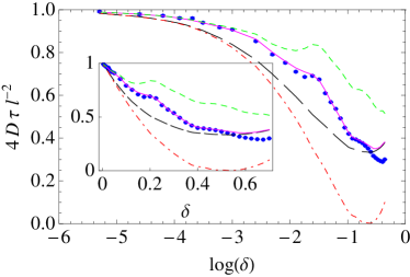
Figure 5: Numerical computation of the diffusion coefficient of the billiard table on a square lattice as shown in Fig. 4, here divided by the dimensional factor, Eq. (3). The lines correspond to the different approximate results discussed above: (long-dashed, black line) single-step memory approximation (14); (dot-dashed, red line) first-order truncation (15); (solid, magenta line) two-step memory approximation, obtained from Eqs. (4) and (37); (dashed, green line) second-order truncation (39).

The other main observation is that the truncated estimates (15) and (39) are inaccurate as soon as $\delta\gtrsim 0.05$. The reason can be traced to the anisotropy of the hopping processes. Figure 6 shows the transition rates of the single-step memory random walk. Although the probability of a right or left turn remains close to $1/4$ throughout the parameter range, the backscattering probability starts growing linearly above $1/4$ with small $\delta$’s and saturates near $1/2$ at around $\delta=0.5$. Correspondingly, the forward-scattering probability decreases and is close to zero at around $\delta=0.5$.

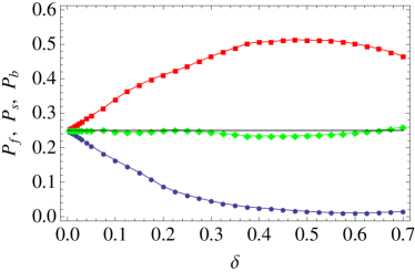
Figure 6: (Color online) Numerical computation of the transition probabilities $P_{\mathrm{b}}$ (squares), $P_{\mathrm{f}}$ (circles) and $P_{\mathrm{s}}$ (diamonds) of the single-step memory approximation associated to the billiard table on a square lattice. These rates reflect the anisotropy of the process.

Looking at the transition probabilities of the two-step memory process, shown in Fig. 7, we notice the differences among these probabilities, for instance comparing $P_{\mathrm{bb}}$, $P_{\mathrm{fb}}$ and $P_{\mathrm{sb}}$, as well as between these probabilities and that of the single-step memory process, in our example $P_{\mathrm{b}}$. These differences justify the necessity of resorting to the two-step memory process over the single-step process.

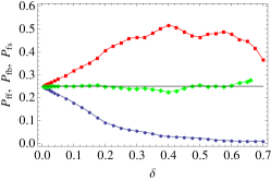
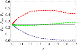
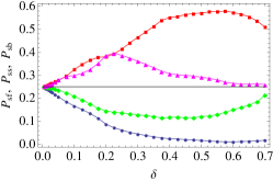
Figure 7: (Color online) Numerical computation of the transition probabilities $P_{\mathrm{xb}}$ (squares), $P_{\mathrm{xf}}$ (circles) and $P_{\mathrm{xs}}$ (diamonds) of the two-step memory approximation associated to the billiard table on a square lattice, where x stands respectively for f (left), b (middle) and s (right). In the right figure, the triangles are the probabilities of turning right after turning left and, the other way around, turning left after turning right. The differences between these three figures and the single-step transition probabilities shown in Fig. 6 justify resorting to a two-step memory process.

IV Conclusions

The diffusion coefficients of deterministic systems with rapid decay of correlations can be well approximated by that of correlated walks, where a walker’s transition probabilities are determined according to its motion over the last few steps.

Billiards provide good, physically motivated, examples of such systems. The Machta-Zwanzig dimensional prediction MZ83 , according to which the diffusion coefficient is approximated by the ratio between the distance between traps squared and the trapping time, provides a gross estimate of this quantity. However, the importance of memory effects in the deterministic diffusion of tracer particles is apparent as soon as one moves away from the limit where the trapping times are infinite.

Truncation schemes based on the Green-Kubo formula, such as considered in Kla07 ; KK02 , may provide accurate results for models with little anisotropy, but they are physically inconsistent: given a hopping process with finite memory effects, velocity auto-correlations of all orders yield non-vanishing contributions to the Green-Kubo formula.

This is particularly clear where anisotropies come into play. Estimates of the diffusion coefficients based on persistent random walks, however, do provide accurate results where the truncation schemes breakdown.

It will be interesting to find out how these results transpose to models where disorder is present, such as with tagged-particle diffusion in interacting particle systems. Dimensional predictions similar to the Machta-Zwanzig one also appeared recently in the context of models of heat conduction GG08 ; GL08 . Estimating the deviations of the heat conductivities of these models from dimensional predictions remains an open problem.

- (1) S. Chandrasekar, Stochastic problems in physics and astronomy Rev. Mod. Phys. 15, 1(1943).
- (2) P. Gaspard, Chaos, Scattering and Statistical Mechanics (Cambridge University Press, Cambridge, UK, 1998).
- (3) J. R. Dorfman, An Introduction to Chaos in Nonequilibrium Statistical Mechanics (Cambridge University Press, Cambridge, UK, 1999).
- (4) R. Klages, Microscopic chaos, fractals and transport in nonequilibrium statistical mechanics (World Scientific, Singapore, 2007).
- (5) L. A. Bunimovich and Ya. Sinai, Markov Partition for Dispersed Billiard Comm. Math. Phys. 78, 247 (1980). Statistical properties of Lorentz gas with periodic configuration of scatterers Comm. Math. Phys. 78, 479 (1980).
- (6) J. Machta and R Zwanzig, Diffusion in a periodic Lorentz gas Phys. Rev. Lett. 50 1959 (1983).
- (7) R. Klages and C. Dellago, Density-dependent diffusion in the periodic Lorentz gas J. Stat. Phys. 101 145 (2000).
- (8) R. Klages and N. Korabel, Understanding deterministic diffusion by correlated random walks J. Phys A math. gen. 35 4823 (2002).
- (9) N. Chernov and R. Markarian, Chaotic billiards Math. Surveys and Monographs 127 (AMS, Providence, RI, 2006).
- (10) R. Zwanzig, From classical dynamics to continuous time random walks J. Stat. Phys. 30 255 (1983).
- (11) B. D. Hughes, Random Walks and Random Environments. Volume 1: Random Walks (Clarendon Press, Oxford, 1995)
- (12) G. H. Weiss and R. J. Rubin Random Walks: Theory and Selected Applications Advances in Chemical Physics 52 563 (1983)
- (13) J. W. Haus and K.W. Kehr, Diffusion in regular and disordered lattices Phys. Rep. 150, 263 (1987).
- (14) G. H. Weiss, Aspects and Applications of the Random Walk (North-Holland, Amsterdam, 1994).
- (15) T. Gilbert and D. P. Sanders, Diffusion coefficients for multi-step persistent random walks on lattices unpublished.
- (16) P. Gaspard and T. Gilbert, Heat conduction and Fourier’s law by consecutive local mixing and thermalization Phys. Rev. Lett. 101 020601 (2008).
- (17) T. Gilbert and R. Lefevere, Heat Conductivity from Molecular Chaos Hypothesis in Locally Confined Billiard Systems Phys. Rev. Lett. 101 200601 (2008).