Target prediction and a statistical sampling algorithm for RNA-RNA interaction

Abstract

It has been proven that the accessibility of the target sites has a critical influence for miRNA and siRNA. In this paper, we present a program, rip2.0, not only the energetically most favorable targets site based on the hybrid-probability, but also a statistical sampling structure to illustrate the statistical characterization and representation of the Boltzmann ensemble of RNA-RNA interaction structures. The outputs are retrieved via backtracing an improved dynamic programming solution for the partition function based on the approach of Huang et al. (Bioinformatics). The $O(N^{6})$ time and $O(N^{4})$ space algorithm is implemented in C (available from http://www.combinatorics.cn/cbpc/rip2.html).

1 Introduction

Noncoding RNAs have been found to have roles in a great variety of processes, including transcriptional regulation, chromosome replication, RNA processing and modiTcation, messenger RNA stability and translation, and even protein degradation and translocation. Direct base-pairing with target RNA or DNA molecules is central to the function of some ncRNAs (Storz, 2002). Examples include the regulation of translation in both prokaryotes (Narberhaus and Vogel, 2007) and eukaryotes (McManus and Sharp, 2002; Banerjee and Slack, 2002), the targeting of chemical modifications (Bachellerie et al., 2002), as well as insertion editing (Benne, 1992), transcriptional control (Kugel and Goodrich, 2007). The common theme in many RNA classes, including miRNAs, siRNAs, snRNAs, gRNAs, and snoRNAs is the formation of RNA-RNA interaction structures that are more complex than simple sense-antisense interactions.

The hybridization energy is a widely used criterion to predict RNA-RNA interactions (Rehmsmeier et al., 2004; Tjaden et al., 2006; Busch et al., 2008). It has been proven that the accessibility of the target sites has a critical influence for miRNA and siRNA (Ameres and Schroeder, 2007; Kertesz et al., 2007; Kretschmer-Kazemi Far and Sczakiel, 2003). Although a lot regulatory ncRNAs has already been identified, the number of experimentally verified target sites is much smaller, which stimulate a great demand to restrain the list of putative targets. In its most general form, the RNA-RNA interaction problem (RIP) is NP-complete (Alkan et al., 2006; Mneimneh, 2007). The argument for this statement is based on an extension of the work of Akutsu (2000) for RNA folding with pseudoknots. Polynomial-time algorithms can be derived, however, by restricting the space of allowed configurations in ways that are similar to pseudoknot folding algorithms (Rivas and Eddy, 1999). The second major problem concerns the energy parameters since the standard loop types (hairpins, internal and multiloops) are insufficient; for the additional types, such as kissing hairpins, experimental data are virtually absent. Tertiary interactions, furthermore, are likely to have a significant impact.

Several circumscribed approaches of target prediction have been considered in the literature. The simplest approach concatenates the two interacting sequences and subsequently employs a slightly modified standard secondary structure folding algorithm. For instance, the algorithms RNAcofold (Hofacker et al., 1994; Bernhart et al., 2006), pairfold (Andronescu et al., 2005), and NUPACK (Ren et al., 2005) subscribe to this strategy. The main problem of this approach is that it cannot predict important motifs such as kissing-hairpin loops. The paradigm of concatenation has also been generalized to the pseudoknot folding algorithm of Rivas and Eddy (1999). The resulting model, however, still does not generate all relevant interaction structures (Chitsaz et al., 2009; Qin and Reidys, 2008). An alternative line of thought is to neglect all internal base-pairings in either strand and to compute the minimum free energy (mfe) secondary structure for their hybridization under this constraint. For instance, RNAduplex and RNAhybrid (Rehmsmeier et al., 2004) follows this line of thought. RNAup (Mückstein et al., 2006, 2008) and intaRNA (Busch et al., 2008) restrict interactions to a single interval that remains unpaired in the secondary structure for each partner. Due to the highly conserved interaction motif, snoRNA/target complexes are treated more efficiently using a specialized tool (Tafer et al., 2009) however. Pervouchine (2004) and Alkan et al. (2006) independently derived and implemented minimum free energy (mfe) folding algorithms for predicting the joint secondary structure of two interacting RNA molecules with polynomial time complexity. In their model, a “joint structure” means that the intramolecular structures of each molecule are pseudoknot-free, the intermolecular binding pairs are noncrossing and there exist no so-called “zig-zags”. The optimal “joint structure” can be computed in $O(N^{6})$ time and $O(N^{4})$ space by means of dynamic programming.

Recently, Chitsaz et al. (2009) and Huang et al. (2009) independently presented piRNA and rip1.0, tools that use dynamic programming algorithm to compute the partition function of “joint structures”, both in $O(N^{6})$ time. Albeit differing in design details, they are equivalent. In addition, Huang et al. (2009) identified in rip1.0 a basic data structure that forms the basis for computing additional important quantities such as the base pairing probability matrix. However, since the probabilities of hybrid is not simply a sum of the probabilities of the exterior arcs which are not independent, rip1.0 can not solve the probability of a hybrid.

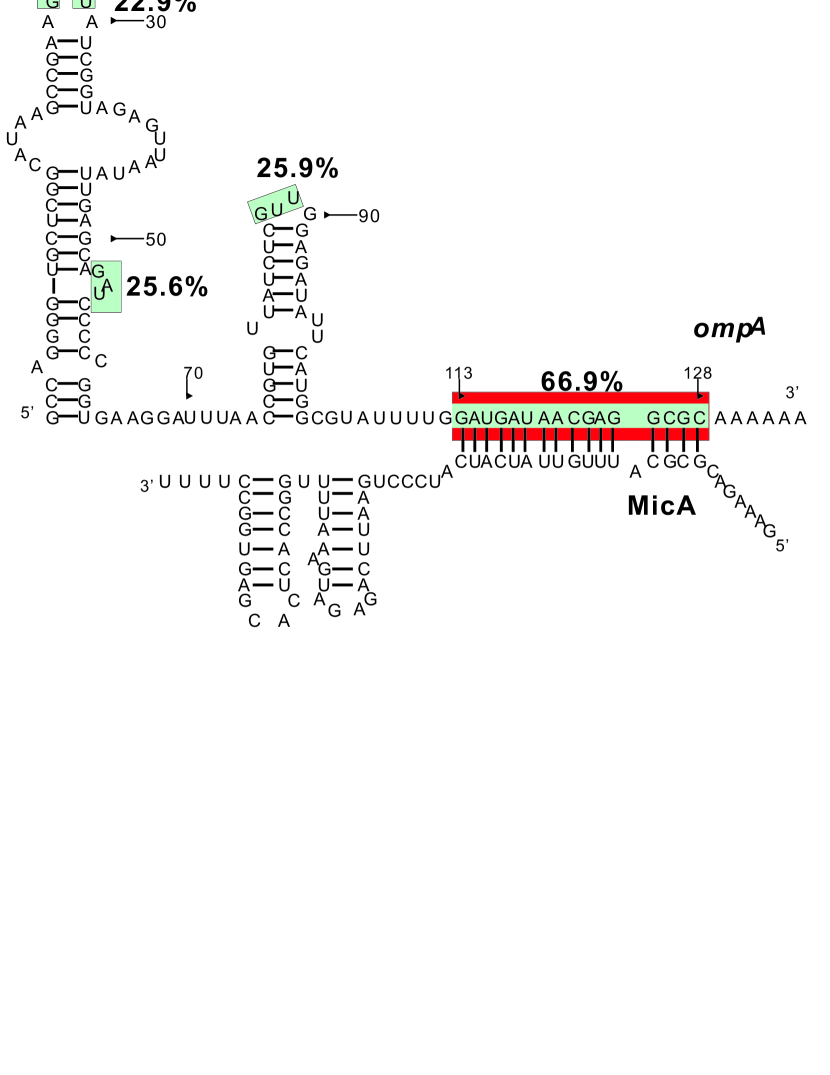
Figure 1: The natural structure of ompA-MicA (Udekwu et al., 2005), in which the target site are colored in red and the regions colored in green are the ones with the first five region-probabilities. The target sites $R[i,j]$ of $ompA$ (interacts with $MicA$) whose probabilities larger than $10^{-1}$ are showed in Tab. 1.

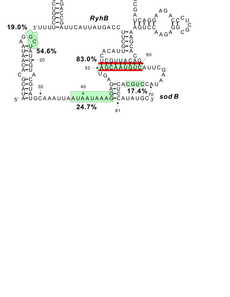
Figure 2: The natural structure of sodB-RyhB (Geissmann and Touati, 2004), in which the target site are colored in red and the regions colored in green are the ones with the first five region-probabilities. The target sites $R[i,j]$ of sodB (interacts with RyhB) whose probabilities larger than $10^{-1}$ are showed in Tab. 2.

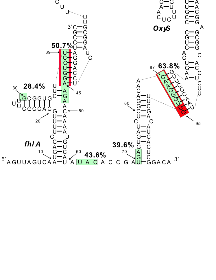
Figure 3: The natural structure of fhlA-OxyS (Chitsaz et al., 2009), in which the target site are colored in red and the regions colored in green are the ones with the first five region-probabilities. The target sites $R[i,j]$ of fhlA (interacts with OxyS) whose probabilities larger than $10^{-1}$ are showed in Tab. 3.

The calculation of equilibrium partition functions and base-pairing probabilities is an important advance toward the characterization of the Boltzmann ensemble of RNA-RNA interaction structures. However, this elegant algorithm does not generate any structures. However, as Ding and Lawrence (2003) suggested with prototype algorithms, the generation of a statistically representative sample of secondary structures may provide a resolution to this dilemma.

In contrast to rip1.0, given two RNA sequences, the output of rip2.0 consists of not only the partition function, the base pairing probability matrix, but also the contact-region probability matrix based on the hybrid probabilities via introducing a new component “hybrid” in the decomposition process and a statistically sampled RNA-RNA structure based on the probability-matrices. At the same time, we decrease the storage space from 4D-matrices and 2D-matrices to 4D-matrices and 2D-matrices.

2 Partition function

2.1 Background

Let us first review some basic concepts has been introduced by Huang et al. (2009), see supplement material (SM) for a full-version.

Given two RNA sequences $R$ and $S$ (e.g. an antisense RNA and its target) with $N$ and $M$ vertices, we index the vertices such that $R_{1}$ is the $5^{\prime}$ end of $R$ and $S_{1}$ denotes the $3^{\prime}$ end of $S$. The edges of $R$ and $S$ represent the intramolecular base pairs. A joint structure, $J(R,S,I)$, is a graph with the following properties, see Fig. 4, (B):

1. $R$, $S$ are secondary structures (each nucleotide being paired with at most one other nucleotide via hydrogen bonds, without internal pseudoknots);

2. $I$ is a set of arcs of the form $R_{i}S_{j}$ without pseudoknots, i.e., if $R_{i_{1}}S_{j_{1}}$, $R_{i_{2}}S_{j_{2}}\in I$ where $i_{1}<i_{2}$, then $j_{1}<j_{2}$ holds;

3. There are no zig-zags , see Fig. 4, (A).

Joint structures are exactly the configurations that are considered in the maximum matching approach of Pervouchine (2004), in the energy minimization algorithm of Alkan et al. (2006), and in the partition function approach of Chitsaz et al. (2009). The subgraph of a joint structure $J(R,S,I)$ induced by a pair of subsequences $\{R_{i},R_{i+1},\dots,R_{j}\}$ and $\{S_{h},S_{h+1},\dots,S_{\ell}\}$ is denoted by $J_{i,j;h,\ell}$. In particular, $J(R,S,I)=J_{1,N;1,M}$. We say $R_{a}R_{b}(S_{a}S_{b},R_{a}S_{b})\in J_{i,j;h,\ell}$ if and only if $R_{a}R_{b}(S_{a}S_{b},R_{a}S_{b})$ is an edge of the graph $J_{i,j;h,\ell}$. Furthermore, $J_{i,j;h,\ell}\subset J_{a,b;c,d}$ if and only if $J_{i,j;h,\ell}$ is a subgraph of $J_{a,b;c,d}$ induced by $\{R_{i},\dots,R_{j}\}$ and $\{S_{h},\dots,S_{\ell}\}$.

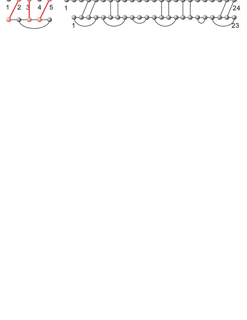
Figure 4: (A): A zigzag, generated by $R_{2}S_{1}$, $R_{3}S_{3}$ and $R_{5}S_{4}$ (red). (B): the joint structure $J_{1,24;1,23}$, we color the different segments and tight structures in which $J_{1,24;1,23}$ decomposes.

Given a joint structure, $J_{a,b;c,d}$, its tight structure (ts) $J_{a^{\prime},b^{\prime};c^{\prime},d^{\prime}}$ is either a single exterior arc $R_{a^{\prime}}S_{c^{\prime}}$ (in the case $a^{\prime}=b^{\prime}$ and $c^{\prime}=d^{\prime}$), or the minimal block centered around the leftmost and rightmost exterior arcs $\alpha_{l},\alpha_{r}$, (possibly being equal) and an interior arc subsuming both, i.e., $J_{a^{\prime},b^{\prime};c^{\prime},d^{\prime}}$ is tight in $J_{a,b;c,d}$ if it has either an arc $R_{a^{\prime}}R_{b^{\prime}}$ or $S_{c^{\prime}}S_{d^{\prime}}$ if $a^{\prime}\neq b^{\prime}$ or $c^{\prime}\neq d^{\prime}$.

In the following, a ts is denoted by $J^{T}_{i,j;h,\ell}$. If $J_{a^{\prime},b^{\prime};c^{\prime},d^{\prime}}$ is tight in $J_{a,b;c,d}$, then we call $J_{a,b;c,d}$ its envelope. By construction, the notion of ts is depending on its envelope. There are only four basic types of ts, see Fig. 5:

• $\{R_{i}S_{h}\}=J^{\circ}_{i,j;h,\ell}$ and $i=j$, $h=\ell$;

• $R_{i}R_{j}\in J^{\bigtriangledown}_{i,j;h,\ell}$ and $S_{h}S_{\ell}\not\in J^{\bigtriangledown}_{i,j;h,\ell}$;

• $\{R_{i}R_{j},S_{h}S_{\ell}\}\in J^{\square}_{i,j;h,\ell}$;

• $S_{h}S_{\ell}\in J^{\bigtriangleup}_{i,j;h,\ell}$ and $R_{i}R_{j}\not\in J^{\bigtriangleup}_{i,j;h,\ell}$.

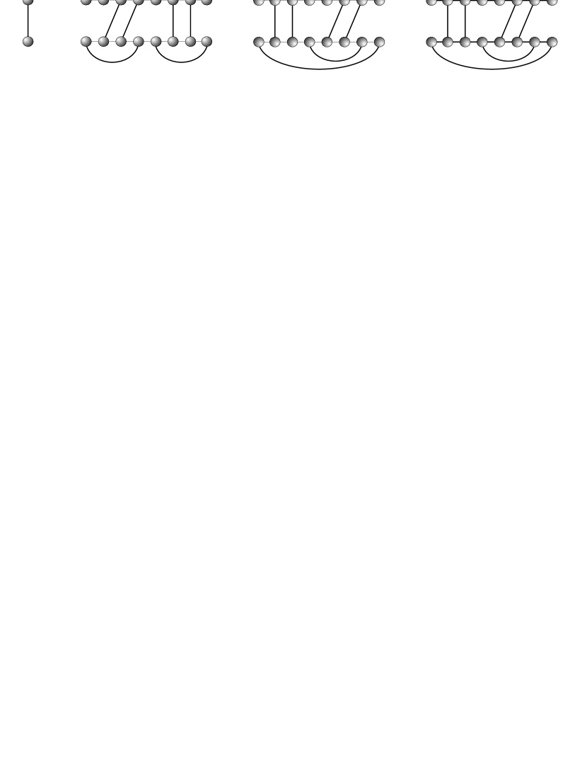
Figure 5: From left to right: tights of type $\circ$, $\bigtriangledown$, $\square$ and $\bigtriangleup$.

2.2 Refined decomposition grammar for target prediction

The unique ts decomposition would in principle already suffice to construct a partition function algorithm. Indeed, each decomposition step corresponds to a multiplicative recursion relation for the partition functions associated with the joint structures. From a practical point of view, however, this would result in an unwieldy expensive implementation. The reason are the multiple break points $a$, $b$, $c$, $d$, …, each of which correspond to a nested for-loop.

We therefore need a refined decomposition that reduced the number of break points. To this end we call a joint structure right-tight (rts), $J^{RT}_{i,j;r,s}$ in $J_{i_{1},j_{1};r_{1},s_{1}}$ if its rightmost block is a $J_{i_{1},j_{1};r_{1},s_{1}}$-ts and double-tight (dts), $J^{DT}_{i,j;r,s}$ in $J_{i_{1},j_{1};r_{1},s_{1}}$ if both of its left- and rightmost blocks are $J_{i_{1},j_{1};r_{1},s_{1}}$-ts’s. In particular, for the convenient of the computation, we assume the single interaction arc as a special case of dts, i.e. $J^{DT}_{i_{1},i_{1};r_{1},r_{1}}=R_{i_{1}}S_{r_{1}}$ . In order to obtain the probability of a hybrid $J^{\sf Hy}_{i_{1},i_{\ell};j_{1},j_{\ell}}$ via the backtracing method used in (Huang et al., 2009), we introduce the hybrid structure, $J^{\sf Hy}_{i_{1},i_{\ell};j_{1},j_{\ell}}$, as a new block item used in the decomposition process. We adopt the point of view of Algebraic Dynamic Programming (Giegerich and Meyer, 2002) and regard each decomposition rule as a production in a suitable grammar. Fig. 6 summarizes three major steps in the decomposition: (I) “interior arc-removal” to reduce ts. The scheme is complemented by the usual loop decomposition of secondary structures, and (II) “block-decomposition” to split a joint structure into two blocks.

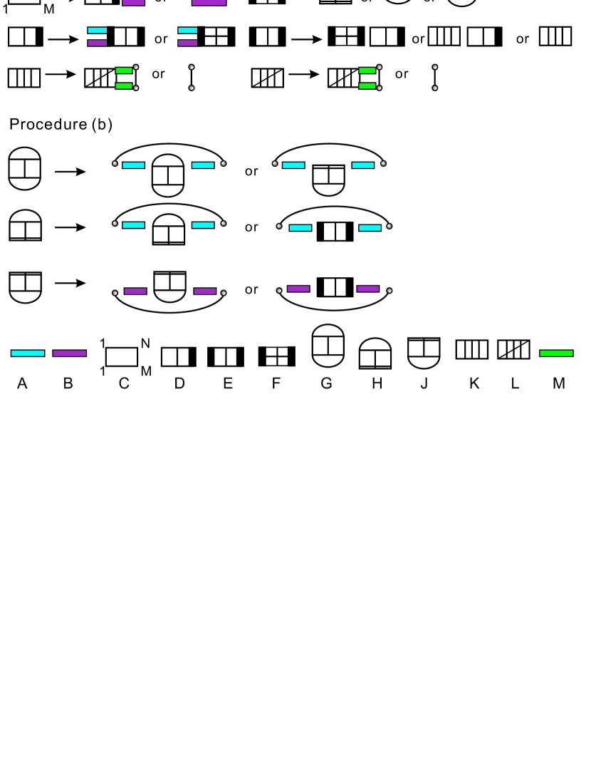
Figure 6: Illustration of Procedure (a) the reduction of arbitrary joint structures and right-tight structures, and Procedure (b) the decomposition of tight structures. The panel below indicates the 10 different types of structural components: A, B: maximal secondary structure segments $R[i,j]$, $S[r,s]$; C: arbitrary joint structure $J_{1,N;1,M}$; D: right-tight structures $J^{RT}_{i,j;r,s}$; E: double-tight structure $J^{DT}_{i,j;r,s}$; F tight structure of type $\bigtriangledown$, $\bigtriangleup$ or $\square$; G: type $\square$ tight structure $J^{\square}_{i,j;r,s}$; H: type $\bigtriangledown$ tight structure $J^{\bigtriangledown}_{i,j;r,s}$; J: type $\bigtriangleup$ tight structure $J^{\bigtriangleup}_{i,j;r,s}$; K: hybrid structure $J^{\sf Hy}_{i,j;h,\ell}$; L: substructure of a hybrid $J^{\sf h}_{i,j;h,\ell}$ such that $R_{i}S_{\ell}$ and $R_{h}S_{\ell}$ are exterior arcs; M: isolated segment $R[i,j]$ or $S[h,\ell]$.

According to the decomposition rule, a given joint structure decomposed into interior arcs and hybrids, see Figure 7 (A). The details of the decomposition procedures are collected in SM, Section 2, where we show that for each joint structure $J_{1,N;1,M}$ we indeed obtain a unique decomposition-tree (parse-tree), denoted by $T_{J_{1,N;1,M}}$. More precisely, $T_{J_{1,N;1,M}}$ has root $J_{1,N;1,M}$ and all other vertices correspond to a specific substructure of $J_{1,N;1,M}$ obtained by the successive application of the decomposition steps of Fig. 6 and the loop decomposition of the secondary structures. The decomposition trees of a concrete example generated according to rip2.0 and rip1.0 is shown in Fig. 7 (A) and (B), respectively.

Figure 7: The decomposition trees $T_{J_{1,15;1,8}}$ for the joint structure $J_{1,15;1,8}$ according to the grammar in rip2.0 (A) and rip1.0 (B), respectively.

Let us now have a closer look at the energy evaluation of $J_{i,j;h,\ell}$. Each decomposition step in Fig. 6 results in substructures whose energies we assume to contribute additively and generalized loops that need to be evaluated directly. There are the following two scenarios:

I. Interior Arc removal. The first type of decomposition is focus on decomposing ts which is similar as the approach deduced by Huang et al. (2009). Most of the decomposition operations in Procedure (b) displayed in Fig. 6 can be viewed as the “removal” of an arc (corresponding to the closing pair of a loop in secondary structure folding) followed by a decomposition. Both: the loop-type and the subsequent possible decomposition steps depend on the newly exposed structural elements. W.l.o.g., we may assume that we open an interior base pair $R_{i}R_{j}$.

For instance, a rts $J^{RT}_{p,q,r,s}$ (denoted by “D” in Fig. 6) we need to determine the type of the exposed pairs of both $R[p,q]$ and $S[r,s]$. Hence each such structure will be indexed by two types lies in $\{{\sf E},{\sf M},{\sf K},{\sf F}\}$. Analogously, there are in total four types of a hybrid $J^{\sf Hy}_{i,j;h,\ell}$, i.e.  $\{J^{\sf Hy,EE}_{i,j;h,\ell},J^{\sf Hy,EK}_{i,j;h,\ell},J^{\sf Hy,KE}_{i,j;h,\ell},J^{\sf Hy,KK}_{i,j;h,\ell}\}$.

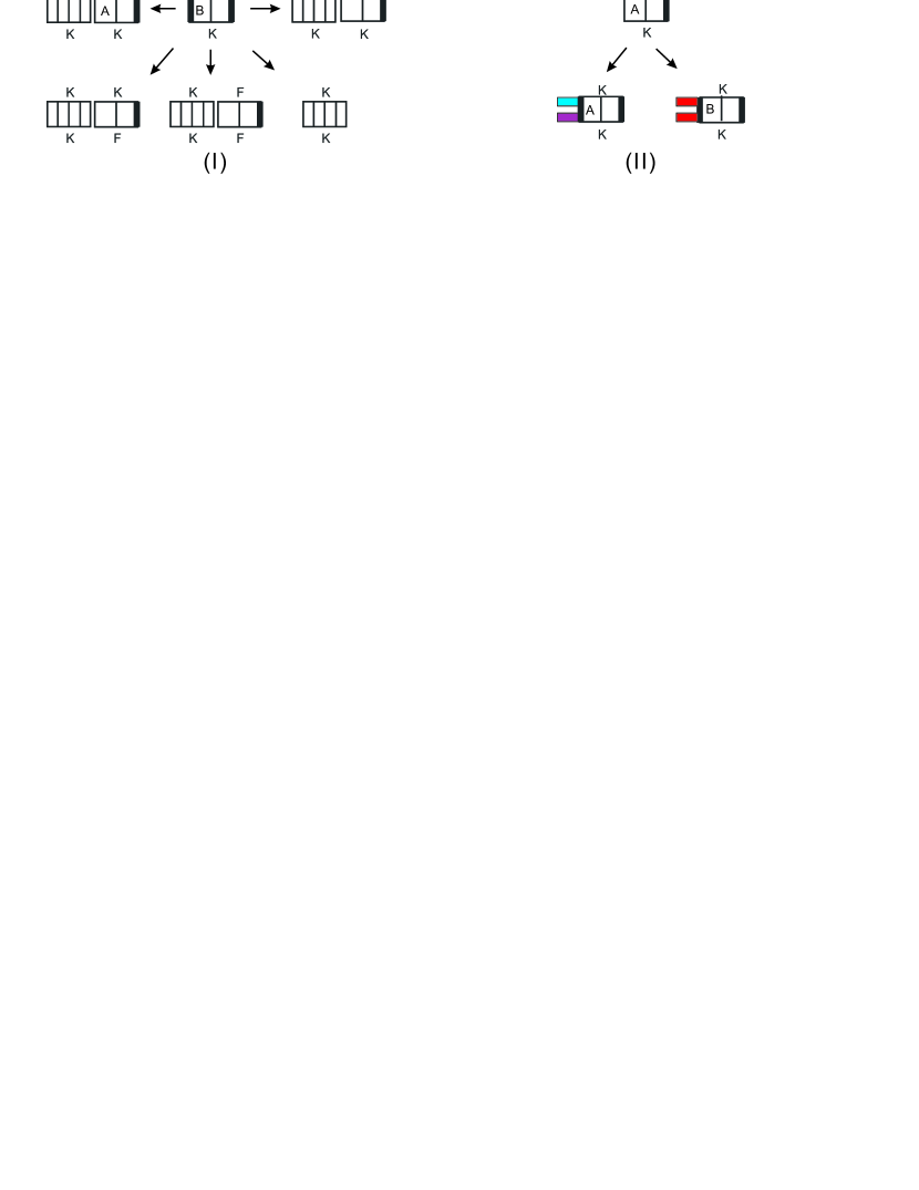
Figure 8: (I) Decomposition of $J^{RT,{\sf MK}}_{i,j;h,\ell}$ and (II) decomposition of $J^{DT,{\sf KKB}}_{i,j;h,\ell}$.

II. Block decomposition.The second type of decomposition is the splitting of joint structures into “blocks”. There are two major differences in contrast to the method used in Huang et al. (2009). First, we introduce the hybrid itself as a new block item in the grammar and furthermore decompose a hybrid via simultaneously removing a single exterior arc. Second, we split the whole interaction structure into blocks via the alternating decompositions of a rts and a dts as showed in the Procedure (a) of Fig. 6.

In order to make sure the maximality of a hybrid, the rts’s $J^{RT,KK}_{i,j;h,\ell}$, $J^{RT,KE}_{i,j;h,\ell}$, $J^{RT,EK}_{i,j;h,\ell}$ and $J^{RT,EE}_{i,j;h,\ell}$ may appear in two ways, depending on whether or not there exists an exterior arc $R_{i_{1}}S_{j_{1}}$ such that $R[i,i_{1}-1]$ and $S[j,j_{1}-1]$ are isolated segments. If there exists, we say rts is of type (B) or (A), otherwise. Similarly, a dts, $J^{RT,KK}_{i,j;h,\ell}$, $J^{RT,KE}_{i,j;h,\ell}$, $J^{RT,EK}_{i,j;h,\ell}$ or $J^{RT,EE}_{i,j;h,\ell}$ is of type (B) or (A) depending on whether $R_{i}S_{h}$ is an exterior arc. For instance, Fig. 8 (I) displays the decomposition of $J^{DT,{\sf KKB}}_{i,j;h,\ell}$ into hybrid and rts with type (A) and furthermore Fig. 8 (II) displays the decomposition of $J^{RT,{\sf KKA}}_{i,j;h,\ell}$.

Suppose $J^{DT}_{i,j;r,\ell}$ is a dts contained in a kissing loop, that is we have either $E^{e}_{R[i,j]}\neq\varnothing$ or $E^{e}_{S[h,\ell]}\neq\varnothing$. W.l.o.g., we may assume $E^{e}_{R[i,j]}\neq\varnothing$. Then at least one of the two “blocks” contains the exterior arc belonging to $E^{e}_{R[i,j]}$ labeled by ${\sf K}$ and ${\sf F}$, otherwise, see Fig. 8 (I).

2.3 Examples for partition function recursions

The computation of the partition function proceeds “from the inside to the outside”, see equs. (2.2). The recursions are initialized with the energies of individual external base pairs and empty secondary structures on subsequences of length up to four. In order to differentiate multi- and kissing-loop contributions, we introduce the partition functions $Q^{\sf{m}}_{i,j}$ and $Q^{\sf{k}}_{i,j}$. Here, $Q^{\sf{m}}_{i,j}$ denotes the partition function of secondary structures on $R[i,j]$ or $S[i,j]$ having at least one arc contained in a multi-loop. Similarly, $Q^{\sf{k}}_{i,j}$ denotes the partition function of secondary structures on $R[i,j]$ or $S[i,j]$ in which at least one arc is contained in a kissing loop. Let $\mathbb{J}^{\xi,Y_{1}Y_{2}Y_{3}}_{i,j;h,\ell}$ be the set of substructures $J_{i,j;h,\ell}\subset J_{1,N;1,M}$ such that $J_{i,j;h,\ell}$ appears in $T_{J_{1,N;1,M}}$ as an interaction structure of type $\xi\in\{DT,RT,\bigtriangledown,\bigtriangleup,\square,\circ\}$ with loop-subtypes $Y_{1},Y_{2}\in\{\sf{M},\sf{K},\sf{F}\}$ on the sub-intervals $R[i,j]$ and $S[h,\ell]$, $Y_{3}\in\{{\sf A},{\sf B}\}$. Let $Q^{\xi,Y_{1}Y_{2}Y_{3}}_{i,j;h,\ell}$ denote the partition function of $\mathbb{J}^{\xi,Y_{1}Y_{2}Y_{3}}_{i,j;h,\ell}$.

For instance, the recursion for $Q^{DT,{\sf KKB}}_{i,j;h,\ell}$ displayed in Figure 8 (I) is equivalent to:

$$\begin{split}&Q^{RT,{\sf MK}}_{i,j;h,\ell}=\sum_{i_{1},h_{1}}Q^{\sf Hy,KK}_{i,i_{1};h,h_{1}}Q^{RT,{\sf KKA}}_{i_{1}+1,j;h_{1}+1,\ell}+Q^{\sf Hy,KK}_{i,i_{1};h,h_{1}}Q^{RT,{\sf KF}}_{i_{1}+1,j;h_{1}+1,\ell}\\ &+Q^{\sf Hy,KK}_{i,i_{1};h,h_{1}}Q^{RT,{\sf FF}}_{i_{1}+1,j;h_{1}+1,\ell}+Q^{\sf Hy,KK}_{i,i_{1};h,h_{1}}Q^{RT,{\sf FK}}_{i_{1}+1,j;h_{1}+1,\ell}+Q^{{\sf HyKK}}_{i,j;h,\ell}.\end{split}$$ (2.1)

In which, the recursions for $J^{\sf Hy,EE}_{i,j;h,\ell},J^{\sf Hy,EK}_{i,j;h,\ell}$, $J^{\sf Hy,KE}_{i,j;h,\ell}$, and $J^{\sf Hy,KK}_{i,j;h,\ell}$ read:

$$\begin{split}Q^{\sf Hy,EE}_{i,j;h,\ell}&=\sum_{i_{1},h_{1}}Q^{\sf Hy,EE}_{i,i_{1};h,h_{1}}e^{-(\sigma_{0}+\sigma G^{\sf Int}_{i_{1},h_{1},j,\ell})};\\ Q^{\sf Hy,EK}_{i,j;h,\ell}&=\sum_{i_{1},h_{1}}Q^{\sf Hy,EK}_{i,i_{1};h,h_{1}}e^{-(\sigma_{0}+\sigma G^{\sf Int}_{i_{1},h_{1},j,\ell}+(\ell-h_{1}-1)\beta_{3})};\\ Q^{\sf Hy,KE}_{i,j;h,\ell}&=\sum_{i_{1},h_{1}}Q^{\sf Hy,KE}_{i,i_{1};h,h_{1}}e^{-(\sigma_{0}+\sigma G^{\sf Int}_{i_{1},h_{1},j,\ell}+(j-i_{1}-1)\beta_{3})};\\ Q^{\sf Hy,KK}_{i,j;h,\ell}&=\sum_{i_{1},h_{1}}Q^{\sf Hy,KK}_{i,i_{1};h,h_{1}}e^{-(\sigma_{0}+\sigma G^{\sf Int}_{i_{1},h_{1},j,\ell}+(j+\ell-i_{1}-h_{1}-2)\beta_{3})}.\end{split}$$ (2.2)

3 Backtracing

3.1 target prediction

Given two RNA sequences, our sample space is the ensemble of all the possible joint interaction structures. Let $Q^{I}$ denote the partition function which sums over all the possible joint structures. The probability measure of a given joint structure $J_{1,N;1,M}$ is given by

$$\mathbb{P}_{J_{1,N;1,M}}=\frac{Q_{J_{1,N;1,M}}}{Q^{I}}.$$ (3.1)

In contrast to the computation of the partition function “from the inside to the outside”, the computation of the substructure-probabilities are obtained “from the outside to the inside” via total probability formula (TPF). That is, the longest-range substructures are computed first. This is analogous to McCaskill’s algorithm for secondary structures (McCaskill, 1990).

Set $J=J_{1,N;1,M}$, $T=T_{J_{1,N;1,M}}$ and let $\Lambda_{J_{i,j;h,\ell}}=\{J|J_{i,j;h,\ell}\in T\}$ denote the set of all joint structures $J$ such that $J_{i,j;h,\ell}$ is a vertex in the decomposition tree $T$. Then

$$\mathbb{P}_{J_{i,j;h,\ell}}=\sum_{J\in\Lambda_{i,j;h,\ell}}\mathbb{P}_{J}.$$ (3.2)

By virtue of TPF, set $\theta_{s}$ be the possible parent-structure of $J_{i,j;h\ell}$ and $\mathbb{P}_{J_{i,j;h,\ell}|\theta_{i}}$ be the conditional probability, we have $\mathbb{P}_{J_{i,j;h,\ell}}=\sum_{s}\mathbb{P}_{J_{i,j;h,\ell}|\theta_{s}}\mathbb{P}_{\theta_{s}}$.

Let $\mathbb{P}^{\xi,Y_{1}Y_{2}Y_{3}}_{i,j;h,\ell}$ be the probability of $\mathbb{J}^{\xi,Y_{1}Y_{2}Y_{3}}_{i,j;h,\ell}$. For instance, $\mathbb{P}^{RT,{\sf M}{\sf K}{\sf A}}_{i,j;h,\ell}$ is the sum over all the probabilities of substructures $J_{i,j;h,\ell}\in T_{J_{1,N;1,M}}$ such that $J_{i,j;h,\ell}\in\mathbb{J}^{RT,{\sf M}{\sf K}{\sf A}}_{i,j;h,\ell}$, i.e. a rts of type ${\sf A}$ and $R[i,j]$, $S[h,\ell]$ are respectively enclosed by a multi-loop and kissing loop. Given a component, $\mathbb{J}^{\xi,Y_{1}Y_{2}Y_{3}}_{i,j;h,\ell}$ (showed in Figure 6), we say another component $\tilde{\mathbb{J}}^{\xi,Y_{1}Y_{2}Y_{3}}_{i,j;h,\ell}$ is its parent-component if and only if as a substructure, $\tilde{J}^{\xi,Y_{1}Y_{2}Y_{3}}_{i,j;h,\ell}$ could be a parent structure of ${J}^{\xi,Y_{1}Y_{2}Y_{3}}_{i,j;h,\ell}$ in the decomposition tree. Accordingly, we say $\mathbb{J}^{\xi,Y_{1}Y_{2}Y_{3}}_{i,j;h,\ell}$ is the child-component of $\tilde{\mathbb{J}}^{\xi,Y_{1}Y_{2}Y_{3}}_{i,j;h,\ell}$. For instance, $\mathbb{J}^{RT,KKB}_{i_{1},j_{1};h_{1},\ell_{1}}$ is one of the parent-component of $\mathbb{J}^{\sf Hy,KKB}_{i,j;h,\ell}$, see Figure. 8 (I). Set $\Theta_{s}$ be one of the possible parent-component of $\mathbb{J}^{\xi,Y_{1}Y_{2}Y_{3}}_{i,j;h,\ell}$. Accordingly, we have

$$\mathbb{P}^{\xi,Y_{1}Y_{2}Y_{3}}_{i,j;h,\ell}=\sum_{s}\mathbb{P}^{\xi,Y_{1}Y_{2}Y_{3}}_{i,j;h,\ell|\Theta_{s}}\mathbb{P}_{\Theta_{s}},$$ (3.3)

where by definition

$$\mathbb{P}^{\xi,Y_{1}Y_{2}Y_{3}}_{i,j;h,\ell}=\sum_{J_{i,j;h,\ell}\in\mathbb{J}^{\xi,Y_{1}Y_{2}Y_{3}}_{i,j;h,\ell}}\mathbb{P}_{J_{i,j;h,\ell}}.$$ (3.4)

Furthermore, in the programme, we calculate $\mathbb{P}^{\xi,Y_{1}Y_{2}Y_{3}}_{i,j;h,\ell|\Theta_{s}}\mathbb{P}_{\Theta_{s}}$ for all $s$ during the decomposition of $\Theta_{s}$. I.e. given $\mathbb{P}_{\Theta_{s}}$, we have $\mathbb{P}_{\Theta_{s}}=\sum_{i}\mathbb{P}_{\epsilon_{i}|\Theta_{s}}\mathbb{P}_{\Theta_{s}}$, where $\mathbb{P}_{\epsilon_{i}|\Theta_{s}}$ denotes the conditional probability of the event that given $\Theta_{s}$ is the parent-component, $\epsilon_{i}$ is its child-component. In particular, we have $\mathbb{P}^{\xi,Y_{1}Y_{2}Y_{3}}_{i,j;h,\ell|\Theta_{s}}=\mathbb{P}_{\epsilon_{m}|\Theta_{s}}$ for some $m$.

Since the four subclasses of $J^{\sf Hy}_{i,j;h,\ell}$, i.e. $J^{\sf Hy,EE}_{i,j;h,\ell},J^{\sf Hy,EK}_{i,j;h,\ell},J^{\sf Hy,KE}_{i,j;h,\ell}$, and $J^{\sf Hy,KK}_{i,j;h,\ell}$ are independent, we obtain

$$\mathbb{P}^{\sf Hy}_{i,j;h,\ell}=\mathbb{P}^{\sf Hy,EE}_{i,j;h,\ell}+\mathbb{P}^{\sf Hy,EK}_{i,j;h,\ell}+\mathbb{P}^{\sf Hy,KE}_{i,j;h,\ell}+\mathbb{P}^{\sf Hy,KK}_{i,j;h,\ell}.$$ (3.5)

Given a hybrid $J^{\sf Hy}_{i,j;h,\ell}$, recall the definition target sites are $R[i,j]$ and $S[h,\ell]$. The probability of a target site $R[i,j]$ is defined by

$$\mathbb{P}^{\sf tar}_{R[i,j]}=\sum_{h,\ell}\mathbb{P}^{\sf Hy}_{i,j;h,\ell}.$$ (3.6)

Analogously, we define $\mathbb{P}^{\sf tar}_{R[i,j]}$. We predict the optimal interaction region with maximal probability, i.e.

$$\mathbb{P}^{\sf opt}=\mathsf{max}_{i,j}\mathbb{P}^{\sf tar}_{R[i,j]}.$$ (3.7)

113,128: 66.9%	87,89: 25.9 %	53,55: 25.6 %	27,27: 23.6 %
29,29: 22.9%	39,40: 21.1 %	27,28: 20.9 %	67,69: 16.6 %
115,128: 16.6 %	36,41: 15.0 %	36,40: 13.0%	26,28: 12.3%
67,70: 10.9 %	55,56: 10.3 %

Table 1: The target sites $R[i,j]$ of ompA (interacts with MicA) whose probabilities larger than $10^{-1}$.

52,60: 83.0%	15,17: 54.6 %	38,47: 24.7 %	15,16: 19.0 %
72,75: 17.4%	77,78: 16.8 %	45,47: 14.2 %	71,74: 13.7 %
73,75: 12.3 %	77,81: 11.1 %	14,17: 11.0%

Table 2: The target sites $R[i,j]$ of sodB (interacts with RyhB) whose probabilities larger than $10^{-1}$.

87,93: 63.8%	39,48: 50.7 %	62,64: 43.6 %	70,72: 39.6 %
30,30: 28.4%	70,73: 27.0 %	39,45: 17.0 %	87,92: 13.5 %
40,45: 11.9 %	63,64: 11.4 %

Table 3: The target sites $R[i,j]$ of fhlA (interacts with OxyS) whose probabilities larger than $10^{-1}$.

3.2 Statistically generating interaction structure

In this section, we generalize the idea of Ding and Lawrence (2003) in order to draw a representative sample from the Boltzmann equilibrium distribution of RNA interaction structures. The section is divided into two parts. At first we illustrate the correspondence between the decomposition grammar, i.e. the recursions for partition functions and the sampling probabilities for mutually exclusive cases and secondly, we describe the sampling algorithm.

The calculation of the sampling probabilities is based on the recurrences of the partition functions since for mutually exclusive and exhaustive cases, the key observation is that sampling probability for a case is equivalent to the contribution to partition function by the case divided by the partition function. For instance, again we consider the decomposition of $J^{RT,{\sf MK}}_{i,j;h,\ell}$. Set $\mathbb{P}^{0}_{i_{1},j_{1}}$, $\mathbb{P}^{1}_{i_{1},j_{1}}$, $\mathbb{P}^{2}_{i_{1},j_{1}}$, $\mathbb{P}^{3}_{i_{1},j_{1}}$ and $\mathbb{P}^{4}_{i_{1},j_{1}}$ be the sampling probabilities for all five cases showed in Figure 8 (I) anticlockwise respectively, then we have:

$$\mathbb{P}^{0}_{i_{1},j_{1}} = Q^{\sf Hy,KK}_{i,i_{1};h,h_{1}}Q^{RT,{\sf KKA}}_{i_{1}+1,j;h_{1}+1,\ell}/Q^{RT,{\sf MK}}_{i,j;h,\ell},$$

$$\mathbb{P}^{1}_{i_{1},j_{1}} = Q^{\sf Hy,KK}_{i,i_{1};h,h_{1}}Q^{RT,{\sf KF}}_{i_{1}+1,j;h_{1}+1,\ell}/Q^{RT,{\sf MK}}_{i,j;h,\ell},$$

$$\mathbb{P}^{2}_{i_{1},j_{1}} = Q^{\sf Hy,KK}_{i,i_{1};h,h_{1}}Q^{RT,{\sf FF}}_{i_{1}+1,j;h_{1}+1,\ell}/Q^{RT,{\sf MK}}_{i,j;h,\ell},$$

$$\mathbb{P}^{3}_{i_{1},j_{1}} = Q^{\sf Hy,KK}_{i,i_{1};h,h_{1}}Q^{RT,{\sf FK}}_{i_{1}+1,j;h_{1}+1,\ell}/Q^{RT,{\sf MK}}_{i,j;h,\ell},$$

$$\mathbb{P}^{4}_{i_{1},j_{1}} = Q^{{\sf HyKK}}_{i,j;h,\ell}/Q^{RT,{\sf MK}}_{i,j;h,\ell}.$$

Since the probabilities of all mutually exclusive and exhaustive cases sum up to 1, we have $\sum_{i_{1},j_{1}}\mathbb{P}^{0}_{i_{1},j_{1}}+\mathbb{P}^{1}_{i_{1},j_{1}}+\mathbb{P}^{2}_{i_{1},j_{1}}+\mathbb{P}^{3}_{i_{1},j_{1}}+\mathbb{P}^{4}_{i_{1},j_{1}}=1$, which coincides with eqn. (2.1).

Next we give a description of the sampling algorithm, as a generalization of Ding and Lawrence (2003), we still take two stacks $A$ and $B$. Stack $A$ stores sub-joint structures and their types $\xi$ in the form of $\{(i,j;h,\ell;\xi)\}$, such as $(i,j;h,\ell;RT{\sf MK})$ represents a sub-joint structure $J^{RT,{\sf MK}}_{i,j;h,\ell}$. Stack $B$ collects interior/exterior arcs and unpaired bases that will define a sampled interaction structure once the sampling process finishes. At the beginning, $(1,N;1,M,arbitrary)$ is the only element in stack $A$. A sampled interaction structure is drawn recursively as follows: at first, start with $(1,N;1,M;arbitrary)$, sample a pair of separated secondary structures or a rts $(i,N;j,M;RT{\sf EE})$ according to their sampling probabilities. In the former case, $(1,N;sec)$ and $(1,M;sec)$ are stored in stack $A$. Otherwise, $(1,i-1;sec)$, $(1,j-1;sec)$ and $(i,N;j,M;RT{\sf EE})$ are stored in stack $A$. Secondly, given a new element in stack $A$, denoted by $\{(i,j;h,\ell;\xi)\}$, we draw a particular case from all the mutual exclusive and exhaustive cases according to the sampling probabilities and store the corresponding sub-joint structures into stack $A$, and all the interior arc, exterior arc or unpaired bases sampled in the process will be stored in stack $B$. I.e. after the completion of sampling for a “bigger” joint structure from stack $A$ and storage of “smaller” sub-joint structures derived in the former process in stack $A$, also the storage of the sampled arcs and unpaired bases of stack $B$, the element in the bottom of stack $A$ is chosen to do the subsequent sampling. The who process terminates when stack $A$ is empty and at the same time, a sampled interaction structure formed in stack $B$.

4 Results and conclusions

The complete set of recursions comprises for ts $Q^{\bigtriangleup,\bigtriangledown,\square}_{i,j;r,s}$, 15 4D-arrays respectively, for right-tight structures $Q^{RT}_{i,j;r,s}$, 20 4D-arrays, for dts $Q^{DT}_{i,j;r,s}$ and 20 4D-arrays. In addition, we need the usual matrices for the secondary structures $R$ and $S$, and the above mentioned matrices for kissing loops. The full set of recursions is compiled in the SM, Section 3.

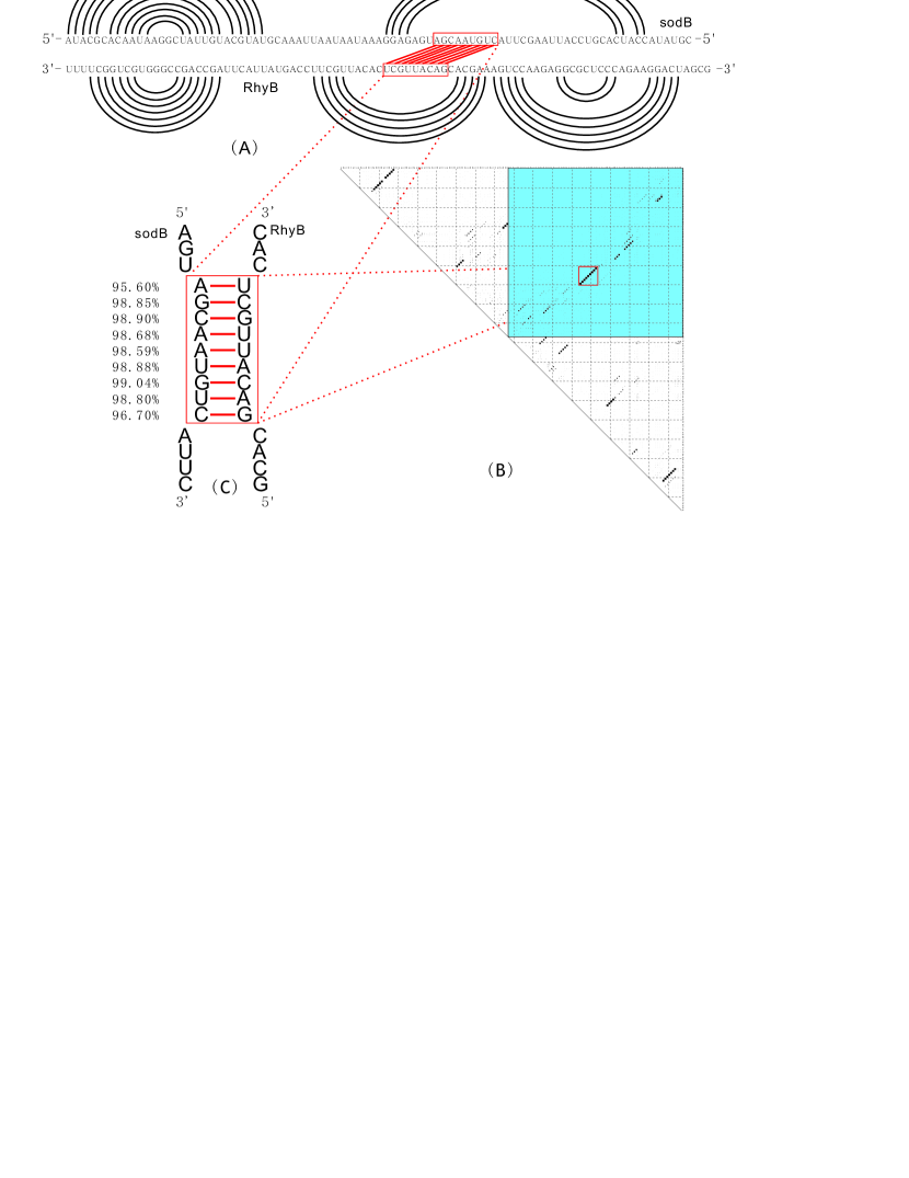
Figure 9: (A) The natural structure of sodB-RhyB (Geissmann and Touati, 2004). (B) The hybrid-probability matrix generated via rip2.0. This matrix represents all potential contact regions of the sodB structure as squares, whose area is proportional to their respective probability. (C) “Zoom” into the most likely interaction region as predicted by rip2.0. All base pairs of the hybrid are labeled by their probabilities.

Figure 10: (A) The natural structure of sodB-RhyB (Geissmann and Touati, 2004). (B) The hybrid-probability matrix generated via rip2.0. This matrix represents all potential contact regions of the sodB structure as squares, whose area is proportional to their respective probability. (C) “Zoom” into the most likely interaction region as predicted by rip2.0. All base pairs of the hybrid are labeled by their probabilities.

References

- Akutsu (2000) Akutsu, T. (2000) Dynamic programming algorithms for RNA secondary structure prediction with pseudoknots. Disc. Appl. Math., 104, 45–62.
- Alkan et al. (2006) Alkan, C., Karakoc, E., Nadeau, J., Sahinalp, S. and Zhang, K. (2006) RNA-RNA interaction prediction and antisense RNA target search. J. Comput. Biol., 13, 267–282.
- Ameres and Schroeder (2007) Ameres, S. and Schroeder, R. (2007) Molecular basis for target RNA recognition and cleavage by human RISC. Cell, 130, 101–112.
- Andronescu et al. (2005) Andronescu, M., Zhang, Z. and Condon, A. (2005) Secondary structure prediction of interacting RNA molecules. J. Mol. Biol., 345, 1101–1112.
- Bachellerie et al. (2002) Bachellerie, J., Cavaillé, J. and Hüttenhofer, A. (2002) The expanding snoRNA world. Biochimie, 84, 775–790.
- Banerjee and Slack (2002) Banerjee, D. and Slack, F. (2002) Control of developmental timing by small temporal RNAs: a paradigm for RNA-mediated regulation of gene expression. Bioessays, 24, 119–129.
- Benne (1992) Benne, R. (1992) RNA editing in trypanosomes. the use of guide RNAs. Mol. Biol.Rep., 16, 217–227.
- Bernhart et al. (2006) Bernhart, S., Tafer, H., Mückstein, U., Flamm, C., Stadler, P. and Hofacker, I. (2006) Partition function and base pairing probabilities of RNA heterodimers. Algorithms Mol. Biol., 1, 3–3.
- Busch et al. (2008) Busch, A., Richter, A. and Backofen, R. (2008) IntaRNA: efficient prediction of bacterial sRNA targets incorporating target site accessibility and seed regions. Bioinformatics, 24, 2849–2856.
- Chitsaz et al. (2009) Chitsaz, H., Salari, R., Sahinalp, S. and Backofen, R. (2009) A partition function algorithm for interacting nucleic acid strands. In press.
- Ding and Lawrence (2003) Ding, Y. and Lawrence, C. (2003) A statistical sampling algorithm for rna secondary structure prediction. Nucleic Acid Res., 31, 7280–7301.
- Geissmann and Touati (2004) Geissmann, T. and Touati, D. (2004) Hfq, a new chaperoning role: binding to messenger RNA determines access for small RNA regulator. EMBO J., 23, 396–405.
- Giegerich and Meyer (2002) Giegerich, R. and Meyer, C. (2002) Lecture Notes In Computer Science, volume 2422, chapter Algebraic Dynamic Programming, pp. 349–364. Springer-Verlag.
- Hofacker et al. (1994) Hofacker, I., Fontana, W., Stadler, P., Bonhoeffer, L., Tacker, M. and Schuster, P. (1994) Fast folding and comparison of RNA secondary structures. Monatsh. Chem., 125, 167–188.
- Huang et al. (2009) Huang, F., Qin, J., Stadler, P. and Reidys, C. (2009) Partition function and base pairing probabilities for RNA-RNA interaction prediction. Bioinformatics.
- Kertesz et al. (2007) Kertesz, M., Iovino, N., Unnerstall, U., Gaul, U. and Segal, E. (2007) The role of site accessibility in microRNA target recognition. Nat. Genet., 39, 1278–1284.
- Kretschmer-Kazemi Far and Sczakiel (2003) Kretschmer-Kazemi Far, R. and Sczakiel, G. (2003) The activity of siRNA in mammalian cells is related to strutural target accessorbility: a comparson with antisense oligonucleotides. Nucleic Acid Res., 31, 4417–4424.
- Kugel and Goodrich (2007) Kugel, J. and Goodrich, J. (2007) An RNA transcriptional regulator templates its own regulatory RNA. Nat. Struct. Mol. Biol., 3, 89–90.
- McCaskill (1990) McCaskill, J. (1990) The equilibrium partition function and base pair binding probabilities for RNA secondary structure. Biopolymers, 29, 1105–1119.
- McManus and Sharp (2002) McManus, M. and Sharp, P. (2002) Gene silencing in mammals by small interfering RNAs. Nature Reviews, 3, 737–747.
- Mneimneh (2007) Mneimneh, S. (2007) On the approximation of optimal structures for RNA-RNA interaction. IEEE/ACM Trans. Comp. Biol. Bioinf. In press, doi.ieeecomputersociety.org/10.1109/TCBB.2007.70258.
- Mückstein et al. (2008) Mückstein, U., Tafer, H., Bernhard, S., Hernandez-Rosales, M., Vogel, J., Stadler, P. and Hofacker, I. (2008) Translational control by RNA-RNA interaction: Improved computation of RNA-RNA binding thermodynamics. In Elloumi, M., Küng, J., Linial, M., Murphy, R. F., Schneider, K. and Toma, C. T. (eds.), BioInformatics Research and Development — BIRD 2008, volume 13 of Comm. Comp. Inf. Sci., pp. 114–127. Springer, Berlin.
- Mückstein et al. (2006) Mückstein, U., Tafer, H., Hackermüller, J., Bernhard, S., Stadler, P. and Hofacker, I. (2006) Thermodynamics of RNA-RNA binding. Bioinformatics, 22, 1177–1182. Earlier version in: German Conference on Bioinformatics 2005, Torda andrew and Kurtz, Stefan and Rarey, Matthias (eds.), Lecture Notes in Informatics P-71, pp 3-13, Gesellschaft f. Informatik, Bonn 2005.
- Narberhaus and Vogel (2007) Narberhaus, F. and Vogel, J. (2007) Sensory and regulatory RNAs in prokaryotes: A new german research focus. RNA Biol., 4, 160–164.
- Pervouchine (2004) Pervouchine, D. (2004) IRIS: Intermolecular RNA interaction search. Proc. Genome Informatics, 15, 92–101.
- Qin and Reidys (2008) Qin, J. and Reidys, C. (2008) A framework for RNA tertiary interaction. Submitted.
- Rehmsmeier et al. (2004) Rehmsmeier, M., Steffen, P., Höchsmann, M. and Giegerich, R. (2004) Fast and effective prediction of microRNA/target duplexes. Gene, 10, 1507–1517.
- Ren et al. (2005) Ren, J., Rastegari, B., Condon, A. and Hoos, H. (2005) Hotknots: heuristic prediction of microRNA secondary structures including pseudoknots. RNA, 11, 1494–1504.
- Rivas and Eddy (1999) Rivas, E. and Eddy, S. (1999) A dynamic programming algorithms for RNA structure prediction including pseudoknots. J. Mol. Biol., 285, 2053–2068.
- Storz (2002) Storz, G. (2002) An expanding universe of noncoding RNAs. Science, 296, 140–144.
- Tafer et al. (2009) Tafer, H., Kehr, S., Hertel, J. and Stadler, P. (2009) RNAsnoop: Efficient target prediction for box H/ACA snoRNAs. Submitted.
- Tjaden et al. (2006) Tjaden, B., Goodwin, S., Opdyke, J., Guillier, M., Fu, D., Gottesman, S. and Storz, G. (2006) Target prediction for small, noncoding RNAs in bacteria. Nucleic Acids Res., 34, 2791–2802.
- Udekwu et al. (2005) Udekwu, K., Darfeuille, F., Vogel, J., Reimegåd, J., Holmqvist, E. and Wagner, E. (2005) Hfq-dependent regulation of OmpA synthesis is mediated by an antisense RNA. Genes Dev., 19, 2355–2366.