The Infinite Hierarchical Factor Regression Model

Abstract

We propose a nonparametric Bayesian factor regression model that accounts for uncertainty in the number of factors, and the relationship between factors. To accomplish this, we propose a sparse variant of the Indian Buffet Process and couple this with a hierarchical model over factors, based on Kingman’s coalescent. We apply this model to two problems (factor analysis and factor regression) in gene-expression data analysis.

1 Introduction

Factor analysis is the task of explaining data by means of a set of latent factors. Factor regression couples this analysis with a prediction task, where the predictions are made solely on the basis of the factor representation. The latent factor representation achieves two-fold benefits: (1) discovering the latent process underlying the data; (2) simpler predictive modeling through a compact data representation. In particular, (2) is motivated by the problem of prediction in the “large P small N” paradigm [1], where the number of features $P$ greatly exceeds the number of examples $N$, potentially resulting in overfitting.

We address three fundamental shortcomings of standard factor analysis approaches [2, 3, 4, 1]: (1) we do not assume a known number of factors; (2) we do not assume factors are independent; (3) we do not assume all features are relevant to the factor analysis. Our motivation for this work stems from the task of reconstructing regulatory structure from gene-expression data. In this context, factors correspond to regulatory pathways. Our contributions thus parallel the needs of gene pathway modeling. In addition, we couple predictive modeling (for factor regression) within the factor analysis framework itself, instead of having to model it separately.

Our factor regression model is fundamentally nonparametric. In particular, we treat the gene-to-factor relationship nonparametrically by proposing a sparse variant of the Indian Buffet Process (IBP) [5], designed to account for the sparsity of relevant genes (features). We couple this IBP with a hierarchical prior over the factors. This prior explains the fact that pathways are fundamentally related: some are involved in transcription, some in signaling, some in synthesis. The nonparametric nature of our sparse IBP requires that the hierarchical prior also be nonparametric. A natural choice is Kingman’s coalescent [6], a popular distribution over infinite binary trees.

Since our motivation is an application in bioinformatics, our notation and terminology will be drawn from that area. In particular, genes are features, samples are examples, and pathways are factors. However, our model is more general. An alternative application might be to a collaborative filtering problem, in which case our genes might correspond to movies, our samples might correspond to users and our pathways might correspond to genres. In this context, all three contributions of our model still make sense: we do not know how many movie genres there are; some genres are closely related (romance to comedy versus to action); many movies may be spurious.

2 Background

Our model uses a variant of the Indian Buffet Process to model the feature-factor (i.e., gene-pathway) relationships. We further use Kingman’s coalescent to model latent pathway hierarchies.

2.1 Indian Buffet Process

The Indian Buffet Process [7] defines a distribution over infinite binary matrices, originally motivated by the need to model the latent factor structure of a given set of observations. In the standard form it is parameterized by a scale value, $\alpha$. The distribution can be explained by means of a simple culinary analogy. Customers (in our context, genes) enter an Indian restaurant and select dishes (in our context, pathways) from an infinite array of dishes. The first customer selects $Poisson(\alpha)$ dishes. Thereafter, each incoming customer $i$ selects a previously-selected dish $k$ with a probability $m_{k}/(i-1)$, where $m_{k}$ is the number of previous customers who have selected dish $k$. Customer $i$ then selects an additional $Poisson(\alpha/i)$ new dishes. We can easily define a binary matrix $\bf{Z}$ with value $Z_{ik}=1$ precisely when customer $i$ selects dish $k$. This stochastic process thus defines a distribution over infinite binary matrices.

It turn out [7] that the stochastic process defined above corresponds to an infinite limit of an exchangeable process over finite matrices with $K$ columns. This distribution takes the form $p(\textbf{Z}\textrm{~{}}\arrowvert\textrm{~{}}\alpha)=\prod_{k=1}^{K}\frac{\frac{\alpha}{K}\Gamma(m_{k}+\frac{\alpha}{K})\Gamma(P-m_{k}-1)}{\Gamma(P+1+\frac{\alpha}{K})}$, where $m_{k}=\sum_{i}Z_{ik}$ and $P$ is the total number of customers. Taking $K\rightarrow\infty$ yields the IBP. The IBP has several nice properties, the most important of which is exchangeablility. It is the exchangeablility (over samples) that makes efficient sampling algorithms possible. There also exists a two-parameter generalization to IBP where the second parameter $\beta$ controls the sharability of dishes.

2.2 Kingman’s Coalescent

Our model makes use of a latent hierarchical structure over factors; we use Kingman’s coalescent [6] as a convenient prior distribution over hierarchies. Kingman’s coalescent originated in the study of population genetics for a set of single-parent organisms. The coalescent is a nonparametric model over a countable set of organisms. It is most easily understood in terms of its finite dimensional marginal distributions over $n$ individuals, in which case it is called an $n$-coalescent. We then take the limit $n\rightarrow\infty$. In our case, the individuals are factors.

The $n$-coalescent considers a population of $n$ organisms at time $t=0$. We follow the ancestry of these individuals backward in time, where each organism has exactly one parent at time $t<0$. The $n$-coalescent is a continuous-time, partition-valued Markov process which starts with $n$ singleton clusters at time $t=0$ and evolves backward, coalescing lineages until there is only one left. We denote by $t_{i}$ the time at which the $i$th coalescent event occurs (note $t_{i}\leq 0$), and $\delta_{i}=t_{i-1}-t_{i}$ the time between events (note $\delta_{i}>0$). Under the $n$-coalescent, each pair of lineages merges indepentently with exponential rate $1$; so $\delta_{i}\sim\mathcal{E}\textit{xp}\left({n-i+1}\choose{2}\right)$. With probability one, a random draw from the $n$-coalescent is a binary tree with a single root at $t=-\infty$ and $n$ individuals at time $t=0$. We denote the tree structure by $\pi$. The marginal distribution over tree topologies is uniform and independent of coalescent times; and the model is infinitely exchangeable. We therefore consider the limit as $n\rightarrow\infty$, called the coalescent.

Once the tree structure is obtained, one can define an additional Markov process to evolve over the tree. One common choice is a Brownian diffusion process. In Brownian diffusion in $D$ dimensions, we assume an underlying diffusion covariance of $\boldsymbol{\Lambda}\in\mathbb{R}^{D\times D}$ p.s.d. The root is a $D$-dimensional vector drawn $\boldsymbol{z}$. Each non-root node in the tree is drawn Gaussian with mean equal to the value of the parent, and variance $\delta_{i}\boldsymbol{\Lambda}$, where $\delta_{i}$ is the time that has passed.

Recently, Teh et al. [8] proposed efficient bottom-up agglomerative inference algorithms for the coalescent. These (approximately) maximize the probability of $\pi$ and $\delta$s, marginalizing out internal nodes by Belief Propagation. If we associate with each node in the tree a mean $\boldsymbol{y}$ and variance $\boldsymbol{v}$ message, we update messages as Eq (1), where $i$ is the current node and $li$ and $ri$ are its children.

$$\boldsymbol{v}_{i} =\left[(\boldsymbol{v}_{{li}}+(t_{li}-t_{i})\boldsymbol{\Lambda})^{-1}+(\boldsymbol{v}_{{ri}}+(t_{ri}-t_{i})\boldsymbol{\Lambda})^{-1}\right]^{-1}$$ (1)

$$\boldsymbol{y}_{i} =\left[\boldsymbol{y}_{li}(\boldsymbol{v}_{{li}}+(t_{li}-t_{i})\boldsymbol{\Lambda})^{-1}+\boldsymbol{y}_{ri}(\boldsymbol{v}_{{ri}}+(t_{ri}-t_{i})\boldsymbol{\Lambda})^{-1}\right]^{-1}\boldsymbol{v}_{i}$$

3 Nonparametric Bayesian Factor Regression

Recall the standard factor analysis problem: $\textbf{X}=\textbf{AF}+\textbf{E}$, for standardized data X. X is a $P\times N$ matrix consisting of $N$ samples [$\boldsymbol{x}_{1},...,\boldsymbol{x}_{N}$] of $P$ features each. A is the factor loading matrix of size $P\times K$ and F = [$\boldsymbol{f}_{1},...,\boldsymbol{f}_{N}$] is the factor matrix of size $K\times N$. E = [$\boldsymbol{e}_{1},...,\boldsymbol{e}_{N}$] is the matrix of idiosyncratic variations. $K$, the number of factors, is known.

Recall that our goal is to treat the factor analysis problem nonparametrically, to model feature relevance, and to model hierarchical factors. For expository purposes, it is simplest to deal with each of these issues in turn. In our context, we begin by modeling the gene-factor relationship nonparametrically (using the IBP). Next, we propose a variant of IBP to model gene relevance. We then present the hierarchical model for inferring factor hierarchies. We conclude with a presentation of the full model and our mechanism for modifying the factor analysis problem to factor regression.

3.1 Nonparametric Gene-Factor Model

We begin by directly using the IBP to infer the number of factors. Although IBP has been applied to nonparametric factor analysis in the past [5], the standard IBP formulation places IBP prior on the factor matrix ($\bf{F}$) associating samples (i.e. a set of features) with factors. Such a model assumes that the sample-fctor relationship is sparse. However, this assumption is inappropriate in the gene-expression context where it is not the factors themselves but the associations among genes and factors (i.e., the factor loading matrix $\bf{A}$) that are sparse. In such a context, each sample depends on all the factors but each gene within a sample usually depends only on a small number of factors.

Thus, it is more appropriate to model the factor loading matrix ($\bf{A}$) with the IBP prior. Note that since A and F are related with each other via the number of factors K, modeling A nonparametrically allows our model to also have an unbounded number of factors.

For most gene-expression problems [1], a binary factor loadings matrix ($\bf{A}$) is inappropriate. Therefore, we instead use the Hadamard (element-wise) product of a binary matrix Z and a matrix V of reals. Z and V are of the same size as A. The factor analysis model, for each sample $i$, thus becomes: $\boldsymbol{x}_{i}=(\boldsymbol{Z}\odot\boldsymbol{V})\boldsymbol{f}_{i}+\boldsymbol{e}_{i}$. We have $\textbf{Z}\sim\mathcal{IBP}(\alpha,\beta)$. $\alpha$ and $\beta$ are IBP hyperparameters and have vague gamma priors on them. Our initial model assumes no factor hierarchies and hence the prior over V would simply be a Gaussian: $\textbf{V}\sim\mathcal{N}\textit{or}(0,\sigma_{v}^{2}\bf{I})$ with an inverse-gamma prior on $\sigma_{v}$. $\bf{F}$ has a zero mean, unit variance Gaussian prior, as used in standard factor analysis. Finally, $\boldsymbol{e}_{i}=\mathcal{N}\textit{or}(0,\bf{\Psi})$ models the idiosyncratic variations of genes where $\bf{\Psi}$ is a $P\times P$ diagonal matrix ($diag(\Psi_{1},...,\Psi_{P})$). Each entry $\Psi_{P}$ has an inverse-gamma prior on it.

3.2 Feature Selection Prior

Typical gene-expression datasets are of the order of several thousands of genes, most of which are not associated with any pathway (factor). In the above, these are accounted for only by the idiosyncratic noise term. A more realistic model is that certain genes simply do not participate in the factor analysis: for a culinary analogy, the genes enter the restaurant and leave before selecting any dishes. Those genes that “leave”, we term “spurious.” We add an additional prior term to account for such spurious genes; effectively leading to a sparse solution (over the rows of the IBP matrix). It is important to note that this notion of sparsity is fundamentally different from the conventional notion of sparsity in the IBP. The sparsity in IBP is over columns, not rows. To see the difference, recall that the IBP contains a “rich get richer” phenomenon: frequently selected factors are more likely to get reselected. Consider a truly spurious gene and ask whether it is likely to select any factors. If some factor $k$ is already frequently used, then a priori this gene is more likely to select it. The only downside to selecting it is the data likelihood. By setting the corresponding value in $\bf{V}$ to zero, there is no penalty.

Our sparse-IBP prior is identical to the standard IBP prior with one exception. Each customer (gene) $p$ is associated with Bernoulli random variable $T_{p}$ that indicates whether it samples any dishes. The $\bf{T}$ vector is given a parameter $\rho$, which, in turn, is given a Beta prior with parameters $a,b$.

3.3 Hierarchical Factor Model

In our basic model, each column of the matrix $\boldsymbol{Z}$ (and the corresponding column in $\boldsymbol{V}$) is associated with a factor. These factors are considered unrelated. To model the fact that factors are, in fact, related, we introduce a factor hierarchy. Kingman’s coalescent [6] is an attractive prior for integration with IBP for several reasons. It is nonparametric and describes exchangeable distributions. This means that it can model a varying number of factors. Moreover, efficient inference algorithms exist [8].

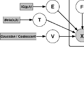
Figure 1: The graphical model for nonparametric Bayesian Factor Regression. X consists of response variables as well.

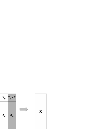
Figure 2: Training and test data are combined together and test responses are treated as missing values to be imputed

3.4 Full Model and Extension to Factor Regression

Our proposed graphical model is depicted in Figure 2. The key aspects of this model are: the IBP prior over $\bf{Z}$, the sparse binary vector $\bf{T}$, and the Coalescent prior over $\bf{V}$.

In standard Bayesian factor regression [1], factor analysis is followed by the regression task. The regression is performed only on the basis of $\bf{F}$, rather than the full data $\bf{X}$. For example, a simple linear regression problem would involve estimating a $K$-dimensional parameter vector $\boldsymbol{\theta}$ with regression value $\boldsymbol{\theta}{}^{\top}\bf{F}$. Our model, on the other hand, integrates factor regression component in the nonparametric factor analysis framework itself. We do so by prepending the responses $y_{i}$ to the expression vector $\boldsymbol{x}_{i}$ and joining the training and test data (see figure 2). The unknown responses in the test data are treated as missing variables to be iteratively imputed in our MCMC inference procedure. It is straightforward to see that it is equivalent to fitting another sparse model relating factors to responses. Our model thus allows the factor analysis to take into account the regression task as well. In case of binary responses, we add an extra probit regression step to predict binary outcomes from real-valued responses.

4 Inference

We use Gibbs sampling with a few M-H steps. The Gibbs distributions are summarized here.

Sampling the IBP matrix Z: Sampling Z consists of sampling existing dishes, proposing new dishes and accepting or rejecting them based on the acceptance ratio in the associated M-H step. For sampling existing dishes, an entry in $\bf{Z}$ is set as 1 according to $p(Z_{ik}=1|\textbf{X},Z_{-ik},\textbf{V},\textbf{F},\mathbf{\Psi})\propto\frac{m_{-i,k}}{(P+\beta-1)}p(\textbf{X}|\textbf{Z},\textbf{V},\textbf{F},\mathbf{\Psi})$ whereas it is set as 0 according to $p(Z_{ik}=0|\textbf{X},Z_{-ik},\textbf{V},\textbf{F},\mathbf{\Psi})\propto\frac{P+\beta-1-m_{-i,k}}{(P+\beta-1)}p(\textbf{X}|\textbf{Z},\textbf{V},\textbf{F},\mathbf{\Psi})$. $m_{-i,k}=\sum_{j\neq i}Z_{jk}$ is how many other customers chose dish $k$.

For sampling new dishes, we use an M-H step where we simultaneously propose $\mathbf{\eta}=(K^{new},V^{new},F^{new})$ where $K^{new}\sim Poisson(\alpha\beta/(\beta+P-1))$. We accept the proposal with an acceptance probability (following [9]) given by $a=\min\{1,\frac{p(rest|\mathbf{\eta^{*}})}{p(rest|\mathbf{\eta})}\}$. Here, $p(rest|\eta)$ is the likelihood of the data given parameters $\eta$. We propose $V^{new}$ from its prior (either Gaussian or Coalescent) but, for faster mixing, we propose $F^{new}$ from its posterior.

Sampling $V^{new}$ from the coalescent is slightly involved. As shown pictorially in figure 3, proposing a new column of $\boldsymbol{V}$ corresponds to adding a new leaf node to the existing coalescent tree. In particular, we need to find a sibling ($s$) to the new node $y^{\prime}$ and need to find an insertion point on the branch joining the sibling $s$ to its parent $p$ (the grandparent of $y^{\prime}$). Since the marginal distribution over trees under the coalescent is uniform, the sibling $s$ is chosen uniformly over nodes in the tree. We then use importance sampling to select an insertion time for the new node $y^{\prime}$ between $t_{s}$ and $t_{p}$, according to the exponential distribution given by the coalescent prior (our proposal distribution is uniform). This gives an insertion point in the tree, which corresponds to the new parent of $y^{\prime}$. We denote this new parent by $p^{\prime}$ and the time of insertion as $t$. The predictive density of the newly inserted node $y^{\prime}$ can be obtained by marginalizing the parent $p^{\prime}$. This yields $\mathcal{N}\textit{or}(\boldsymbol{y}_{0},\boldsymbol{v}_{0})$, given by:

$$\boldsymbol{v}_{0} =[(\boldsymbol{v}_{s}+(t_{s}-t)\boldsymbol{\Lambda})^{-1}+(\boldsymbol{v}_{p}+(t-t_{p})\boldsymbol{\Lambda})^{-1}]^{-1}$$

$$\boldsymbol{y}_{0} =[\boldsymbol{y}_{s}/(v_{s}+(t_{s}-t)\boldsymbol{\Lambda})+\boldsymbol{y}_{p}/(v_{p}+(t_{p}-t)\boldsymbol{\Lambda})]\boldsymbol{v}_{0}$$

Here, $y_{s}$ and $v_{s}$ are the messages passed up through the tree, while $y_{p}$ and $v_{p}$ are the messages passed down through the tree (compare to Eq (1)).

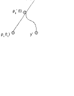
Figure 3: Adding a new node to the tree

Sampling the sparse IBP vector T: In the sparse IBP prior, recall that we have an additional $P$-many variables $T_{p}$, indicating whether gene $p$ “eats” any dishes. $T_{p}$ is drawn from Bernoulli with parameter $\rho$, which, in turn, is given a $\mathcal{B}\textit{et}(a,b)$ prior. For inference, we collapse $\rho$ and $\mathbf{\Psi}$ and get Gibbs posterior over $T_{p}$ of the form ${p(T_{p}=1|.)}\propto(a+\sum_{q\neq p}T_{p})\mathcal{S}\textit{tu}(\boldsymbol{x}_{p}|(\textbf{Z}_{p}\odot\textbf{V}_{p})\boldsymbol{F},g/h,g))$ and $p(T_{p}=0|.)\propto(b+P-\sum_{q\neq p}T_{q})\mathcal{S}\textit{tu}(\boldsymbol{x}_{p}|0,g/h,g)$, where $\mathcal{S}\textit{tu}$ is the non-standard Student’s t-distribution. $g,h$ are hyperparameters of the inverse-gamma prior on the entries of $\mathbf{\Psi}$.

Sampling the real valued matrix V: For the case when V has a Gaussian prior on it, we sample V from its posterior $p(V_{g,j}|\textbf{X},\textbf{Z},\textbf{F},\mathbf{\Psi})\propto\mathcal{N}\textit{or}(V_{g,j}|\mu_{g,j},\Sigma_{g,j})$, where $\Sigma_{g,j}=(\sum_{i=1}^{N}\frac{F_{j,i}^{2}}{\Psi_{g}}+\frac{1}{\sigma_{v}^{2}})^{-1}$ and $\mu_{g,j}=\Sigma_{g,j}(\sum_{i=1}^{N}F_{j,i}X^{*}_{g,j})\Psi_{g}^{-1}$. We define $X^{*}_{g,j}=X_{g,i}-\sum_{l=1,l\neq j}^{K}(A_{g,l}V_{g,l})F_{l,i}$, and $\textbf{A}=\textbf{Z}\odot\textbf{V}$. The hyperparameter $\sigma_{v}$ on V has an inverse-gamma prior and posterior also has the same form. For the case with coalescent prior on V, we have $\Sigma_{g,j}=(\sum_{i=1}^{N}\frac{F_{j,i}^{2}}{\Psi_{g}}+\frac{1}{{v_{0}}_{j}})^{-1}$ and $\mu_{g,j}=\Sigma_{g,j}(\sum_{i=1}^{N}F_{j,i}X^{*}_{g,j})(\Psi_{g}+\frac{{y_{0}}_{g,j}}{{v_{0}}_{j}})^{-1}$, where $\boldsymbol{y}_{0}$ and $\boldsymbol{v}_{0}$ are the Gaussian posteriors of the leaf node added in the coalescent tree (see Eq (1)), which corresponds to the column of V being sampled.

Sampling the factor matrix F: We sample for F from its posterior $p(\textbf{F}|\textbf{X},\textbf{Z},\textbf{V},\mathbf{\Psi})\propto\mathcal{N}\textit{or}(\textbf{F}|\mathbf{\mu},\mathbf{\Sigma})$ where $\bf{\mu}=\bf{A}^{T}(\bf{A}\bf{A}^{T}+\Psi)^{-1}X$ and $\bf{\Sigma}=\textbf{I}-\bf{A}^{T}(\bf{A}\bf{A}^{T}+\Psi)^{-1}\bf{A}$, where $\textbf{A}=\textbf{Z}\odot\textbf{V}$

Sampling the idiosyncratic noise term: We place an inverse-gamma prior on the diagonal entries of $\mathbf{\Psi}$ and the posterior too is inverse-gamma: $p(\Psi_{p}|.)\propto\mathcal{IG}(g+\frac{N}{2},\frac{h}{1+\frac{h}{2}tr(\textbf{E}^{T}\textbf{E})})$, where $\textbf{E}=\textbf{X}-\bf{(Z\odot V)F}$.

Sampling IBP parameters: We sample the IBP parameter $\alpha$ from its posterior: $p(\alpha|.)\sim\mathcal{G}\textit{am}(K_{+}+a,\frac{b}{1+bH_{P}(\beta)})$, where $K_{+}$ is the number of active features at any moment and $H_{P}(\beta)=\sum_{i=1}^{P}1/(\beta+i-1)$. $\beta$ is sampled from a prior proposal using an M-H step.

Sampling the Factor Tree: Use the Greedy-Rate1 algorithm [8].

5 Related Work

A number of probabilistic approaches have been proposed in the past for the problem of gene-regulatory network reconstruction [2, 3, 4, 1]. Some take into account the information on the prior network topology [2], which is not always available. Most assume the number of factors is known. To get around this, one can perform model selection via Reversible Jump MCMC [10] or evolutionary stochastic model search [11]. Unfortunately, these methods are often difficult to design and may take quite long to converge. Moreover, they are difficult to integrate with other forms of prior knowledge (eg., factor hierarchies). A somewhat similar approach to ours is the infinite independent component analysis (iICA) model of [12] which treats factor analysis as a special case of ICA. However, their model is limited to factor analysis and does not take into account feature selection, factor hierarchy and factor regression. As a generalization to the standard ICA model, [13] proposed a model in which the components can be related via a tree-structured graphical model. It, however, assumes a fixed number of components.

Structurally, our model with Gaussian-V (i.e. no hierarchy over factors) is most similar to the Bayesian Factor Regression Model (BFRM) of [1]. BFRM assumes a sparsity inducing mixture prior on the factor loading matrix A. Specifically, $A_{pk}\sim(1-\pi_{pk})\delta_{0}(A_{pk})+\pi_{pk}\mathcal{N}\textit{or}(A_{pk}|0,\tau_{k})$ where $\delta_{0}()$ is a point mass centered at zero. To complete the model specification, they define $\pi_{pk}\sim(1-\rho_{k})\delta_{0}(\pi_{pk})+\rho_{k}\mathcal{B}\textit{et}(\pi_{pk}|sr,s(1-r))$ and $\rho_{k}\sim\mathcal{B}\textit{et}(\rho_{k}|av,a(1-v))$. Now, integrating out $\pi_{pk}$ gives: $A_{pk}\sim(1-v\rho_{k})\delta_{0}(A_{pk})+v\rho_{k}\mathcal{N}\textit{or}(A_{pk}|0,\tau_{k})$. It is interesting to note that the nonparametric prior of our model (factor loading matrix defined as $\textbf{A}=\bf{Z\odot V}$) is actually equivalent to the (parametric) sparse mixture prior of the BFRM as $K\!\rightarrow\!\infty$. To see this, note that our prior on the factor loading matrix A (composed of Z having an IBP prior, and V having a Gaussian prior), can be written as $A_{pk}\sim(1-\rho_{k})\delta_{0}(A_{pk})+\rho_{k}\mathcal{N}\textit{or}(A_{pk}|0,\sigma_{v}^{2})$, if we define $\rho_{k}\sim\mathcal{B}\textit{et}(1,\alpha\beta/K)$. It is easy to see that, for BFRM where $\rho_{k}\sim\mathcal{B}\textit{et}(av,a(1-v))$, setting $a=1+\alpha\beta/K$ and $v=1-\alpha\beta/(aK)$ recovers our model in the limiting case when $K\!\rightarrow\!\infty$.

6 Experiments

In this section, we report our results on synthetic and real datasets. We compare our nonparametric approach with the evolutionary search based approach proposed in [11], which is the nonparametric extension to BFRM.

We used the gene-factor connectivity matrix of E-coli network (described in [14]) to generate a synthetic dataset having 100 samples of 50 genes and 8 underlying factors. Since we knew the ground truth for factor loadings in this case, this dataset was ideal to test for efficacy in recovering the factor loadings (binding sites and number of factors). We also experimented with a real gene-expression data which is a breast cancer dataset having 251 samples of 226 genes and 5 prominent underlying factors (we know this from domain knowledge).

6.1 Nonparametric Gene-Factor Modeling and Variable Selection

For the synthetic dataset generated by the E-coli network, the results are shown in figure 4 comparing the actual network used to generate the data and the inferred factor loading matrix. As shown in figure 4, we recovered exactly the same number (8) of factors, and almost exactly the same factor loadings (binding sites and number of factors) as the ground truth. In comparison, the evolutionary search based approach overestimated the number of factors and the inferred loadings clearly seem to be off from the actual loadings (even modulo column permutations).

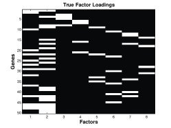
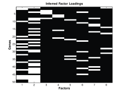
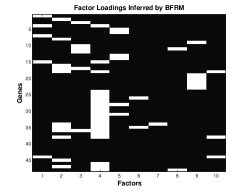
Figure 4: (Left and middle) True and inferred factor loadings (with our approach) for the synthetic data with P=50, K=8 generated using connectivity matrix of E-coli data. (Right) Inferred factor loadings with the evolutionary search based approach. White rectangles represent active sites. The data also has added noise with signal-to-noise-ratio of 10

Our results on real data are shown in figure 5. To see the effect of variable selection for this data, we also introduced spurious genes by adding 50 random features in each sample. We observe the following: (1) Without variable selection being on, spurious genes result in an overestimated number of factors and falsely discovered factor loadings for spurious genes (see figure 5), (2) Variable selection, when on, effectively filters out spurious genes, without overestimating the number of factors (see figure 5). We also investigated the effect of noise on the evolutionary search based approach and it resulted in an overestimated number of factor, plus false discovered factor loadings for spurious genes (see figure 5). To conserve space, we do not show here the cases when there are no spurious genes in the data but it turns out that variable selection does not filter out any of 226 relevant genes in such a case.

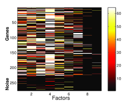
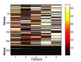
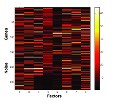
Figure 5: Effect of spurious genes (heat-plots of factor loading matrix shown): (a) Standard IBP (b) Our model with variable selection (c) The evolutionary search based approach

6.2 Hierarchical Factor Modeling

Our results with hierarchical factor modeling are shown in figure 6 for synthetic and real data. As shown, the model correctly infers the gene-factor associations, the number of factors, and the factor hierarchy. There are several ways to interpret the hierarchy. From the factor hierarchy for E-coli data (figure 6), we see that column-2 (corresponding to factor-2) of the V matrix is the most prominent one (it regulates the highest number of genes), and is closest to the tree-root, followed by column-2, which it looks most similar to. Columns corresponding to lesser prominent factors are located further down in the hierarchy (with appropriate relatedness). Figure 6 (d) can be interpreted in a similar manner for breast-cancer data. The hierarchy can be used to find factors in order of their prominence. The higher we chop off the tree along the hierarchy, the more prominent the factors, we discover, are. For instance, if we are only interested in top 2 factors in E-coli data, we can chop off the tree above the sixth coalescent point. This is akin to the agglomerative clustering sense which is usually done post-hoc. In contrast, our model discovers the factor hierarchies as part of the inference procedure itself. At the same time, there is no degradation of data reconstruction (in mean squared error sense) and the log-likelihood, when compared to the case with Gaussian prior on V (see figure 7 - they actually improve). We also show in section 6.3 that hierarchical modeling results in better predictive performance for the factor regression task. Empirical evidences also suggest that the factor hierarchy leads to faster convergence since most of the unlikely configurations will never be visited as they are constrained by the hierarchy.

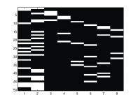
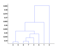
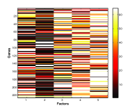
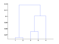
Figure 6: Hierarchical factor modeling results. (a) Factor loadings for E-coli data. (b) Inferred hierarchy for E-coli data. (c) Factor loadings for breast-cancer data. (d) Inferred hierarchy for breast-cancer data..

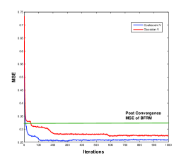
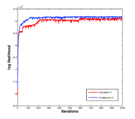
Model	Binary	Real
	(%error,std dev)	(MSE)
LogReg	17.5 (1.6)	-
BFRM	19.8 (1.4)	0.48
Nor-V	15.8 (0.56)	0.45
Coal-V	14.6 (0.48)	0.43
PredModel	18.1 (2.1)	-

Figure 7: (a) MSE on the breast-cancer data for BFRM (horizontal line), our model with Gaussian (top red curved line) and Coalescent (bottom blue curved line) priors. This MSE is the reconstruction error for the data - different from the MSE for the held-out real valued responses (fig 7 c) (b) Log-likelihoods for our model with Gaussian (bottom red curved line) and Coalescent (top blue curved line) priors. (c) Factor regression results

6.3 Factor Regression

We report factor regression results for binary and real-valued responses and compare both variants of our model (Gaussian V and Coalescent V) against 3 different approaches: logistic regression, BFRM, and fitting a separate predictive model on the discovered factors (see figure 7 (c)). The breast-cancer dataset had two binary response variables (phenotypes) associated with each sample. For this binary prediction task, we split the data into training-set of 151 samples and test-set of 100 samples. This is essentially a transduction setting as described in section 3.4 and shown in figure 2. For real-valued prediction task, we treated a 30x20 block of the data matrix as our held-out data and predicted it based on the rest of the entries in the matrix. This method of evaluation is akin to the task of image reconstruction [15]. The results are averaged over 20 random initializations and the low error variances suggest that our method is fairly robust w.r.t. initializations.

7 Conclusions and Discussion

We have presented a fully nonparametric Bayesian approach to sparse factor regression, modeling the gene-factor relationship using a sparse variant of the IBP. However, the true power of nonparametric priors is evidenced by the ease of integration of task-specific models into the framework. Both gene selection and hierarchical factor modeling are straightforward extensions in our model that do not significantly complicate the inference procedure, but lead to improved model performance and more understandable outputs. We applied Kingman’s coalescent as a hierarhical model on V, the matrix modulating the expression levels of genes in factors. An interesting open question is whether the IBP can, itself, be modeled hierarchically.

References

- [1] M. West. Bayesian Factor Regression Models in the “Large p, Small n” Paradigm. In Bayesian Statistics 7, 2003.
- [2] C. Sabatti and G. James. Bayesian Sparse Hidden Components Analysis for Transcription Regulation Networks,. Bioinformatics 22, 2005.
- [3] G. Sanguinetti, N. D. Lawrence, and M. Rattray. Probabilistic Inference of Transcription Factor Concentrations and Gene-specific Regulatory Activities. Bioinformatics, 22(22), 2006.
- [4] M. J. Beal, F. Falciani, Z. Ghahramani, C. Rangel, and D. L. Wild. A Bayesian Approach to Reconstructing Genetic Regulatory Networks with Hidden Factors. Bioinformatics, 21(3), 2005.
- [5] Z. Ghahramani, T.L. Griffiths, and P. Sollich. Bayesian Nonparametric Latent Feature Models. In Bayesian Statistics 8. Oxford University Press, 2007.
- [6] J. F. C. Kingman. The coalescent. Stochastic Processes and their Applications, 1982.
- [7] T. Griffiths and Z. Ghahramani. Infinite Latent Feature Models and the Indian Buffet Process. In Advances in Neural Information Processing Systems 18, 2006.
- [8] Y. W. Teh, H. Daumé III, and D. M. Roy. Bayesian Agglomerative Clustering with Coalescents. In Advances in Neural Information Processing Systems, volume 20, 2008.
- [9] E. Meeds, Z. Ghahramani, R. M. Neal, and S. T. Roweis. Modeling Dyadic Data with Binary Latent Factors. In Advances in Neural Information Processing Systems 19. 2007.
- [10] P. Green. Reversible jump markov chain monte carlo computation and bayesian model determination. Biometrica 82, 1995.
- [11] C. Carvalho, J. Lucas, Q. Wang, J. Chang, J. Nevins, and M. West. High-Dimensional Sparse Factor Modelling - Applications in Gene Expression Genomics. In JASA, 2008.
- [12] D. Knowles and Z. Ghahramani. Infinite Sparse Factor Analysis and Infinite Independent Components Analysis. In ICA 2007, 2007.
- [13] Francis R. Bach and Michael I. Jordan. Beyond independent components: trees and clusters. Journal of Machine Learning Research, pages 1205–1233, 2003.
- [14] I. Pournara and L. Wernisch. Factor Analysis for Gene Regulatory Networks and Transcription Factor Activity Profiles. BMC Bioinformatics, 2007.
- [15] J. J. Verbeek, S. T. Roweis, and N. Vlassis. Non-linear CCA and PCA by Alignment of Local Models. In Advances in Neural Information Processing Systems 16. 2004.