Fisher-information and the thermodynamics of scale-invariant systems

Abstract

We present a thermodynamic formulation for scale-invariant systems based on the minimization with constraints of Fisher’s information measure. In such a way a clear analogy between these systems’s thermal properties and those of gases and fluids is seen to emerge in natural fashion. We focus attention on the non-interacting scenario, speaking thus of scale-free ideal gases (SFIGs) and present some empirical evidences regarding such disparate systems as electoral results, city populations and total citations in Physics journals, that seem to indicate that SFIGs do exist. We also illustrate the way in which Zipf’s law can be understood in a thermodynamical context as the surface of a finite system. Finally, we derive an equivalent microscopic description of our systems which totally agrees with previous numerical simulations found in the literature.

1 Introduction

Scale-invariant phenomena are rather abundant in Nature and display somewhat unexpected features. Examples can be found that range from physical and biological to technological and social sciences [1]. One may cite, among many possibilities, that empirical data from percolation theory and nuclear multifragmentation [2] reflect scale-invariant behaviour, as does the abundance of genes in various organisms and tissues [3]. Additionally, we can speak of the frequency of words in natural languages [4], scientific collaboration networks [5], the Internet traffic [6], Linux packages links [7], as well as of electoral results [8, 9], urban agglomerations [10, 11] and firm sizes all over the world [12]. What characterizes these disparate systems is the lack of a characteristic size, length or frequency for an observable $k$ under scrutiny. This fact usually leads to a power law distribution $p(k)$, valid in most of the domain of definition of $k$,

$$p(k)\sim 1/k^{1+\gamma},$$ (1)

with $\gamma\geq 0$. Special attention deserves the class of universality defined by $\gamma=1$, which corresponds to the so-called Zipf’s law in the cumulative distribution or the rank-size distribution [2, 3, 4, 6, 7, 10, 11, 12, 13]. Recently, Maillart et al. [7] have found that links’ distributions follow Zipf’s law as a consequence of stochastic proportional growth. In its simplest formulation such kind of growth assumes that an element of the system becomes enlarged proportionally to its size $k$, being governed by a Wiener process. The class $\gamma=1$ emerges from the condition of stationarity, i.e., when the system reaches a dynamic equilibrium [13]. We will as well propose to consider the case $\gamma=0$ as representative of a second class of universality, since the ensuing behavior, empirically found by Costa Filho et al. [8] with regards to the vote-distribution in Brazilian electoral results, emerges as the result of multiplicative processes in complex networks [9].

In this paper we attempt to formulate a thermodynamic treatment common to these systems. Our efforts are based on the minimization with appropriate constraints of Fisher’s information measure (FIM), abbreviated as the MFI approach. It is shown in [14] that MFI leads to a (real) Schreodinger-like equation whose “potential” function is given by the constraints employed to constrain the variational process. The interplay between constraints and associated Lagrange multipliers turns our to be Legendre-invariant [14] and leads to all known thermodynamic relations. Such result constitutes the essential ingredient of our considerations here. We will first consider the MFI treatment of the ideal gas (Seccion 3), not given elsewhere as far as we are aware of, since it is indispensable to deal with it in order to fully understand the methodology employed for scale-free systems, which is tackled in Section 4. Applicatioms are discussed in Section 5 and some conclusiones drawn in Section 6. We begin our considerations in Section 2 with a brief Fisher’s sketch.

2 Minimum Fisher Information approach (MFI)

The Fisher information measure $I$ for a system described by a set of coordinates $\mathbf{q}$ and physical parameters $\mathbf{\theta}$, has the form [15]

$$I(F)=\int_{\Omega}d\mathbf{q}F(\mathbf{q}|\mathbf{\theta})\sum_{ij}c_{ij}\frac{\partial}{\partial\theta_{i}}\ln F(\mathbf{q}|\mathbf{\theta})\frac{\partial}{\partial\theta_{j}}\ln F(\mathbf{q}|\mathbf{\theta}),$$ (2)

where $F(\mathbf{q}|\mathbf{\theta})$ is the density distribution in a configuration space ($\mathbf{q}$) of volume $\Omega$ conditioned by the physical parameters collectively represented by the variable $\mathbf{\theta}$. The constants $c_{ij}$ account for dimensionality, and take the form $c_{ij}=c_{i}\delta_{ij}$ if $q_{i}$ and $q_{j}$ are uncorrelated, where $\delta_{ij}$ is the Kronecker delta. As shown in [14], the thermal-equilibrium state of the system can be determined by minimizing $I$ subject to adequate prior conditions (MFI), like the normalization of $F$ or by any constraint on the mean value of an observable $\langle A_{i}\rangle$ [14]. The MFI is then cast as a variation problem of the form

$$\delta\left\{I(F)-\sum_{i}\mu_{i}\langle A_{i}\rangle\right\}=0,$$ (3)

where $\mu_{i}$ are appropriate Lagrange multipliers.

3 MFI treatment of the ideal gas

As a didactic introductory example, not discussed in [14], we will here rederive, via MFI (something original as far as we know), the density distribution, in configuration space, of the (translational invariant) ideal gas (IG) [16], that describes non-interacting classical particles of mass $m$ with coordinates $\mathbf{q}=(\mathbf{r},\mathbf{p})$, where $md\mathbf{r}/dt=\mathbf{p}$. The translational invariance is described by the translational family of distributions $F(\mathbf{r},\mathbf{p}|\mathbf{\theta}_{r},\mathbf{\theta}_{p})=F(\mathbf{r}^{\prime},\mathbf{p}^{\prime})$ whose form does not change under the transformations $\mathbf{r}^{\prime}=\mathbf{r}-\mathbf{\theta}_{r}$ and $\mathbf{p}^{\prime}=\mathbf{p}-\mathbf{\theta}_{p}$. We assume that these coordinates are canonical [17] and uncorrelated. This assumption is introduced into the information measure (2) setting $c_{ij}=c_{i}\delta_{ij}$, where $c_{i}=c_{r}$ for space coordinates, $c_{i}=c_{p}$ for momentum coordinates. The density can obviously be factorized in the fashion $F(\mathbf{r},\mathbf{p})=\rho(\mathbf{r})\eta(\mathbf{p})$, and then [15] it follows from the additivity of the information measure that $I=I_{r}+I_{p}$. If $D$ is the dimensionality we have

$$\begin{array}[]{rl}I_{r}=&\displaystyle c_{r}\int d^{D}\mathbf{r}~{}\rho(\mathbf{r})\left|\mathbf{\nabla}_{r}\ln\rho(\mathbf{r})\right|^{2}\\ I_{p}=&\displaystyle c_{p}\int d^{D}\mathbf{p}~{}\eta(\mathbf{p})\left|\mathbf{\nabla}_{p}\ln\eta(\mathbf{p})\right|^{2}.\end{array}$$ (4)

In extremizing FIM we constrain the normalization of $\rho(\mathbf{r})$ and $\eta(\mathbf{p})$ to the total number of particles $N$ and to $1$, respectively, i.e.,

$$\int d^{D}\mathbf{r}~{}\rho(\mathbf{r})=N,\qquad\int d^{D}\mathbf{p}~{}\eta(\mathbf{p})=1.$$ (5)

In addition, we penalize infinite values for the particle momentum with a constraint on the variance of $\eta(\mathbf{p})$ to a given empirically obtained value, namely,

$$\int d^{D}\mathbf{p}~{}\eta(\mathbf{p})(\mathbf{p}-\overline{\mathbf{p}})^{2}=D\sigma_{p}^{2},$$ (6)

where $\overline{\mathbf{p}}$ is the mean value of $\mathbf{p}$. For each degree of freedom it is known from the Virial Theorem that the variance is related to the temperature $T$ as $\sigma_{p}^{2}=mk_{B}T$, with $k_{B}$ the Boltzmann constant. Variation thus yields

$$\delta\left\{c_{r}\int d^{D}\mathbf{r}~{}\rho\left|\mathbf{\nabla}_{r}\ln\rho\right|^{2}+\mu\int d^{D}\mathbf{r}~{}\rho\right\}=0$$ (7)

and

$$\delta\left\{c_{p}\int d^{D}\mathbf{p}~{}\eta\left|\mathbf{\nabla}_{p}\ln\eta\right|^{2}+\lambda\int d^{D}\mathbf{p}~{}\eta(\mathbf{p}-\overline{\mathbf{p}})^{2}+\nu\int d^{D}\mathbf{p}~{}\eta\right\}=0,$$ (8)

where $\mu$, $\lambda$ and $\nu$ are Lagrange multipliers. Introducing now $\rho(\mathbf{r})=\Psi^{2}(\mathbf{r})$ and varying (7) with respect to $\Psi$ leads to a Schroedinger-like equation [14, 18]

$$\left[-4\nabla_{r}^{2}+\mu^{\prime}\right]\Psi(\mathbf{r})=0,$$ (9)

where $\mu^{\prime}=\mu/c_{r}$. To fix the boundary conditions, we first assume that the $N$ particles are confined in a box of volume $V$, and next we take the thermodynamic limit $N,V\rightarrow\infty$ with $N/V$ finite. The equilibrium state compatible with this limit corresponds to the ground state solution ($\mu^{\prime}=0$), which is the uniform density $\rho(\mathbf{r})=N/V$.

Introducing $\eta(\mathbf{p})=\Phi^{2}(\mathbf{p})$ and varying (8) with respect to $\Phi$ leads to the quantum harmonic oscillator-like equation [18]

$$\left[-4\nabla_{p}^{2}+\lambda^{\prime}(\mathbf{p}-\overline{\mathbf{p}})^{2}+\nu^{\prime}\right]\Phi(\mathbf{p})=0,$$ (10)

where $\lambda^{\prime}=\lambda/c_{p}$ and $\nu^{\prime}=\nu/c_{p}$. The equilibrium configuration corresponds to the ground state solution, which is now a gaussian distribution. Using (6) to identify $|\lambda^{\prime}|^{-1/2}=\sigma_{p}^{2}$ we get the Maxwell-Boltzmann distribution, which leads to a density distribution in configuration space of the form

$$f(\mathbf{r},\mathbf{p})=\frac{N}{V}\frac{\exp\left[-(\mathbf{p}-\overline{\mathbf{p}})^{2}/2\sigma_{p}^{2}\right]}{(2\pi\sigma_{p}^{2})^{D/2}}.$$ (11)

If $H$ is the elementary volume in phase space, the total number of microstates is $Z=N!H^{DN}\prod_{i=1}^{N}F_{1}(\mathbf{r}_{i},\mathbf{p}_{i})$, where $F_{1}=F/N$ is the monoparticular distribution and $N!$ counts all possible permutations for distinguishable particles. The entropy $S=-k_{B}\ln Z$ gets then written in the form

$$S=Nk_{B}\left\{\ln\frac{V}{N}\left(\frac{2\pi\sigma_{p}^{2}}{H^{2}}\right)^{D/2}+\frac{2+D}{2}\right\},$$ (12)

where we have used the Stirling approximation for $N!$. This expression agrees, of course with the known value entropic expression for the IG [16], illustrating on the predictive power of the MFI formulation advanced in [14].

4 Scale invariant systems

We pass now to the leit-motif of the present communication and consider a one-dimensional system with dynamical coordinates $\mathbf{q}=(k,v)$ where $dk/d\tau=v$, with $\tau$ the time variable. We define $k$ as a discrete coordinate, i.e. $k=k_{1},k_{2},\ldots,k_{M}$, where $k_{i}=i\Delta k$ and $M\gg 1$, is the total number of bins of width $\Delta k$ in our system. In order to address the scale-invariance behaviour of $k$ we change variables passing to new coordinates $u=\ln k$ and $w=du/dt$. We work under the hypothesis that $u$ and $w$ are canonically conjugated [17] and uncorrelated. This assumption immediately leads to proportional growth since

$$dk/dt=v=kw.$$ (13)

For constant $w$ this equation yields an exponential growth $k=k_{0}e^{wt}$, which represents uniform linear motion in $u$, that is, $u=wt+u_{0}$, with $u_{0}=\ln k_{0}$ . It is easy to check that the scale transformation $k^{\prime}=k/\theta_{k}$ leaves invariant the coordinate $w$, whereas the coordinate $u$ transforms translationally as $u^{\prime}=u-\Theta_{k}$, where $\Theta_{k}=\ln\theta_{k}$. Thus, the physics does not depend on scale and the system is translationally invariant with respect to the coordinates $u$ and $w$, entailing that the distribution of physical elements can be described by the monoparametric translation families $f(u,w|\Theta_{k},\Theta_{w})=f(u^{\prime},w^{\prime})$. By analogy with the IG, we will call our system a “scale-free ideal gas” (SFIG), i.e., a system of $N$ non-interacting elements. Taking into account that i) $u$ and $w$ are canonical and uncorrelated ($c_{ii}=c_{i}\neq 0$ and $c_{uw}=c_{wu}=0$), so the density distribution can be factorized as $f(u,w)=g(u)h(w)$, and ii) that the Jacobian for our change of variables is $dkdv=e^{2u}dudw$, the information measure $I=I_{u}+I_{w}$ can be obtained in the continuous limit as

$$\begin{array}[]{rl}I_{u}=&\displaystyle c_{u}\int_{\Omega}du~{}e^{2u}g(u)\left|\frac{\partial\ln g(u)}{\partial u}\right|^{2}\\ I_{w}=&\displaystyle c_{w}\int_{-\infty}^{\infty}dw~{}h(w)\left|\frac{\partial\ln h(w)}{\partial w}\right|^{2},\end{array}$$ (14)

where $\Omega=\ln(k_{M}/k_{1})=\ln M$ is the volume defined in “$u$”-space.

4.1 MFI treatment of the scale-free ideal gas

The constraints to the given observables $\langle A_{i}\rangle$ in the extremization problem determine the behaviour of the system. For the general case, we constrain the normalization of $g(u)$ and $h(w)$ to the total number of particles $N$ and to $1$, respectively

$$\int_{\Omega}du~{}e^{2u}g(u)=N,\qquad\int_{-\infty}^{\infty}dw~{}h(w)=1.$$ (15)

In addition, we penalize infinite values for $w$ with a constraint on the variance of $h(w)$ to a given measured value

$$\int_{-\infty}^{\infty}dw~{}h(w)(w-\overline{w})^{2}=\sigma_{w}^{2},$$ (16)

where $\overline{w}$ is the average growth. The variation yields

$$\delta\left\{c_{u}\int_{\Omega}du~{}e^{2u}g\left|\frac{\partial\ln g}{\partial u}\right|^{2}+\mu\int_{\Omega}du~{}e^{2u}g\right\}=0$$ (17)

and

$$\delta\left\{c_{w}\int_{-\infty}^{\infty}dw~{}h\left|\frac{\partial\ln h}{\partial w}\right|^{2}+\lambda\int_{-\infty}^{\infty}dw~{}h(w-\overline{w})^{2}+\nu\int_{-\infty}^{\infty}dw~{}h\right\}=0,$$ (18)

where $\mu$, $\lambda$ and $\nu$ are Lagrange multipliers. Introducing $g(u)=e^{-2u}\Psi^{2}(u)$, and varying  (17) with respect to $\Psi$ leads, as is always the case with the MFI [14], to the Schroedinger-like equation

$$\left[-4\frac{\partial^{2}}{\partial u^{2}}+4+\mu^{\prime}\right]\Psi(u)=0,$$ (19)

where $\mu^{\prime}=\mu/c_{u}$. Analogously to the IG, we impose solutions compatible with a finite normalization of $g$ in the thermodynamic limit $N,\Omega\rightarrow\infty$ with $N/\Omega=\rho_{0}$ finite, where $\rho_{0}$ is defined as the bulk density. Solutions compatible with the normalization of (15) are given by $\Psi(u)=A_{\alpha}e^{-\alpha u/2}$, where $A_{\alpha}$ is the normalization constant and $\alpha=\sqrt{4+\mu^{\prime}}$. In this general case, the density distribution as a function of $k$ takes the form of a power law: $g_{\alpha}(\ln k)=A^{2}/k^{2+\alpha}$. The equilibrium is always defined for the MFI as the ground state solution [14], which corresponds to the lowest allowed value $\alpha=0$.

Introducing now $h(w)=\Phi^{2}(w)$ and varying (18) with respect to $\Phi$ leads to the quantum harmonic oscillator-like equation [14, 18]

$$\left[-4\frac{\partial^{2}}{\partial w^{2}}+\lambda^{\prime}(w-\overline{w})^{2}+\nu^{\prime}\right]\Phi(w)=0,$$ (20)

where $\lambda^{\prime}=\lambda/c_{w}$ and $\nu^{\prime}=\nu/c_{w}$. The equilibrium configuration corresponds to the ground state solution, which is now a Gaussian distribution. Using (16) to identify $|\lambda^{\prime}|^{-1/2}=\sigma_{w}^{2}$ we get the Maxwell-Boltzmann distribution

$$h(w)=\frac{\exp\left[-(w-\overline{w})^{2}/2\sigma_{w}^{2}\right]}{\sqrt{2\pi}\sigma_{w}}.$$ (21)

The density distribution in configuration space $F(k,v)dkdv=f(u,w)e^{2u}dudw$ is then

$$F(k,v)=\frac{N}{\Omega k^{2}}\frac{\exp\left[-(v/k-\overline{w})^{2}/2\sigma_{w}^{2}\right]}{\sqrt{2\pi}\sigma_{w}}.$$ (22)

If we define $H=\Delta k^{2}/\Delta\tau$ as the elementary volume in phase space, where $\Delta\tau$ is the time element, the total number of microstates is $Z=N!H^{N}\prod_{i=1}^{N}F_{1}(k_{i},v_{i})$, where $F_{1}=F/N$ is the monoparticular distribution function and $N!$ counts all possible permutations for distinguishable elements. The entropy equation of state $S=-\kappa\ln Z$ reads

$$S=N\kappa\left\{\ln\frac{\Omega}{N}\frac{\sqrt{2\pi}\sigma_{w}}{H^{\prime}}+\frac{3}{2}\right\},$$ (23)

where $\kappa$ is a constant that accounts for dimensionality and $H^{\prime}=H/(k_{M}k_{1})=H/(M\Delta k^{2})=1/(M\Delta\tau)$. Remarkably, this expression has the same form as the one-dimensional IG ($D=1$ in  (12)); instead of the thermodynamical variables $(N,V,T)$, here we deal with the variables $(N,\Omega,\sigma_{w})$, which make the entropy scale-invariant as well.

Figure 1: (colour on-line) a, rank-size distribution of the cities of the province of Huelva, Spain (2008), sorted from largest to smallest, compared with the result of a simulation with Brownian walkers (green squares). b, rank-plot of the 2008 General Elections results in Spain. c, rank-plot of the 2005 General Elections results in the United Kingdom. (Red dots: empirical data; blue lines: fit to (25)).

The total density distribution for $k$ is obtained integrating for all $v$ the density distribution in configuration space. Accordingly, from (22) we get

$$F(k)=\int dvF(k,v)=\frac{N}{\Omega}\frac{1}{k}=\frac{\rho_{0}}{k}.$$ (24)

It can be shown that this it is just a uniform density-distribution in $u$-space of the bulk density: $F(k)dk=f(u)e^{u}du=N/\Omega du=\rho_{0}du$.

5 Social examples of scale-free ideal gases

A common representation of empirical data is the so-called rank-plot or Zipf plot [4, 11, 20], where the $j$th element of the system is represented by its size, length or frequency $k_{j}$ against its rank, sorted from the largest to the smallest one. This process just renders the inverse function of the ensuing cumulative distribution, normalized to the number of elements. We call $r$ the rank that ranges from 1 to $N$. For large $N$, the density distribution (24) correspond to an exponential rank-size distribution

$$k(r)=k_{M}\exp\left[-\frac{r-1}{\rho_{0}}\right].$$ (25)

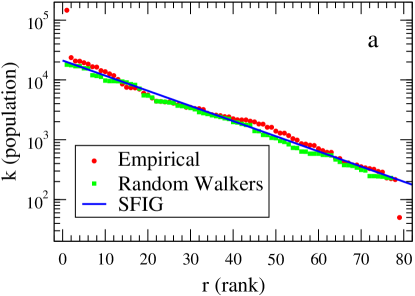
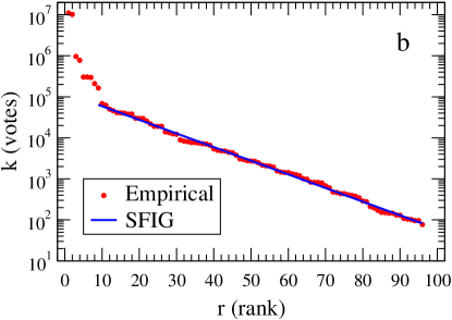
This behaviour, which corresponds to the class of universality $\gamma=0$ in (1), is that empirically found by Costa Filho et al. [8] in the distribution of votes in the Brazilian electoral results. We have found such a behaviour in i) the city-size distribution of small regions (as in the province of Huelva (Spain) [21]) and ii) electoral results (as in the 2008 Spanish General Elections results [22]). We depict in figures 1a and 1b the pertinent rank-sizes distributions in semi-logarithmic scale, where a straight line corresponds to a distribution of type (25). A large portion of the distributions can be fitted to (25), with a correlation coefficient of $0.994$ and $0.998$, respectively. From these fits we have obtain a bulk density of $\rho_{0}=0.058$ for the General Elections results, and in the case of Huelva of $\rho_{0}=17.1$ ($N=77$, $\Omega=4.5$). Using historical data for the later [21], we have used the backward differentiation formula to calculate the relative growth rate of the $i$-th city as

$$w_{i}=\frac{\ln k_{i}^{(2008)}-\ln k_{i}^{(2007)}}{\Delta t}$$ (26)

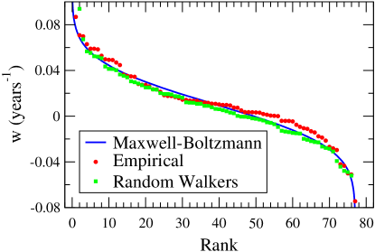
where $k_{i}^{(2007)}$ and $k_{i}^{(2008)}$ are the number of inhabitants of the $i$-th city in $2007$ and $2008$, respectively while $\Delta t=1$ year. We show in figure 2 the empirical rank-plot of the relative growth, where we have obtained $\overline{w}=0.011$ years^-1 and $\sigma_{w}=0.030$ years^-1, compared with the rank-plot of a Maxwell-Boltzmann distribution with the same mean value and standard deviation.

Figure 2: (colour on-line) Rank-plot of the growth rate $w$ of the province of Huelva between 2007 and 2008 (red dots) compared with a Boltzmann distribution with the same mean value and standard deviation (blue line).

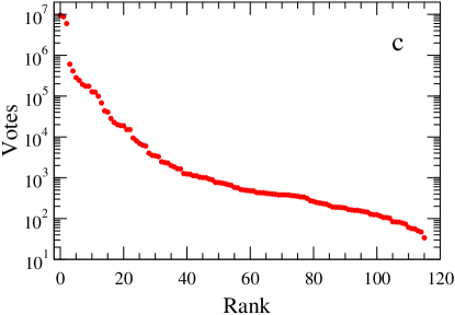
However, these regularities are not always obvious to the naked eye, as shown for the case of the most voted parties in Spain’08 or for the whole distribution of the 2005 General Elections results in the United Kingdom [23] (figure 1c). In both cases, the competition between parties seems to play an important role, and the assumption of non-interacting elements can be unrealistic .

5.1 Bulk and Zipf regimes

The situation in which $N/\Omega\rightarrow\,{\rm constant}\,\neq 0$ as $N,\Omega\rightarrow\infty$ will be referred to herefrom as the bulk regime. Now, in a recent communication [25], we show that Zipf’s law ($\gamma=1$ in (1) with a slope of $-1$ in the rank-plot) can be derived from the extremization of Fisher’s information with no constraints. In the thermodynamic context studied here, the absence of normalization can be understood as the inability of the system to reach the thermodynamic limit, i.e. $N/\Omega\rightarrow 0$ as $N,\Omega\rightarrow\infty$. In this case the system can not follow (24). Zipf’s law emerges as this behaviour of the density in what we will accordingly denominate the Zipf regime ($N/\Omega\rightarrow 0$). We digress on the conditions for both regimes in the example discussed below.

We have studied the system formed by all Physics journals [26] ($N=310$) using their total number of cites as coordinate $k$. If a journal receives more cites due to its popularity, it becomes even more popular and therefore it will receive more cites. Under such conditions proportional growth and scale invariance are expected. Since we consider all sub-fields of Physics, correlation effects are much lower than they would be should we only consider journals pertaining to an specific sub-field. Accordingly, the non-interacting approximation seems to be realistic in this instance. In figure 3 we depict the rank-plot of the number of citations in Physic journals, and find a slope approaching $-1$ for the most-cited journals in the logarithmic representation (figure 3a) and an slope in the vicinity of r $+1$ for the less-cited journals (figure 3b). For the central part of the distribution, the bulk density reaches a value of $\rho_{0}\sim 57$ (figure 3c).

Figure 3: (colour on-line) a, rank-plot of the total number of cites of physics journal, from most-cited to less-cited, in logarithm scale. b, sorted from less-cited to most cited c, same as a, in semi-logarithm scale. (Red dots: empirical data; blue line: fit to (25)).

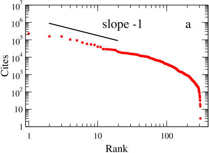
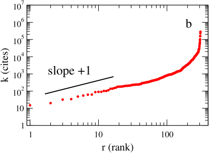
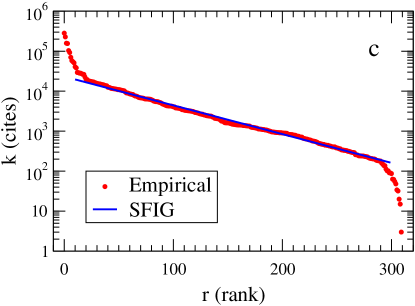
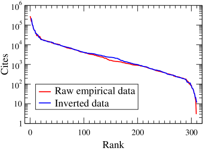
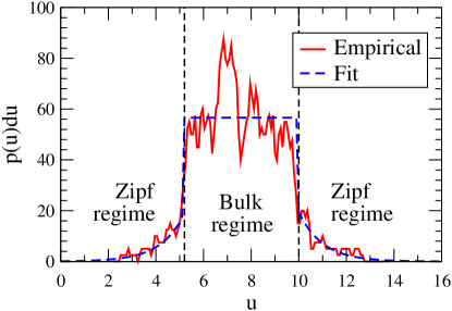
This distribution shows a notably symmetric behaviour under the change $k\rightarrow 1/k$ ($u\rightarrow-u$). We exhibit in figure 4 the raw empirical data as compared with the distribution obtained from the transformation $k^{\prime}=c/k$ ($u^{\prime}=-u+\ln c$), where $c=3.3\times 10^{6}$. The main part of the density distribution reaches the bulk density obeying (24), whereas Zipf’s law emerges at the edges, which could be understood as constituting the surface of the system, since they explain how the density (exponentially) falls from its bulk-value to zero in $u$-space when the system is exposed to an infinitely empty volume. This effect is clearly visible in figure 5, where the empirical density distribution $p(u)du$ in $u$-space is compared with the “fitted” density

$$p(u)=\left\{\begin{array}[]{ll}\rho_{Z}e^{u-u_{1}}&\mathrm{if~{}}u<u_{1}\\ \rho_{0}&\mathrm{if~{}}u_{1}<u<u_{2}\\ \rho_{Z}e^{u_{2}-u}&\mathrm{if~{}}u>2\end{array}\right.$$ (27)

where $\rho_{Z}=18$, $\rho_{0}=57$, $u_{1}=5.2$ and $u_{2}=10$. These findings lead us to conclude that the system consisting of Physics journals, when sorted by total number of citations, is a perfect example of a finite scale-free ideal gas at equilibrium.

Figure 4: (colour online) Rank-plot of the total number of cites of Physics journal, from most-cited to less-cited, compared with the distribution obtained from the inverse transformation $k^{\prime}=3.3\times 10^{6}/k$ where $k$ is the number of cites.

Figure 5: (colour online) Empirical density distribution in $u$-space of the total number of cites of Physics journals, compared with (27). The bulk regime and the Zipf regime at the edges is clearly visible.

5.2 An accompanying microscopic description

The dynamics of the system under scrutiny here can be microscopically described as a stochastic process using (13) together with the density distribution (21). Treating $w$ as a random variable, the pertinent stochastic equation of motion is written in the guise of a geometrical Brownian motion, i.e., [19]

$$dk=k\overline{w}dt+k\sigma_{w}dW,$$ (28)

where $dW$ represents a Wiener process. In the $u$-space, this equation reads

$$du=\overline{w}dt+\sigma_{w}dW,$$ (29)

and is known to describe the celebrated Brownian motion (28), which exactly describes the dynamical condition found empirically in [7] and also the (stochastic) proportional growth model used in [13] to obtain Zipf’s law. We thus dare to suggest that we are dealing here with a sort of “equivalent” of a molecular dynamics’ simulation for gases/liquids [27].

Indeed, (29) describes $N$ Brownian walkers moving in a fixed volume $\Omega$ with uniform density in $u$-space, a model used in the literature to describe the ideal gas [27]. This scenario can also be reproduced by our free-scale ideal gas merely by choosing to represent the system with the coordinates $(k,v)$. In figure 1a we show the rank-plot for $k$ of a system of $N=78$ geometrical Brownian walkers with $\overline{w}=0.011$ and $\sigma_{w}=0.030$ in a volume $\Omega=4.5$, with d $k_{1}=200$ in reduced units, which approximately describes the distribution of the population of the province of Huelva. We also show in figure 2 the rankplot of $w$ of the same random walkers, compared with the empirical data.

6 Conclusions

Our present considerations derive from the fact that, as shown in [14], thermodynamics can be reformulated in terms of the minimization with appropriate constraints of Fisher’s information. We have applied such reformulation in order to discuss the thermodynamics of scale-free systems and derived the density distribution in configuration space and the entropic expression for the equilibrium state of what we call SFIG: the scale-free ideal gas (in the thermodynamic limit). We have encountered convincing empirical evidences of the SFIG actual existence in sociological scenarios. Thus, we have dealt with city populations, electoral results and citations in Physics journals. In such a context it is seen that Zipf’s law emerges naturally as the equilibrium density of the non-interacting system when the volume grows without bounds, a situation that we call the Zipf regime. Using empirical data we have revealed that this regime can be understood as a density-decay at the “surface” separating the bulk from an empty and very large volume. Finally, we have shown with a simulation of city-populations that geometrical Brownian motion can describe such systems at a microscopic level.

References

- [1] Fractals in Physics: Essays in Honour of Benoit B Mandelbrot, edited by A. Aharony and J. Feder, Proceedings of a Conference in honor of B.B. Mandelbrot on His 65th in Vence, France, North Holland, Amsterdam, 1989.
- [2] K. Paech, W. Bauer, and S. Pratt , Phys. Rev. C 76 (2007), p. 054603; X. Campi and H. Krivine, Phys. Rev. C 72 (2005) 057602; Y. G. Ma et al., Phys. Rev. C 71 (2005) 054606.
- [3] C. Furusawa and K. Kaneko, Phys. Rev. Lett. 90 (2003) 088102.
- [4] G. K. Zipf, Human Behavior and the Principle of Least Effort, Addison-Wesley Press, Cambridge, Mass., 1949; I. Kanter and D. A. Kessler, Phys. Rev. Lett. 74 (1995) 4559.
- [5] M. E. J. Newman, Phys. Rev. E 64 (2001) 016131.
- [6] A.-L. Barabasi and R. Albert, Rev. Mod. Phys. 74 (2002) 47.
- [7] T. Maillart, D. Sornette, S. Spaeth, and G. von Krogh, Phys. Rev. Lett. 101 (2008) 218701.
- [8] R. N. Costa Filho, M. P. Almeida, J. S. Andrade, and J. E. Moreira, Phys. Rev. E 60 (1999) 1067.
- [9] A. A. Moreira, D. R. Paula, R. N. Costa Filho, and J. S. Andrade, Phys. Rev. E, 73 (2006) 065101(R).
- [10] L. C. Malacarne, R. S. Mendes, and E. K. Lenzi, Phys. Rev. E 65 (2001) 017106.
- [11] M. Marsili and Yi-Cheng Zhang, Phys. Rev. Lett. 80 (1998) 2741.
- [12] R. L. Axtell, Science 293 (2001) 1818.
- [13] X. Gabaix, Quarterly Journal of Economics 114 (1999) 739.
- [14] B. R. Frieden, A. Plastino, A. R. Plastino, and B. H. Soffer, Phys. Rev. E 60 (1999) 48; 66 (2002) 046128.
- [15] B. R. Frieden and B. H. Soffer, Phys. Rev. E 52 (1995) 2274; B. R. Frieden, Physics from Fisher Information, Cambridge University Press, Cambridge, England, 1998; B. R. Frieden, Science from Fisher Information, Cambridge University Press, Cambridge, 2004.
- [16] M. W. Zemansky and R. H. Dittmann,Heat and Thermodynamics, McGraw-Hill, London, 1981.
- [17] H. Goldstein, C. Poole and J. Safko, Classical Mechanics, 3rd Ed., Addison Wesley, San Francisco, 2002.
- [18] C. Cohen-Tannoudji, B. Diu and F. Laloe, Quantum Mechanics, Wiley-Interscience, New York, 2006.
- [19] W. J. Reed, and B. D. Hughes, Phys. Rev. E 66 (2002) 067103.
- [20] K. E. Kechedzhi, O. V. Usatenko, and V. A. Yampol’skii, Phys. Rev. E 72, 046138 (2005); S. Ree, Phys. Rev. E 73 (2006) 026115.
- [21] National Statistics Institute, Spain, www.ine.es.
- [22] Ministry of the Interior, Spain, www.elecciones.mir.es
- [23] Electoral Commission, Government of the UK, www.electoralcommission.org.uk.
- [24] A. Hernando, D. Villuendas, M. Abad and C. Vesperinas, arXiv:0905.3704v1, 2009.
- [25] A. Hernando, D. Puigdomenech, D. Villuendas, C. Vesperinas and A. Platino, submitted to Phys. Lett. A.
- [26] Journal Citation Reports (JCR) for 2007, Thomson Reuters.
- [27] Gould H and Tobochnik J 1996 An Introduction to Computer Simulation Methods: Applications to Physical Systems, 2nd Ed. (Addison-Wesley).