In this paper we study the BPS state counting in the geometry of local obstructed curve with normal bundle $\mathcal{O}\oplus\mathcal{O}(-2)$. We find that the BPS states have a framed quiver description. Using this quiver description along with the Seiberg duality and the localization techniques, we can compute the BPS state indices in different chambers dictated by stability parameter assignments. This provides a well-defined method to compute the generalized Donaldson-Thomas invariants. This method can be generalized to other affine ADE quiver theories.

1 Introduction

Recently there has been much progress in the D-branes BPS state index counting and its wall crossing behavior across the lines of marginal stabilities [1]. Physically the change in the BPS state index can be understood from the fact that in supergravity the separation of the multiple centered solution goes to infinity when the moduli approach the marginal stability wall [2]. This infinite separation causes the bound state to leave the Hilbert space and results in the discrete jumps in the BPS state spectrum.

On the other hand, we believe these BPS indices correspond to the generalized Donaldson-Thomas invariant defined in mathematical literatures [3][4]. In the generalized Donaldson-Thomas theory, the integration of the virtual fundamental class over the moduli space of the ideal sheaves is replaced by counting the stable objects in the derived category.

The physical interpretation of the wall crossing formula was given if we consider the BPS instanton corrections to the hyperkähler metric of the moduli space of 4d $N=2$ theory reduced on a circle [5]. The wall crossing formula is equivalent to the statement that this hyperkähler metric is continuous with respect to the moduli variation.

In [6] Szendrői considered the moduli space of the framed cyclic modules in the conifold path algebra. The torus fixed points in the moduli space are in one to one correspondence with the torus fixed ideals in the path algebra. With the knowledge that all the torus fixed ideal are generated by monomials, one could classify all the fixed points and arrange them into pyramid partitions of length 1 empty room configuration (ERC). These configurations can be summed exactly[7]. To find out the physical interpretation of Szendrői’s partition function, the authors in [8] used supergravity techniques and obtained the BPS spectra on a resolved conifold in all different chambers. In particular, the result in [6] was reproduced as a BPS state partition function in certain Kähler chamber. Later the authors in [9] found that the partition function of the pyramid partition with different ERC actually correspond to BPS state partition function in different chambers. They made conjecture about a new finite type pyramid partitions, which will asymptote to the stable pair invariant (aka Pandharipande-Thomas or PT invariant) [10] when the length of the ERC goes to infinity. The conjecture was later proven by [11].

This relation between the different ERCs and Kähler chambers arises if we start from the original framed conifold quiver and then perform the Seiberg duality to bring back the stability parameters (FI parameters) to the cyclic FI parameter assignment. This mutation, or Seiberg duality in physics term, will result in the change in the framing data and superpotential. From new framing data and new superpotential, one determines the new ERC for the pyramid partitions.

The Seiberg duality of the quiver theory sometimes simply provides us different aspects of the same thing. In this case, however, after the mutation it will become extremely easy to visualize the arrangement of the torus fixed points in the cyclic chamber of the mutated quiver with new framing data and new superpotential.

In this paper we consider a local obstructed $\mathbb{P}^{1}$ with normal bundle $\mathcal{O}\oplus\mathcal{O}(-2)$. The quiver theory with superpotential was given in [12]. The superpotential deformation is determined by the obstruction of the $\mathbb{P}^{1}$. In order to study the D6-D2-D0 system on this geometry we introduce a framing node into the quiver. We find that the mutated quiver in the cyclic chamber computes what the original framed quiver in certain chamber does. In other words, due to the simplicity of the cyclicity, we can bring the quiver theory back to the cyclic chamber by using Seiberg duality, which will change the new superpotential and the arrow structure connecting the framing node.

We then consider the framed cyclic $\mathcal{A}$-module of the mutated quiver, where $\mathcal{A}$ is the path algebra of the mutated quiver. In this quiver theory there are still $(\mathbb{C}^{*})^{2}$ actions leaving F-term relations invariant, although the geometry is nontoric. Once again the torus fixed point in the moduli space of the framed cyclic $\mathcal{A}$-module should be in one-to-one correspondence with the torus fixed ideals of the path algebra. These ideals are generated by monomials and can be arranged into filtered pyramid partitions of $(n,k)$ (in)finite ERC, where $n$ is the degree of the obstruction in the geometry and $k$ is the number of the framing arrows.

After the classification we can utilize the localization techniques to compute the contribution from each fixed point. Unlike conifold in which the $(\mathbb{C}^{*})^{2}$ actions preserve the superpotential, the deformation complex is not self-dual in this case. Therefore the local contribution of each fixed point will be generically a rational function in terms of localization parameters. After summing all the fixed points for a given dimension vector assignment we find the integrability is recovered.

Since the local obstructed $\mathbb{P}^{1}$ geometries can be deformed into $n$ isolated conifold geometries by using complex deformation and every $\mathbb{P}^{1}$ is homologous to each other, we expect the localization result should reproduce $n$ copies of the conifold. We compare our result with this expectation and find perfect match.

The paper is organized as follows. In section 2 we introduce the geometry on which we will study the BPS state counting. Section 3 is about the Seiberg duality in affine $A_{1}$ quiver and what this mutated framed quiver computes. In section 4 we classify all the torus fixed points in the mutated framed affine $A_{1}$ quiver by looking for toric fixed annihilator ideals. In section 5 we comment on the implication for the melting crystal model. In section 6 we conclude and discuss some possible future directions. In appendix ABCD we give a short review on the mutation and present the new result about the mutation on a quiver theory with framing and adjoint fields. Appendix E contains the explicit construction of the deformation complex and useful information for computing the local contributions of the torus fixed points.

2 The Geometry: A $\mathbb{P}^{1}$ with Obstruction

The main geometry discussed in this paper is a local obstructed $\mathbb{P}^{1}$. Such local $\mathbb{P}^{1}$ can be described explicitly in patches with transition functions [12] [13]:

$$w = x^{-1}$$

$$z_{1} = x^{2}y_{1}+xy_{2}^{n}$$

$$z_{2} = y_{2}$$ (2.1)

where $(n+1)$ is the degree of the obstruction.

Define a map from these two patches $(w,z_{1},z_{2})$ and $(x,y_{1},y_{2})$ to $\mathbb{C}^{4}$:

$$v_{1}=z_{2}=y_{2},\ \ \ v_{2}=z_{1}=x^{2}y_{1}+xy_{2}^{n},$$

$$v_{3}=wz_{1}=xy_{1}+y_{2}^{n},\ \ \ v_{4}=w^{2}z_{1}-wz_{2}^{n}=y_{1}.$$ (2.2)

Then the geometry is defined by $v_{2}v_{4}-v_{3}^{2}+v_{3}v_{1}^{n}=0$ in $\mathbb{C}^{4}$, or by a change of coordiantes, $u_{1}^{2}+u_{2}^{2}+u_{3}^{2}+u_{4}^{2n}=0$ in $\mathbb{C}^{4}$.

The quiver theory can be obtained by performing an Ext group computation and using the $A_{\infty}$ structure [12].

(2.3)

The superpotential is,

$$W=w(C_{1})-w(C_{2})+C_{1}(B_{1}A_{1}+B_{2}A_{2})-C_{2}(A_{1}B_{1}+A_{2}B_{2}),$$ (2.4)

where $w(C_{i})=\frac{1}{n+1}C_{i}^{n+1}$.

Taking partial derivatives of $W$ gives the following relations:

$$C_{1}^{n}+B_{1}A_{1}+B_{2}A_{2}=0$$

$$C_{2}^{n}+A_{1}B_{1}+A_{2}B_{2}=0$$

$$C_{1}B_{i}=B_{i}C_{2}$$

$$C_{2}A_{i}=A_{i}C_{1}.$$ (2.5)

First note that we get the same relation as $n=1$ (Klebanov-Witten) by commuting $C_{i}$ k times through $A_{i}$ and $B_{i}$

$$A_{i}C_{1}^{k} =C_{2}^{k}A_{i}$$

$$B_{i}C_{2}^{k} =C_{1}^{k}B_{i}$$ (2.6)

and plugging the relation (2) back into (2):

$$A_{1}B_{i}A_{2} =A_{2}B_{i}A_{1}$$

$$B_{1}A_{i}B_{2} =B_{2}A_{i}B_{1}$$ (2.7)

One may identify the center of the algebra by:

$$\begin{split}x&=A_{1}B_{1}+B_{1}A_{1}-A_{2}B_{2}-B_{2}A_{2}\\ y&=2(A_{1}B_{2}+B_{2}A_{1})\\ z&=2(A_{2}B_{1}+B_{1}A_{2})\\ u&=C_{1}+C_{2}\end{split}$$ (2.8)

which satisfies:

$$x^{2}+yz-u^{2n}=0$$ (2.9)

Namely the center of the path algebra of the quiver (2.3) is the same geometry we are looking at. For a generic superpotential deformation $w(C_{i})=\frac{1}{n+1}C_{i}^{n+1}+a_{n}C_{i}^{n}+\cdots$, we can repeat this and obtain the center of the path algebra as $x^{2}+yz-(w^{\prime}(u))^{2}=0$.

Recall that each node of the quiver represents an object in the derived category of coherent sheaves. In this case the objects are $\mathcal{O}_{C}$ and $\mathcal{O}_{C}(-1)[1]$ respectively. This quiver is also called as unframed affine $A_{1}$ quiver with degree $n+1$ superpotential deformation. In the next section we will add a framing node (D6 node) into this quiver theory and impose the stability condition.

3 Framed Affine $A_{1}$ Quiver with Superpotential Deformation

Since our goal is to count D6-D2-D0 bound states in the local geometry (2), we need to introduce a new node for $D6$ brane wrapping the whole geometry and then impose certain stability condition. In the quiver theory the stability condition is imposed by assigning FI parameters to each node in the quiver. Counting BPS states is equivalent to counting the stable representation of the quiver theory under this FI parameter assignment [17]. A commonly used stability condition is to require the representations of the quiver theory to be cyclic. That is to say, every representation is generated by a vector field $\mathbb{C}$ in the vector space $V_{1}$ at node 1.

The added node for $D6$ brane represents the structure sheaf $\mathcal{O}_{X}$ and the resulting quiver theory is as follows.

(3.1)

By some simple argument we can show that cyclicity implies that the FI parameter $\theta_{0}$ for the D6 node is positive which other FI parameters are negative [9]. Note that, if the degree $n=1$, we can integrate out $C_{1}$ and $C_{2}$ in the superpotential and reproduce the conifold quiver [18]. Such a conifold quiver in the cyclic chamber will compute the noncommutative Donaldson-Thomas invariant a là Szendrői. In Szendrői partition function the MacMahon factor is present, which signals the noncompactness of the moduli space. The physical interpretation is that in general the D0-branes do not have to be bound to the D2-branes.

In fact we would like to find a chamber, dictated by the assignment of the $\theta$s, describing the PT chamber. The PT invariants are supposed to be the same as DT or GW invariant, modulo the MacMahon. Such a chamber in conifold quiver was actually found in [9][11]. In order to get to such a chamber, we have to start from a different quiver theory with a reversed framing arrow in the cyclic chamber and still keep $\theta_{0}$ positive. The cyclic chamber for this reversed framed quiver is actually an empty chamber, in which every representation is unstable.

Relevant digression (Conifold example) : Since we will borrow some of the conifold results, we give a brief review on it now. The framed conifold quiver in NCDT chamber is given by the following quiver with the usual quartic superpotential and $\theta_{0}>0$, $\theta_{1},\theta_{2}<0$:

(3.2)

$$W=A_{1}B_{1}A_{2}B_{2}-A_{1}B_{2}A_{2}B_{1}$$ (3.3)

If we keep the same $\theta$ parameter assignment and reverse $Q_{1}$, we obtain a quiver theory of which the generating function is simply 1, due to the fact mentioned in the footnote.

(3.4)

The PT chamber is actually described by this quiver theory with $\theta_{1}$ and $\theta_{2}$ being very close to the 45 degree line in the $\theta_{1}$-$\theta_{2}$ plane [11]. See Fig.1 for details.

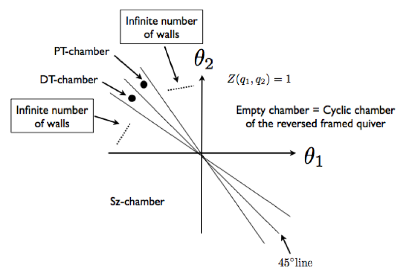
Figure 1: This is the chamber structure of the original conifold quiver with only one framing arrow.

However we can use the Seiberg duality to get a mutated quiver with cyclic $\theta$ assignment. In the mutated quiver the number of framing arrows will increase to number $k$ as illustrated below.

(3.5)

Under the mutation at node 2, the $\theta$ parameters will change in the following way[19]:

$$\theta_{1}\rightarrow\theta_{1}+2\theta_{2},\ \ \theta_{2}\rightarrow-\theta_{2}.$$ (3.6)

After alternating $k$ steps of the mutations, the $\theta$ parameters of the mutated quiver $(\tilde{\theta}_{1},\tilde{\theta}_{2})$ is related to the $\theta$ parameters of the original quiver as follows:

$$\tilde{\theta}_{1}=k\theta_{1}+(k+1)\theta_{2},\ \ \tilde{\theta}_{2}=-((k-1)\theta_{1}+k\theta_{2}).$$ (3.7)

The cyclic chamber of the mutated quiver defined by $(\tilde{\theta}_{1}<0,\tilde{\theta}_{2}<0)$ is actually a small chamber in Fig.1 given by

$$k\theta_{1}+(k+1)\theta_{2}<0,\ \ (k-1)\theta_{1}+k\theta_{2}>0.$$ (3.8)

The partition function will be the PT invariants truncated at certain D2 and D0 charges determined by $k$.

$$\mathbb{Z}(u,v)=\prod_{i=1}^{k}(1-(-u)^{i}v^{-1})^{i}$$ (3.9)

Therefore if we take large $k$ limit the partition function will approach the PT invariants. $\spadesuit$

The starting point will be the reversed framed quiver with $\theta_{0}>0$ and $\theta_{1},\theta_{2}<0$ as follows:

(3.10)

The other advantage to start from this empty chamber is that the Seiberg duality (mutation) can be performed more easily, which will be explained in the appendix. The mutation in such quiver is realized in a very similar way like conifold. Here is a simple illustration of the mutation. A more detailed treatment on the mutation on affine $A_{1}$ is given in appendix. We simply quote the result here.

(3.11)

The superpotential for the LHS quiver is given by

$$W=w(C_{1})-w(C_{2})+C_{1}(B_{1}A_{1}+B_{2}A_{2})-C_{2}(A_{1}B_{1}+A_{2}B_{2})+B_{1}P_{1}Q_{1}+B_{2}P_{1}Q_{2},$$ (3.12)

while the superpotential for the RHS quiver is

$$\tilde{W}=w(\tilde{C}_{1})-w(\tilde{C}_{2}) + \tilde{C}_{1}(\tilde{B}_{1}\tilde{A}_{1}+\tilde{B}_{2}\tilde{A}_{2})-\tilde{C}_{2}(\tilde{A}_{1}\tilde{B}_{1}+\tilde{A}_{2}\tilde{B}_{2})+$$ (3.13)

$$\tilde{P}_{1}\tilde{A}_{1}\tilde{Q}_{1}+\tilde{P}_{2}(\tilde{A}_{2}\tilde{Q}_{1}-\tilde{A}_{1}\tilde{Q}_{2})+\tilde{P}_{3}\tilde{A}_{2}\tilde{Q}_{2}$$

More generically, we have the mutation from $k$ to $k+1$:

(3.14)

The superpotentials are

$$W = w(C_{1})-w(C_{2})+C_{1}(B_{1}A_{1}+B_{2}A_{2})-C_{2}(A_{1}B_{1}+A_{2}B_{2})+$$ (3.15)

$$Q_{1}B_{1}P_{1}+Q_{2}(B_{2}P_{1}-B_{1}P_{2})+Q_{3}(B_{2}P_{2}-B_{1}P_{3})+\cdots+Q_{k+1}B_{2}P_{k}$$

$$\tilde{W} = w(\tilde{C}_{1})-w(\tilde{C}_{2})+\tilde{C}_{1}(\tilde{B}_{1}\tilde{A}_{1}+\tilde{B}_{2}\tilde{A}_{2})-\tilde{C}_{2}(\tilde{A}_{1}\tilde{B}_{1}+\tilde{A}_{2}\tilde{B}_{2})+$$ (3.16)

$$\tilde{P}_{1}\tilde{A}_{1}\tilde{Q}_{1}+\tilde{P}_{2}(\tilde{A}_{2}\tilde{Q}_{1}-\tilde{A}_{1}\tilde{Q}_{2})+\tilde{P}_{3}(\tilde{A}_{2}\tilde{Q}_{2}-\tilde{A}_{1}\tilde{Q}_{3})+\cdots+\tilde{P}_{k+2}\tilde{A}_{2}\tilde{Q}_{k+1}$$

This local obstructed $\mathbb{P}^{1}$ geometry can be resolved into $n$ isolated conifold points and all the n $\mathbb{P}^{1}$s are homologous to each other. Recall that the authors in [12] choose the same basis for this geometry as the conifold in the Ext group computation. Under the mutation the $\theta$ parameters should also change according to (3.6). Moreover, one can perform a similar wallcrossing analysis as [8] and should obtain the same chamber structure.

With all the pieces of information, our educational expectation would be that in every chamber the BPS states partition function should be n-th power of that of the conifold. In the next section we will classify all the fixed points in the moduli space.

4 Classification of the Torus Fixed Points

In this section we classify all the torus fixed points in the moduli space. As we will see later the ERC is $n$ copies of conifold ERC of length $k$. We denote this ERC by ”$(n,k)$ (in)finite ERC” for short. We find that the fixed points are classified by filtered pyramid partitions of $(n,k)$ (in)finite ERC. At first glance, it seems strange because we really want $n$ independent copies of the conifold answer. If the fixed points are classified by filtered partitions and the partitions are correlated, how can we reproduce the desirable answer?

But we have to be more careful here because the torus actions in the geometry only fix invariant the F-term relations, not the superpotential itself, which renders the deformation complex not symmetric and self-dual. Because of this the local contribution is actually not simply $(-1)^{\text{dim}T_{f}\mathcal{M}}$ but rather a rational function of the localization parameters. In the end we will show by examples that the integrability reappear after grouping together all the fixed points with same dimension vectors.

Consider the torus action on moduli space $\mathcal{M}_{\textbf{v}}$ of framed, cyclic representations of $\mathcal{A}$ with a single framing $m$, where $\vec{v}=(v_{1},v_{2})$ is the dimension vector:

$$\begin{split}(t_{1},t_{2})\in(C^{*})^{2}:\mathcal{A}&\rightarrow\mathcal{A}\\ (A_{1},A_{2},B_{1},B_{2},C_{1},C_{2})&\mapsto(t_{1}^{-1}t_{2}^{n}A_{1},t_{1}t_{2}^{n}A_{2},t_{1}B_{1},t_{1}^{-1}B_{2},t_{2}C_{1},t_{2}C_{2})\end{split}$$ (4.1)

Proposition The fixed points under torus actions above are isolated and classified by filtration of pyramid partitions of $(n,k=1)$ infinite ERC. The $(n,k=1)$ infinite ERC is shown in Fig.2.

Proof: Denote the Klebanov-Witten quiver path algebra $\mathcal{A}_{c}$ which only involves $A_{i}$ and $B_{i}$ and has the same relation (2). Note that the algebra $\mathcal{A}$ is $\mathbb{Z}_{n}$-graded by the power of $C_{i}$, one can always move $C_{i}$ to the very left by using (2).

$$\mathcal{A}=\bigoplus_{k=0}^{n-1}\mathcal{A}_{k}=\bigoplus_{k=0}^{n-1}(C_{1}+C_{2})^{k}\mathcal{A}_{c}$$ (4.2)

There is a natural projection $\pi_{k}:\mathcal{A}_{k}\rightarrow\mathcal{A}_{c}$. So is the framed cyclic module $M$:

$${M=\bigoplus_{k=0}^{n-1}M_{k}}$$ (4.3)

where $M_{k}=(C_{1}+C_{2})^{k}M_{c}$ for some framed $\mathcal{A}_{c}$-module $M_{c}$ with the same framing $m$.

By a similar argument as in [6], one can show that the fixed point is in 1-1 correspondence with the $m$-annihilator ideal of $Q$ generated by monomial:

$$\mathcal{A}\supset I=\bigoplus_{k=0}^{n-1}I_{k}$$ (4.4)

If $\alpha\in I_{k}$, then $(C_{1}+C_{2})\alpha\in I_{k+1}$. Thus we conclude:

$$\pi_{1}I_{1}\subset\pi_{2}I_{2}\subset\cdots\subset\pi_{k}I_{k}\subset\cdots$$ (4.5)

Moreover each $I_{k}$ is classified by a pyramid partition consisting of black and white stones denoting one-dimensional subspaces of given toric weights [6]. Roughly speaking $I_{k}$ tells how to truncate an infinite pyramid partition from below, therefore we conclude that the fixed point corresponds to a nested pyramid partition of length $n$, where the sum of all white(black) stones is $v_{1}$($v_{2}$).

For mutated quiver, we have similar torus action:

$$(A_{1},A_{2},B_{1},B_{2},C_{1},C_{2},P_{1},P_{2},\dots,P_{k},Q_{1},Q_{2},\dots,Q_{k+1})$$ (4.6)

having weights

$${(\underbrace{t_{1}^{-1}t_{2}^{n},t_{1}t_{2}^{n}}_{A_{1},A_{2}},\underbrace{t_{1},t_{1}^{-1}}_{B_{1},B_{2}},\underbrace{t_{2},t_{2}}_{C_{1},C_{2}},\underbrace{1,t_{1}^{2},t_{1}^{4},\dots}_{P_{1},...,P_{k}},\underbrace{t_{1}t_{2},t_{1}^{-1}t_{2},t_{1}^{-3}t_{2},\dots}_{Q_{1},...,Q_{k+1}})}$$ (4.7)

The algebra is also graded, but this time we have to impose cyclicity first to kill the $Q_{i}$’s, then one can similarly project to subalgebra of mutated conifold quiver, whose torus fixed points are classified by finite pyramid partition. Thus we conclude:

Proposition Mutated quiver at step $k$ has a torus action whose fixed points are classified by filtration of pyramid partitions of $(n,k)$ (in)finite ERC. Fig.3 shows the $(n,3)$ finite ERC. Fig.4 represents a fixed point in $(n,3)$ finite ERC.

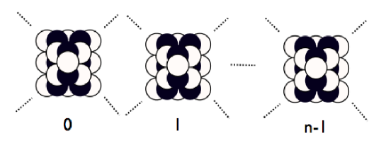
Figure 2: This is the ERC for affine $A_{1}$ quiver with superpotential degree (n+1) and 1 framing arrows, which is not reversed. It is denoted by $(n,1)$ infinite ERC.

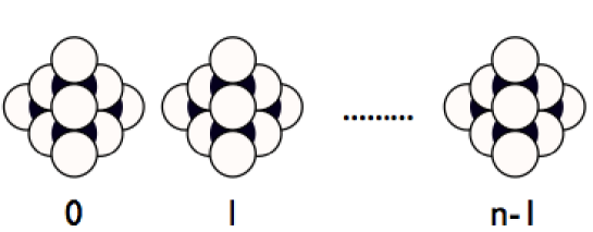
Figure 3: This is the ERC for affine $A_{1}$ quiver with superpotential degree (n+1) and 3 framing arrows, denoted by $(n,3)$ finite ERC.

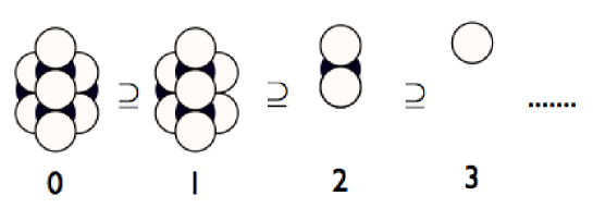
Figure 4: An example of the filtered pyramid partitions of $(n,3)$ finite ERC. ($n\geq 3$)

Now we provide some examples with different dimension vectors $\vec{v}$ and general value of $n$. The basis of the quiver with $k$ framing arrows is ${\mathcal{O}_{C}(-k-1)[1],\mathcal{O}_{C}(-k-2)}$. Translating it into brane charges we have $\{D2+(k+1)\ \bar{D0},\bar{D2}+k\ D0\}$. We then denote $\Gamma=(\bar{D2}\ \text{charge},D0\ \text{charge}).$

Example 1    $k=2$, general $n$, $\vec{v}=(1,0)$, $\Gamma=(1,2)$. Two fixed points are $p_{1}=\{V_{1}=1,V_{2}=0\}$ and $p_{2}=\{V_{1}=t_{1}^{-2},V_{2}=0\}$. The deformation complex (E.3)(E.4) simplifies to

$$0\rightarrow \text{Hom}(V_{1},V_{1})\rightarrow\text{Hom}(V_{1},V_{1}\otimes t_{2})\oplus\text{Hom}(\mathbb{C},V_{1})\oplus\text{Hom}(\mathbb{C},V_{1}\otimes t_{1}^{2})\rightarrow$$ (4.8)

$$\text{Hom}(V_{1},V_{1}\otimes t_{2}^{n})\oplus\text{Hom}(V_{1},\mathbb{C}\otimes t_{2}^{n+1})\oplus\text{Hom}(V_{1},\mathbb{C}\otimes t_{1}^{-2}T_{2}^{n+1})\rightarrow$$

$$\text{Hom}(V_{1},V_{1}\otimes t_{2}^{n+1})\rightarrow 0$$

Abusing the notation, we first compute

$$\mathcal{T}=\mathcal{T}_{0}-\mathcal{T}_{1}+\mathcal{T}_{2}-\mathcal{T}_{3}=V_{1}^{*}\otimes V_{1}(1-t_{2}+t_{2}^{n}-t_{2}^{n+1})-V_{1}(1+t_{1}^{2})+V_{1}^{*}(1+t_{1}^{-2})t_{2}^{n+1}.$$ (4.9)

for each of the fixed point and then perform the substitution

$$\mathcal{T}=\sum k_{(n_{1},n_{2})}t_{1}^{n_{1}}t_{2}^{n_{2}}\to P(\alpha_{1},\alpha_{2})=\prod(n_{1}\alpha_{1}+n_{2}\alpha_{2})^{k_{(n_{1},n_{2})}}.$$ (4.10)

In this case

$$P_{p_{1}}=-n+\frac{n+1}{2}\frac{\alpha_{1}}{\alpha_{2}}$$ (4.11)

$$P_{p_{2}}=-n-\frac{n+1}{2}\frac{\alpha_{1}}{\alpha_{2}}$$ (4.12)

. (4.13)

Therefore, we obtain the Euler character of the moduli space

$$e(\mathcal{M}_{(1,2)})=-2n.$$ (4.14)

Here we specify the moduli by the Dbrane charges for later convenience.

Example 2   Fig. 5. $k=2$, general $n$, $\vec{v}=(2,0)$, $\Gamma=(2,4)$. We find three fixed points: $p_{1}=\{V_{1}=1+t_{1}^{-2},V_{2}=0\}$, $p_{2}=\{V_{1}=1+t_{2}^{-1},V_{2}=0\}$ and $p_{3}=\{V_{1}=t_{1}^{-2}+t_{1}^{-2}t_{2}^{-1},V_{2}=0\}$ The final result is

$$e(\mathcal{M}_{(2,4)})=-n+2n^{2}.$$ (4.15)

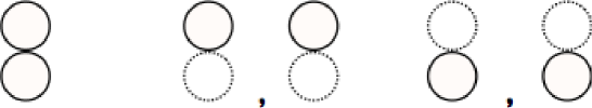
Figure 5: This figure shows the three fixed point in Example 2.

Example 3   Fig. 6. $k=2$, general $n$, $\vec{v}=(2,1)$, $\Gamma=(1,1)$. The single fixed in this case is $p_{1}=\{V_{1}=1+t_{1}^{-2},V_{2}=t_{1}^{-1}\}$. This is the first nontrivial example in which $V_{2}\neq 0$. We have to use the whole complex (E.3) (E.4) and obtain,

$$e(\mathcal{M}_{(1,1)})=n.$$ (4.16)

Figure 6: The single fixed point for dimension vector $\vec{v}=(2,1)$.

Example 4   Fig. 7. $k=2$, general $n$, $\vec{v}=(3,0)$, $\Gamma=(3,6)$ $p_{1}=\{V_{1}=1+t_{1}^{-2}+t_{2}^{-1},V_{2}=0\}$, $p_{2}=\{V_{1}=1+t_{1}^{-2}+t_{1}^{-2}t_{2}^{-1},V_{2}=0\}$, $p_{3}=\{V_{1}=1+t_{2}^{-1}+t_{2}^{-2},V_{2}=0\}$, $p_{3}=\{V_{1}=(1+t_{2}^{-1}+t_{2}^{-2})t_{1}^{-2},V_{2}=0\}$.

$$e(\mathcal{M}_{(3,6)})=-\frac{2n(2n-1)(2n-2)}{6}.$$ (4.17)

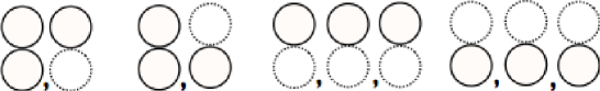
Figure 7: 4 fixed points for $\vec{v}=(3,0)$.

Compare with the expected result. Now let us compare these examples with the expected answers. Partition function for cyclic representations of that mutated conifold quiver with $k$ framing arrows is[9]

$$\mathcal{Z}^{\text{conifold}}_{k}=\sum_{p,q}D(p,q)u^{q}v^{p}=\prod_{j=1}^{k}(1-(-u)^{j}v)^{j}$$ (4.18)

where $D(p,q)$ is the virtual Euler character of quiver moduli space of $\bar{D2}/D0$ charge $(p,q)$. In affine $A_{1}$ quiver with superpotential deformation $w(C_{i})$ of degree $n+1$, we expect to get

$$\mathcal{Z}^{w}_{k}=(Z^{\text{conifold}}_{k})^{n}=\prod_{j=1}^{k}(1-(-u)^{j}v)^{jn}.$$ (4.19)

In the explicit examples presented above, we all have $k=2$. Therefore we should compare them with the following:

$$\mathcal{Z}_{k=2}= (1-(-u)v)^{n}(1+u^{2}v)^{2n}=(1+nuv+\binom{n}{2}u^{2}v^{2}+\binom{n}{3}u^{3}v^{3}+\cdots)$$ (4.20)

$$(1-2nu^{2}v+\binom{2n}{2}u^{4}v^{2}-\binom{2n}{3}u^{6}v^{3}+\cdots)$$

The Euler characters of the examples can be read off as follows:

$$e(\mathcal{M}_{(1,2)})=-2n,\ \ e(\mathcal{M}_{(2,4)})=-n+2n^{2},\ \ e(\mathcal{M}_{(1,1)})=n,\ \ e(\mathcal{M}_{(3,6)})=-\frac{2n(2n-1)(2n-2)}{6}.$$ (4.21)

These computations provide strong favorable evidences for our classification of the fixed points.

5 A New Type of Melting Crystal Model?

The statistical model of the melting crystal model was first proposed as a realization of quantum gravitational path integral over the fluctuations of the Kähler geometries [20].

Recently there are again many activities in constructing the statistical model of melting crystal to count the BPS state bound states in noncompact Calabi-Yau manifolds. The smooth classical emerges as a thermodynamic limit of the statistical mechanical model of crystal melting [21]. Mathematically speaking, each atoms or melting crystal configuration corresponds to a torus fixed point in the moduli space of the quiver representation. Since the geometry is toric, every fixed point should contribute either $+1$ or $-1$, depending on the dimension vector of the quiver theory.

In our example, we find the weights of the fixed point are rational functions, rather than integers. This suggests there should exist a large class of melting crystal model with more general weights. There exist many other obstructed local $\mathbb{P}^{1}$ geometries, which are not toric and have two natural $(\mathbb{C}^{*})^{2}$ actions. For example, we can construct obstructed local $\mathbb{P}^{1}$ with normal bundle $\mathcal{O}(1)\oplus\mathcal{O}(-3)$ by gluing two patches of $\mathbb{C}^{3}$, with coordinates $(x,y_{1},y_{2})$ and $(w,z_{1},z_{2})$ by the following transition functions[13]:

$$z_{1}=x^{3}y_{1}+y_{2}^{2}+x^{2}y_{2}^{2n+1},\ \ \ z_{2}=y_{2}/x,\ \ \ w=1/x.$$ (5.1)

It would be also interesting to study the BPS state counting in this class of geometries and say something useful about the weight assignment in the study of quantum geometries.

6 Conclusion

In this paper we study the BPS state counting in the geometry of local obstructed curve with normal bundle $\mathcal{O}\oplus\mathcal{O}(-2)$. We find that the D6-D2-D0 bound states have a framed affine $A_{1}$ quiver description with degree $(n+1)$ superpotential deformation.

We then develop a new way to mutate this framed quiver with adjoint fields and obtain the new superpotential and the new framing structure after the mutation. The mutation on the quiver with both adjoint fields and framing is nontrivial and is presented in Appendix ABCD. Using this quiver description along with the mutation, we can bring the original framed quiver in any chambers to a certain mutated quiver in the cyclic chamber.

The new superpotential and cyclicity in the mutated quiver will simplify dramatically the classification of the fixed points. We find that the fixed points are classified by filtered pyramid partitions of $(n,k)$ (in)finite ERC. We verify this classification by doing explicit computations of the local contributions of the fixed points. In this nontoric geometry, the deformation complex will cease to be selfdual and therefore the integrability only appears after grouping together the fixed points with the same dimension vector.

This method of mutating back to the cyclic chamber provides a well-defined method for computing generalized Donaldson-Thomas invariant in different chambers. This general idea can be generalized to other affine ADE quiver theories. We present some affine $A_{n}$ results in the appendix D and leave the DE-type cases for future study. Finally we comment on the implications on the melting crystal models and mention possible future directions.

Acknowledgments: We would like to thank Emanuel Diaconescu for suggesting the problem and for his patient guidance throughout the project. WYC and GP are supported by DOE grant DE-FG02-96ER40959.

In the appendix we first briefly review the procedure for performing the mutation to the quiver theory. After that we give explicit examples of the mutation for affine A-type quiver without and with framing. We find that the mutation of the affine $A_{1}$ quiver with superpotential deformations works pretty much the same way as the conifold [9]. The mutation of affine $A_{n}$ quiver is given in the subsequent section. We then give the deformation complex for the affine $A_{1}$ case to compute the local contribution of the torus fixed points.

Appendix A Seiberg Duality and Mutation

The section is a crash review on the mutation, following [22]. The Seiberg duality or mutation on quiver theory is a tilting procedure and therefore is an equivalence of the derived categories. In order to check if a complex is tilting one needs to compute the morphisms in the homotopy category between the objects, namely, the complex formed by the projective objects.

First consider a quiver with superpotential and let $\mathcal{A}$ be the path algebra of the quiver and $\mathcal{Q}$ the abelian category of $\mathcal{A}$-module. Let $K^{b}(\mathcal{Q})$ be the homotopy category, where the morphisms are the homotopy classes of the chain maps. A tilting complex over $\mathcal{A}$ is an object $T$ in $K^{b}(\mathcal{Q})$, satisfying the following two properties:

• $Hom_{K^{b}(\mathcal{Q})}(T,T[n])=0$ for all $n\neq 0$.

• $T$ generates $K^{b}(\mathcal{Q})$ as a triangulated category.

Our procedure for performing the mutation on framed affine $A_{n}$ quiver theory at k-th vertex, where the framing arrows are outgoing, is to replace the one term complex at k-th vertex

$$0\rightarrow\underline{\mathcal{P}_{k}}\rightarrow 0$$

by

$$0\rightarrow\underline{\oplus_{j\to k}\mathcal{P}_{j}}\rightarrow\mathcal{P}_{k}\rightarrow 0$$

where the underline means the zeroth position of the complex and $\mathcal{P}_{k}$ is the projective module consisting of all the paths in the path algebra ending on $k$-th node. It is easy to check that it is projective.

In this case we define the tilting complex

$$T=\oplus_{i=1}^{n}T_{i}$$

where

$$T_{i}:\ \ 0\rightarrow\underline{\mathcal{P}_{i}}\rightarrow 0,\ \ i\neq k$$

$$T_{k}:\ \ 0\rightarrow\underline{\oplus_{j\to k}\mathcal{P}_{j}}\rightarrow\mathcal{P}_{k}\rightarrow 0$$ (A.1)

Most of the morphisms in $Hom_{K^{b}(\mathcal{Q})}(T,T[n])$ are trivial up to the homotopy except the following two diagrams, which potentially might represent certain nontrivial morphisms in $Hom_{K^{b}(\mathcal{Q})}(T,T[n])$.

(A.2)

(A.3)

(A.2) is used to compute $Hom(T_{k},T_{i}[-1])$, while (A.3) is the element in $Hom(T_{k},T_{k}[-1])$.

A morphism in $Hom(T_{k},T_{i}[-1])$ means a mapping $\alpha:\mathcal{P}_{k}\to\mathcal{P}_{i}$ such that for every mapping $\beta:\oplus_{j\to k}\mathcal{P}_{j}\to\mathcal{P}_{k}$ we have $\beta\circ\alpha=0$, do to the commutativity of the diagram (A.2). This condition is very restricted and we can not find such morphisms in affine $A_{n}$ quiver, if we perform the mutation at the node with outgoing framing arrows. The second tilting property can be easily verified too.

Appendix B A-type Quiver without Framing

Although Seiberg duality with adjoint fields has been studied in [23] [24], their procedures are not exactly applicable for our purpose. We find that we have to resort to the reflection operation in [25] [26] and make suitable adjustment due to the presence of the new framing arrows. In this section we will present the reflection operation in terms of the aforementioned tilting complex. We consider the affine $A_{2}$ quiver without framing:

(B.1)

$X_{ij}$ denotes the mapping from $j$-th node to $i$-th node. And $C_{i}$ is the adjoint field at $i$-th node. The relations are given by [26]

$$X_{i,i-1}X_{i-1,i}-X_{i,i+1}X_{i+1,i}=w_{i}(C_{i})$$ (B.2)

$$X_{ij}C_{j}=C_{i}X_{ij}$$ (B.3)

$$\sum_{i}d_{i}w_{i}=0,\ \ \text{$d_{i}$:Dynkin index at i-th node.}$$ (B.4)

Let us mutate the 2nd vertex, which amounts to replacing

(B.5)

by

$$\lx@xy@svg{\hbox{\raise 0.0pt\hbox{\kern 5.5pt\hbox{\ignorespaces\ignorespaces\ignorespaces\hbox{\vtop{\kern 0.0pt\offinterlineskip\halign{\entry@#!@&&\entry@@#!@\cr&&&\crcr}}}\ignorespaces{\hbox{\kern-5.5pt\raise 0.0pt\hbox{\hbox{\kern 0.0pt\raise 0.0pt\hbox{\hbox{\kern 3.0pt\raise 0.0pt\hbox{$\textstyle{0\ignorespaces\ignorespaces\ignorespaces\ignorespaces}$}}}}}}}\ignorespaces\ignorespaces\ignorespaces\ignorespaces{}{\hbox{\lx@xy@droprule}}\ignorespaces{\hbox{\kern 29.5pt\raise 0.0pt\hbox{\hbox{\kern 0.0pt\raise 0.0pt\hbox{\lx@xy@tip{1}\lx@xy@tip{-1}}}}}}{\hbox{\lx@xy@droprule}}{\hbox{\lx@xy@droprule}}{\hbox{\kern 29.5pt\raise 0.0pt\hbox{\hbox{\kern 0.0pt\raise 0.0pt\hbox{\hbox{\kern 3.0pt\raise 0.0pt\hbox{$\textstyle{\mathcal{P}_{1}\oplus\mathcal{P}_{3}\ignorespaces\ignorespaces\ignorespaces\ignorespaces}$}}}}}}}\ignorespaces\ignorespaces\ignorespaces\ignorespaces{}{\hbox{\lx@xy@droprule}}\ignorespaces\ignorespaces\ignorespaces{\hbox{\kern 53.10005pt\raise 6.5pt\hbox{{}\hbox{\kern 0.0pt\raise 0.0pt\hbox{\hbox{\kern 3.0pt\hbox{\hbox{\kern 0.0pt\raise-1.75pt\hbox{$\scriptstyle{(X_{21},X_{23})}$}}}\kern 3.0pt}}}}}}\ignorespaces{\hbox{\kern 86.48895pt\raise 0.0pt\hbox{\hbox{\kern 0.0pt\raise 0.0pt\hbox{\lx@xy@tip{1}\lx@xy@tip{-1}}}}}}{\hbox{\lx@xy@droprule}}{\hbox{\lx@xy@droprule}}{\hbox{\kern 86.48895pt\raise 0.0pt\hbox{\hbox{\kern 0.0pt\raise 0.0pt\hbox{\hbox{\kern 3.0pt\raise 0.0pt\hbox{$\textstyle{\mathcal{P}_{2}\ignorespaces\ignorespaces\ignorespaces\ignorespaces}$}}}}}}}\ignorespaces\ignorespaces\ignorespaces\ignorespaces{}{\hbox{\lx@xy@droprule}}\ignorespaces{\hbox{\kern 126.09451pt\raise 0.0pt\hbox{\hbox{\kern 0.0pt\raise 0.0pt\hbox{\lx@xy@tip{1}\lx@xy@tip{-1}}}}}}{\hbox{\lx@xy@droprule}}{\hbox{\lx@xy@droprule}}{\hbox{\kern 126.09451pt\raise 0.0pt\hbox{\hbox{\kern 0.0pt\raise 0.0pt\hbox{\hbox{\kern 3.0pt\raise 0.0pt\hbox{$\textstyle{0}$}}}}}}}\ignorespaces}}}}\ignorespaces. \textstyle{0\ignorespaces\ignorespaces\ignorespaces\ignorespaces} \textstyle{\mathcal{P}_{1}\oplus\mathcal{P}_{3}\ignorespaces\ignorespaces\ignorespaces\ignorespaces} \scriptstyle{(X_{21},X_{23})} \textstyle{\mathcal{P}_{2}\ignorespaces\ignorespaces\ignorespaces\ignorespaces} \textstyle{0} \textstyle{0\ignorespaces\ignorespaces\ignorespaces\ignorespaces} \textstyle{\mathcal{P}_{1}\oplus\mathcal{P}_{3}\ignorespaces\ignorespaces\ignorespaces\ignorespaces} \scriptstyle{(X_{21},X_{23})} \textstyle{\mathcal{P}_{2}\ignorespaces\ignorespaces\ignorespaces\ignorespaces} \textstyle{0}$$ (B.6)

It has been shown in [25] [26] that the mutation in this quiver is actually a Weyl reflection with respect to the mutated node. For example, after mutation we should have

$$\tilde{X}_{21}\tilde{X}_{12}-\tilde{X}_{23}\tilde{X}_{32}=-w_{2}(C_{2})$$ (B.7)

where the $\tilde{X}$ fields are the ones after mutation.

Since we are simply interested in the consistency between mutation procedure proposed here and the results in [25] [26], we present the morphism after the mutation explicit.

The following diagram give $\tilde{X}_{21}$ and $\tilde{X}_{12}$:

(B.8)

Here are $\tilde{X}_{23}$ and $\tilde{X}_{32}$.

(B.9)

	$T_{1}$	$T_{2}$	$T_{3}$
$T_{1}$	id	$\left(\begin{array}[]{c}-w_{2}(C_{2})+X_{12}X_{21}\\ X_{32}X_{21}\end{array}\right)$	$X_{31}$
$T_{2}$	$(id,0)$	$\left(\begin{array}[]{cc}id&0\\ 0&id\\ \end{array}\right)$	$(0,id)$
$T_{3}$	$X_{13}$	$\left(\begin{array}[]{c}X_{12}X_{23}\\ -w_{2}(C_{2})+X_{32}X_{23}\end{array}\right)$	id

Table 1: Table for all the bifundamental field after the mutation.

Now the reflecting procedure can be checked very straightforwardly. For example,

$$\tilde{X}_{21}\tilde{X}_{12}-\tilde{X}_{23}\tilde{X}_{32}=-w_{2}(C_{2})$$ (B.10)

is indeed satisfied after new fields are plugged in.

Appendix C Affine $A_{1}$ Quiver with Framing

This framed quiver in this section will be an affine $A_{1}$ quiver with a framing arrow connecting the first vertex in the quiver. The mutation of this quiver is a generalization of [25]. Our procedure is that we apply the mutation to the node with the outgoing framing arrows only. We explain the procedure by the following example.

(C.1)

$$W=w(C_{1})-w(C_{2})+C_{1}(B_{1}A_{1}+B_{2}A_{2})-C_{2}(A_{1}B_{1}+A_{2}B_{2})+B_{1}P_{1}Q_{1}+B_{2}P_{1}Q_{2}$$ (C.2)

The relations coming from various fields are

$$C_{1}B_{i}=B_{i}C_{2}$$

$$A_{2}C_{1}-C_{2}A_{2}+P_{1}Q_{2}=0$$

$$A_{1}C_{1}-C_{2}A_{1}+P_{1}Q_{1}=0$$

$$w^{\prime}(C_{1})+B_{1}A_{1}+B_{2}A_{2}=0$$

$$w^{\prime}(C_{2})+A_{1}B_{1}+A_{2}B_{2}=0$$

$$Q_{1}B_{1}+Q_{2}B_{2}=0,\ B_{1}P_{1}=B_{2}P_{1}=0$$

The complex for the first node now is being replaced by the two term complex,

$$0\to\underline{\mathcal{P}_{2}+\mathcal{P}_{2}}\to\mathcal{P}_{1}\to 0$$ (C.4)

Here we will adapt a very straightforward approach. Namely we will present all the new fields in terms of old fields and write down the new would-be quiver with new would-be superpotential. And then by direct computation we can see that the new relations implied by the new would-be superpotential are satisfied, which concludes our mutation procedure.

First the new $\tilde{A}_{1}$ and $\tilde{A}_{2}$ are given by

(C.5)

We can as well denote $\tilde{A}_{1}=((1,0),0)$ and $\tilde{A}_{2}=((0,1),0)$ Similarly $\tilde{B}_{1}$ and $\tilde{B}_{2}$ are the chain maps of the following diagrams. One can easily check that the diagram commutes after using the relations $A_{1}B_{i}A_{2}=A_{2}B_{i}A_{1}$ and $B_{1}A_{i}B_{2}=B_{2}A_{i}B_{1}$.

$$\tilde{B}_{1}=(\left(\begin{array}[]{c}A_{2}B_{2}\\ -A_{2}B_{1}\end{array}\right),0)\ \ ,\ \ \ \tilde{B}_{2}=(\left(\begin{array}[]{c}-A_{1}B_{2}\\ A_{1}B_{1}\end{array}\right),0)$$ (C.6)

The new adjoint field $\tilde{C}_{1}$ becomes:

$$\tilde{C}_{1}=(\left(\begin{array}[]{cc}C_{2}&0\\ 0&C_{2}\end{array}\right),C_{1})$$ (C.7)

The maps $\tilde{Q}_{1}$ and $\tilde{Q}_{2}$ are chosen in following way.

$$\tilde{Q}_{1}=(\left(\begin{array}[]{c}P_{1}\\ 0\end{array}\right),0)\ \ ,\ \ \ \tilde{Q}_{2}=(\left(\begin{array}[]{c}0\\ P_{1}\end{array}\right),0)$$ (C.8)

The commutativity of the diagram is assured by the relation $B_{1}P_{1}=B_{2}P_{1}=0$.

The new would-be quiver can now be summarized in this quiver diagram.

(C.9)

where $[...]$ means that we should treat it as a single field in the new quiver. They are simply mesonic fields in the Seiberg duality. Note that $C_{2}=\tilde{C}_{2}$. Now we give the would-be superpotential in terms of the new field after the mutation and then check that the new relations are satisfied, given that the relations coming from the old superpotential hold.

Here is the new superpotential:

$$\tilde{W} = w(\tilde{C}_{1})-w(\tilde{C}_{2})+\tilde{C}_{1}(\tilde{B}_{1}\tilde{A}_{1}+\tilde{B}_{2}\tilde{A}_{2})-\tilde{C}_{2}(\tilde{A}_{1}\tilde{B}_{1}+\tilde{A}_{2}\tilde{B}_{2})+[Q_{1}B_{1}]P_{1}+[Q_{2}B_{2}]P_{1}$$ (C.10)

$$[Q_{1}B_{1}]\tilde{A}_{1}\tilde{Q}_{1}+[Q_{1}B_{2}]\tilde{A}_{2}\tilde{Q}_{1}+[Q_{2}B_{1}]\tilde{A}_{1}\tilde{Q}_{2}+[Q_{2}B_{2}]\tilde{A}_{2}\tilde{Q}_{2}$$

Note that the field $P_{1}$ can be integrated out and we have $[Q_{1}B_{1}]+[Q_{2}B_{2}]=0$. We can substitute this relation back and obtain,

$$\tilde{W} = w(\tilde{C}_{1})-w(\tilde{C}_{2})+\tilde{C}_{1}(\tilde{B}_{1}\tilde{A}_{1}+\tilde{B}_{2}\tilde{A}_{2})-\tilde{C}_{2}(\tilde{A}_{1}\tilde{B}_{1}+\tilde{A}_{2}\tilde{B}_{2})+$$ (C.11)

$$[Q_{1}B_{1}]\tilde{A}_{1}\tilde{Q}_{1}+[Q_{1}B_{2}]\tilde{A}_{2}\tilde{Q}_{1}+[Q_{2}B_{1}]\tilde{A}_{1}\tilde{Q}_{2}-[Q_{1}B_{1}]\tilde{A}_{2}\tilde{Q}_{2}$$

Now let us list all the relations for $\tilde{A}_{i}$, $\tilde{B}_{i}$, $\tilde{C}_{1}$, $\tilde{C}_{2}$, $\tilde{Q}_{i}$ and mesonic fields $[Q_{i}B_{j}]$.

$$\tilde{A}_{i}:\ \ \ \tilde{C}_{1}\tilde{B}_{i}-\tilde{B}_{i}\tilde{C}_{2}+\tilde{Q}_{1}[Q_{1}B_{i}]+\tilde{Q}_{2}[Q_{2}B_{i}]=0$$

$$\tilde{B}_{i}:\ \ \ \tilde{A}_{i}\tilde{C}_{1}-\tilde{C}_{2}\tilde{A}_{i}=0$$

$$\tilde{C}_{1}:\ \ \ w^{\prime}(\tilde{C}_{1})+\tilde{B}_{1}\tilde{A}_{1}+\tilde{B}_{2}\tilde{A}_{2}=0$$

$$C_{2}:\ \ \ w^{\prime}(\tilde{C}_{2})+\tilde{A}_{1}\tilde{B}_{1}+\tilde{A}_{2}\tilde{B}_{2}=0$$

$$\tilde{Q}_{i}:\ \ \ [Q_{i}B_{1}]\tilde{A}_{1}+[Q_{i}B_{2}]\tilde{A}_{2}=0$$

$$[Q_{i}B_{j}] \tilde{A}_{1}\tilde{Q}_{2}=\tilde{A}_{2}\tilde{Q}_{1}=0,\ \ \tilde{A}_{1}\tilde{Q}_{1}-\tilde{A}_{2}\tilde{Q}_{2}=0$$ (C.12)

The relations for $\tilde{B}_{i}$, $\tilde{C}_{2}$, and $[Q_{i}B_{j}]$ are pretty straightforward to check. For example, $\tilde{A}_{1}\tilde{Q}_{1}-\tilde{A}_{2}\tilde{Q}_{2}=(1,0)\binom{P_{1}}{0}-(0,1)\binom{0}{P_{1}}=0$. Now let us look at the relations for $\tilde{C}_{1}$ and $\tilde{Q}_{i}$.

$$w^{\prime}(\tilde{C}_{1})+\tilde{B}_{1}\tilde{A}_{1}+\tilde{B}_{2}\tilde{A}_{2} = (\left(\begin{array}[]{cc}w^{\prime}(C_{2})&0\\ 0&w^{\prime}(C_{2})\end{array}\right),w^{\prime}(C_{1}))+(\left(\begin{array}[]{cc}A_{2}B_{2}&-A_{1}B_{2}\\ -A_{2}B_{1}&A_{1}B_{1}\end{array}\right),0)$$ (C.20)

$$(\left(\begin{array}[]{cc}-A_{1}B_{1}&-A_{1}B_{2}\\ -A_{2}B_{1}&-A_{2}B_{2}\end{array}\right),w^{\prime}(C_{1}))$$

This chain map is in fact homotopic to zero because of the following diagram.

(C.21)

Similarly we can easily show that the relation for $\tilde{Q}_{i}$ is homotopic to zero due to this diagram.

(C.22)

The relation for $\tilde{A}_{i}$ is less trivial. By using the relations (C) coming from the old superpotential $W$, we can show that the relation for $\tilde{A}_{1}$ gives

$$\tilde{C}_{1}\tilde{B}_{1}-\tilde{B}_{1}\tilde{C}_{2}+\tilde{Q}_{1}[Q_{1}B_{1}]+\tilde{Q}_{2}[Q_{2}B_{1}]=\binom{C_{2}A_{2}B_{1}-A_{2}B_{2}C_{2}+P_{1}Q_{1}B_{1}}{-C_{2}A_{2}B_{1}+A_{2}B_{1}C_{2}+P_{1}Q_{2}B_{1}}=\binom{0}{0}$$ (C.23)

The mutation from affine $A_{1}$ quiver with $k$ framing arrows to $k+1$ arrows is simply a straightforward generalization of the computation.

Appendix D Affine $A_{n}$ Quiver with Framing

The mutation machinery can be generalized to framed affine $A_{n}$ quiver, which is a $(n+1)$-polygon, with the framing node in the center:

(D.1)

One can do a chain of mutation clockwise starting from the top node and there is an interesting pattern which is similar to affine $A_{1}$ case.

Schematically the mutated quiver after one step looks like:

(D.2)

One can also write down the new superpotential by adding meson coupling and integrate out massive fields.

If one keeps doing mutation clockwise, the upper right triangle will rotate and after one cycle it becomes (notice the change in the number of framing arrows):

(D.3)

The reason that this process is interesting is that the partition function of cyclic representations of mutated quiver corresponds to the partition function of the original quiver in some other chamber. In other words this chain of mutation can be thought of as a series of wall-crossing along certain directions.

Appendix E Deformation Complex

For non-generic deformation $W(C_{i})=\frac{1}{n+1}C_{i}^{n+1}$, there are two toric actions under which the algebra is invariant. It is conjectured that fixed points under these toric actions are isolated and are classified by filtration of finite pyramid partition of conifold quiver. One may compute the virtual Euler character by using deformation complex to compute the local contributions of these fixed points. One of the toric action will rescale the superpotential, so the equivariant deformation complex is not self-dual. Nevertheless due to compactness of the moduli space, one can still get an integer weight in the end.

Under $(t,s)\in(\mathbb{C}^{*})^{2}$, various fields

$$(A_{1},A_{2},B_{1},B_{2},C_{1},C_{2},P_{1},P_{2},\dots,P_{k},Q_{1},Q_{2},\dots,Q_{k+1})$$ (E.1)

have weights

$${(\underbrace{t_{1}^{-1}t_{2}^{n},t_{1}t_{2}^{n}}_{A_{1},A_{2}},\underbrace{t_{1},t_{1}^{-1}}_{B_{1},B_{2}},\underbrace{t_{2},t_{2}}_{C_{1},C_{2}},\underbrace{1,t_{1}^{2},t_{1}^{4},\dots}_{P_{1},...,P_{k}},\underbrace{t_{1}t_{2},t_{1}^{-1}t_{2},t_{1}^{-3}t_{2},\dots}_{Q_{1},...,Q_{k+1}})}$$ (E.2)

Superpotential has weight $t_{2}^{n+1}$. One may write down the equivariant deformation complex as follows:

(E.3)

$$\mathcal{T}_{0} = \text{End}(V_{1})\oplus\text{End}(V_{2})$$ (E.4)

$$\mathcal{T}_{1} = \underbrace{\text{Hom}(V_{1},V_{1}\otimes t_{2})}_{C_{1}}\oplus\underbrace{\text{Hom}(V_{2},V_{2}\otimes t_{2})}_{C_{2}}\oplus\underbrace{\text{Hom}(V_{1},V_{2}\otimes(t_{1}^{-1}t_{2}^{n}\oplus t_{1}t_{2}^{n}))}_{A_{1},A_{2}}$$ (E.5)

$$\oplus\underbrace{\text{Hom}(V_{2},V_{1}\otimes(t_{1}\oplus t_{1}^{-1}))}_{B_{1},B_{2}}\oplus\underbrace{\text{Hom}(V_{2},\mathbb{C}\otimes(1\oplus t_{1}^{2}\oplus t_{1}^{4}\oplus\dots))}_{P_{1},...,P_{k}}$$

$$\oplus\underbrace{\text{Hom}(\mathbb{C},V_{1}\otimes t_{1}t_{2}(1\oplus t_{1}^{-2}\oplus t_{1}^{-4}\oplus\dots))}_{Q_{1},..,Q_{k+1}}$$

$$\mathcal{T}_{2} = \mathcal{T}_{1}^{*}\otimes t_{2}^{n+1}$$ (E.6)

$$\mathcal{T}_{3} = \mathcal{T}_{0}^{*}\otimes t_{2}^{n+1}$$ (E.7)

where we tensor each vector space with some representation of $(\mathbb{C}^{*})^{2}$ of certain charge to make the complex equivariant.

We now specialize to the case of $k=1$, namely the quiver as follows. The general $k$ case is a straightforward generalization.

(E.8)

$$W=w(C_{1})-w(C_{2})+C_{1}(B_{1}A_{1}+B_{2}A_{2})-C_{2}(A_{1}B_{1}+A_{2}B_{2})+A_{1}P_{1}Q_{1}+A_{2}P_{1}Q_{2}$$ (E.9)

Note that this quiver (E.8) is basically the same as (C.1) with $A_{i}$ and $B_{i}$ swapped.

We use the capital letter ($A_{i},B_{i},C_{i},P_{1},Q_{i}$, $i=1,2$) to represent the fields, satisfying the F-term and D-term condition. Namely it represents a point in the quiver moduli space. The small letters ($a_{i},a_{i},c_{i},p_{1},q_{i}$) are the fluctuations around this points. $d_{1}$ is given by the gauge transformation:

$$d_{1}\binom{\gamma_{1}}{\gamma_{2}}=\left(\begin{array}[]{cc}\gamma_{1}C_{1}-C_{1}\gamma_{1}\\ \gamma_{2}C_{2}-C_{2}\gamma_{2}\\ \gamma_{2}A_{i}-A_{i}\gamma_{1}\\ \gamma_{1}B_{i}-B_{i}\gamma_{2}\\ \gamma_{1}P_{1}\\ -Q_{i}\gamma_{2}\end{array}\right)$$ (E.10)

We linearize the F-term relations around the point $(A_{i},B_{i},C_{i},P_{1},Q_{i})$ to obtain $d_{2}$:

$$d_{2}\left(\begin{array}[]{cc}c_{1}\\ c_{2}\\ a_{i}\\ b_{i}\\ p_{1}\\ q_{i}\end{array}\right)=\left(\begin{array}[]{cc}c_{1}C_{1}^{n-1}+C_{1}c_{1}C_{1}^{n-2}+\dots+C_{1}^{n-1}c_{1}+b_{1}A_{1}+B_{1}a_{1}+b_{2}A_{2}+B_{2}a_{2}\\ c_{2}C_{2}^{n-1}+\dots+C_{2}^{n-1}c_{2}+A_{1}b_{1}+a_{1}B_{1}+A_{2}b_{2}+a_{2}B_{2}\\ p_{1}Q_{i}+P_{1}q_{i}+c_{1}B_{i}+C_{1}b_{i}-b_{i}C_{2}-B_{i}c_{2}\\ a_{i}C_{1}+A_{i}c_{1}-c_{2}A_{i}-C_{2}a_{i}\\ q_{1}A_{1}+Q_{1}a_{1}+q_{2}A+2+Q_{2}a_{2}\\ A_{i}p_{1}+a_{i}P_{1}\end{array}\right)$$ (E.11)

One needs to play a bit with the F-term relations in quiver (E.8) to find out the relations of F-term relations.

$$d_{3}\left(\begin{array}[]{cc}\delta_{1}\\ \delta_{2}\\ \alpha_{i}\\ \beta_{i}\\ \kappa\\ \pi_{i}\end{array}\right)=\left(\begin{array}[]{cc}\delta_{1}C_{1}-C_{1}\delta_{1}-B_{1}\beta_{1}-B_{2}\beta_{2}+\alpha_{1}A_{1}+\alpha_{2}A_{2}+P_{1}\kappa\\ \delta_{2}C_{2}-C_{2}\delta_{2}+A_{1}\alpha_{1}+A_{2}\alpha_{2}-\beta_{1}B_{1}-\beta_{2}B_{2}-\pi_{1}Q_{1}-\pi_{2}Q_{2}\end{array}\right)$$ (E.12)

It is a simple exercise to show that $d_{2}\circ d_{1}=d_{3}\circ d_{2}=0$

For a dimension vector $(v_{1},v_{2})$ or equivalently D-brane charge vector $(p,q)$, which is related by a $SL(2,\mathbb{Z})$ transformation depending on $k$, one first lists all possible partitions (filtered pyramid partitions) and then decomposes $V_{1}$ and $V_{2}$ in terms of $(\mathbb{C}^{*})^{2}$ representation.

Using this $V_{1}$ and $V_{2}$ decomposition we can furthur decompose the linear spaces in (E.3) and write

$$\mathcal{T}_{i}=\sum k_{i,(n_{1},n_{2})}t_{1}^{n_{1}}t_{2}^{n_{2}}.$$ (E.13)

We then associate a polynomial $P_{i}$ with $\mathcal{T}_{i}$.

$$\mathcal{T}_{i}=\sum k_{i,(n_{1},n_{2})}t_{1}^{n_{1}}t_{2}^{n_{2}}\to P_{i}(\alpha_{1},\alpha_{2})=\prod_{(n_{1},n_{2})}(n_{1}\alpha_{1}+n_{2}\alpha_{2})^{k_{i,(n_{1},n_{2})}}$$ (E.14)

After taking the alternating ratio one gets

$${D(p,q)=\sum\frac{P_{0}P_{2}}{P_{1}P_{3}}}$$ (E.15)

where the sum is over all the fix points of dimension vector $(v_{1},v_{2})$. In fact we can also compute

$$\mathcal{T}=\mathcal{T}_{0}-\mathcal{T}_{1}+\mathcal{T}_{2}-\mathcal{T}_{3}=\sum k_{(n_{1},n_{2})}t_{1}^{n_{1}}t_{2}^{n_{2}}.$$ (E.16)

all at once and find the polynomial $P=\frac{P_{0}P_{2}}{P_{1}P_{3}}$ associated with $\mathcal{T}$.

Notice that the deformation complex has the property of being twisted self-dual, which means that if

$${P_{1}P_{3}(\alpha_{1},\alpha_{2})=\prod_{(n_{1},n_{2})}(n_{1}\alpha_{1}+n_{2}\alpha_{2})}$$ (E.17)

then

$${P_{0}P_{2}(\alpha_{1},\alpha_{2})=\prod_{(n_{1},n_{2})}(-n_{1}\alpha_{1}-n_{2}\alpha_{2}+(n+1)\alpha_{2})}$$ (E.18)

for each fix point, the local contribution is:

$${\prod_{(n_{1},n_{2})}\frac{-n_{1}\alpha_{1}-n_{2}\alpha_{2}+(n+1)\alpha_{2}}{n_{1}\alpha_{1}+n_{2}\alpha_{2}}}$$ (E.19)

Unlike conifold, these linear factors do no cancel in pairs and contribute a $(-1)$. One may want to set $\alpha_{2}=0$ when $n_{1}\neq 0$, which still gives a $(-1)$ factor. When $n_{1}=0$ one gets a non-trivial weight $\frac{-n_{2}+n+1}{n_{2}}$. To conclude each local contribution looks like:

$${\prod_{n_{1}\neq 0,n_{2}}(-1)\prod_{n_{1}=0,n_{2}}\frac{-n_{2}+n+1}{n_{2}}}$$ (E.20)

$(n_{1},n_{2})=(0,0)$ or $(0,n+1)$ needs more attention, to get a non-zero weight, there should be equal number of $(0,0)$ and $(0,n+1)$. In fact it is possible there is extra $(0,n+1)$ which means that weight is zero.

Although it has been checked in many examples that the classification of the fixed points is correct. it remains to come up with a systematic combinatoric statement.

References

[1]
F. Denef and G. W. Moore,
“Split states, entropy enigmas, holes and halos,”
arXiv:hep-th/0702146.
[2]
F. Denef,
“Supergravity flows and D-brane stability,”
JHEP 0008, 050 (2000)
[arXiv:hep-th/0005049].
[3]
M. Kontsevich and Y. Soibelman, “Stability structures, motivic Donaldson-Thomas invariants and cluster transformations,”
arXiv:0811.2435.
[4]
D. Joyce and Y. Song, “A theory of generalized Donaldson-Thomas invariants. I. An invariant
counting stable pairs,” arxiv.org:0810.5645;
D. Joyce and Y. Song, “A theory of generalized Donaldson-Thomas invariants. II. Multiplica-
tive identities for behrend functions,” arxiv.org:0901.2872.
[5]
D. Gaiotto, G. W. Moore and A. Neitzke,
“Four-dimensional wall-crossing via three-dimensional field theory,”
arXiv:0807.4723 [hep-th].
[6]
B. Szendrői,
“Non-commutative Donaldson-Thomas theory and the conifold,”
arXiv:0705.3419 [math.AG].
[7]
B. Young, “Computing a pyramid partition generating function with dimer shuffling,”
arXiv:0709.3079
[8]
D. L. Jafferis and G. W. Moore,
“Wall crossing in local Calabi Yau manifolds,”
arXiv:0810.4909 [hep-th].
[9]
Wu-yen Chuang and Daniel Jafferis,
“Wall Crossing of BPS States on the Conifold from Seiberg Duality and Pyramid Partitions,”
arXiv:0810.5072 [hep-th], to appear in Communication in Mathematical Physics.
[10]
R. Pandharipande, R. P. Thomas,
“Curve counting via stable pairs in the derived category,”
arXiv:0707.2348
[11]
K. Nagao and H, Nakajima, “Counting invariant of perverse coherent sheaves and its wall-corssing,”
arXiv:0809.2992.
[12]
P. S. Aspinwall and S. H. Katz,
“Computation of superpotentials for D-Branes,”
Commun. Math. Phys. 264, 227 (2006)
[arXiv:hep-th/0412209].
[13]
J. Zhou, “Crepant Resolutions, Quivers and GW/NCDT Duality,” arXiv:0907.0135 [math.AG]
[14]
D. Berenstein and R. G. Leigh,
“Resolution of stringy singularities by non-commutative algebras,”
JHEP 0106, 030 (2001)
[arXiv:hep-th/0105229].
[15]
D. Berenstein,
“Reverse geometric engineering of singularities,”
JHEP 0204, 052 (2002)
[arXiv:hep-th/0201093].
[16]
F. Denef,
“Quantum quivers and Hall/hole halos,”
JHEP 0210, 023 (2002)
[arXiv:hep-th/0206072].
[17]
A. King, “Moduli of representations of finite-dimensional algebras,” Quart. J. Math. Oxford Ser. 2 45 (1994), no. 180, 515–530.
[18]
I. R. Klebanov and E. Witten,
“Superconformal field theory on threebranes at a Calabi-Yau singularity,”
Nucl. Phys. B 536, 199 (1998)
[arXiv:hep-th/9807080].
[19]
K. Nagao,
“Derived categories of small toric Calabi-Yau 3-folds and counting invariants,”
arXiv:0809.2994.
[20]
A. Iqbal, N. Nekrasov, A. Okounkov and C. Vafa,
“Quantum foam and topological strings,”
arXiv:hep-th/0312022.
[21]
H. Ooguri and M. Yamazaki,
“Crystal Melting and Toric Calabi-Yau Manifolds,”
arXiv:0811.2801 [hep-th]; H. Ooguri and M. Yamazaki,
“Emergent Calabi-Yau Geometry,”
Phys. Rev. Lett. 102, 161601 (2009)
[arXiv:0902.3996 [hep-th]]; H. Ooguri’s talk in Strings 2009, Rome, Italy.
[22]
Jorge Vitoria, “Mutation VS. Seiberg Duality,” arXiv:0709.3939 [math.RA].
[23]
S. Elitzur, A. Giveon and D. Kutasov,
“Branes and N = 1 duality in string theory,”
Phys. Lett. B 400, 269 (1997)
[arXiv:hep-th/9702014].
[24]
D. Berenstein and M. R. Douglas,
“Seiberg duality for quiver gauge theories,”
arXiv:hep-th/0207027.
[25]
William Crawley-Boevey and Martin P. Holland,
“Noncommutative Deformation of Kleinian Singularities,”
Duke Math. Journal, Vol 92, No. 3, 1998.
[26]
F. Cachazo, B. Fiol, K. A. Intriligator, S. Katz and C. Vafa,
“A geometric unification of dualities,”
Nucl. Phys. B 628, 3 (2002)
[arXiv:hep-th/0110028].