The Moment Guided Monte Carlo Method

Abstract

In this work we propose a new approach for the numerical simulation of kinetic equations through Monte Carlo schemes. We introduce a new technique which permits to reduce the variance of particle methods through a matching with a set of suitable macroscopic moment equations. In order to guarantee that the moment equations provide the correct solutions, they are coupled to the kinetic equation through a non equilibrium term. The basic idea, on which the method relies, consists in guiding the particle positions and velocities through moment equations so that the concurrent solution of the moment and kinetic models furnishes the same macroscopic quantities.

Keywords: Monte Carlo methods, hybrid methods, variance reduction, Boltzmann equation, fluid equations.

1 Introduction

The Boltzmann equation provides a kinetic description of gases and more generally of particle systems. In many applications, the correct physical solution for a system far from thermodynamical equilibrium, such as, for instance, rarefied gases or plasmas requires the resolution of the Boltzmann equation [6]. The numerical simulation of the Boltzmann equation with deterministic techniques presents several drawbacks due to difficulties in treating the collision terms and to the large dimension of the problem. The distribution function depends on seven independent variables: three coordinates in physical space, three coordinates in velocity space and the time. As a consequence, probabilistic techniques such as Direct Simulation Monte Carlo (DSMC) methods are extensively used in real situations due to their large flexibility and low computational cost compared to finite volume, finite difference or spectral methods for kinetic equations [1, 4, 5, 18]. On the other hand DSMC solutions are affected by large fluctuations. Moreover, in non stationary situations it is impossible to use time averages to reduce fluctuations and this leads to, either poorly accurate solutions, or computationally expensive simulations.

More generally Monte Carlo methods are frequently used in many real applications to simulate physical, chemical and mathematical systems [16]. We quote [4] for an overview on efficient and low variance Monte Carlo methods. For applications of variance reduction techniques to kinetic equation we mention the works of Homolle and Hadjiconstantinou [12] and [13]. We mention also the work of Boyd and Burt [3] and of Pullin [22] which developed a low diffusion particle method for simulating compressible inviscid flows. We finally quote the works of Dimarco and Pareschi [9] which worked on the construction of efficient and low variance methods for kinetic equations in transitional regimes.

The basic idea described in this work consists in reducing the variance of Monte Carlo methods by forcing particles to match prescribed sets of moments given by the solution of deterministic equations. In order to provide the correct solution, the moment equations are coupled to the DSMC simulation of the Boltzmann equation through a kinetic correction term, which takes into account departures from thermodynamical equilibrium.

We remark that the general methodology described here is independent from the choice of the collisional kernel (Boltzmann, Fokker-Planck, BGK etc..). However we point out that additional improvements can be obtained with hypotheses on the structure of the distribution function, on the type of considered kernel and on the type of resolution methods used for the kinetic and fluid equations.

In the present paper we will focus on the basic matching technique, which consists in matching the kinetic solution to that obtained by the deterministic solution of the first three moment equations. The idea is that the deterministic solution of the moment equation (through finite volume or finite difference techniques) leads to a more accurate solution, in term of statistical fluctuations, than the DSMC method. Therefore, we constrain the DSMC method to match the moments obtained through the deterministic resolution of the moment equations in such a way that the higher accuracy of the moment resolution improves the accuracy of the DSMC method. We experimentally show that this is indeed the case.

We leave an in depth discussion of possible higher order matching extensions to future work. For simplicity, in the numerical tests, we will make use of a BGK collision term. However the formulation of the method is general and extensions to the full Boltzmann interaction term are possible without changing the structure of the algorithm as explained in details in the paper. Results in the case of the Boltzmann operator and improvements of the basic technique described here will be presented in [7].

The remainder of the paper is organized as follows. In the next section we recall some basic notions on the Boltzmann equations and its fluid limit. The details of the numerical method are described in Section 3. In Section 4 numerical examples which demonstrate the capability of the method are presented. Finally some future developments and remarks are detailed in the last Section.

2 The Boltzmann equation and its fluid limit

We consider equations of the following form

$$\partial_{t}f+v\cdot\nabla_{x}f=Q(f,f)$$ (1)

with initial data

$$f|_{t=0}=f_{init}$$ (2)

where $f(x,v,t)$ is a non negative function describing the time evolution of the distribution of particles with velocity $v\in{}^{d_{v}}$ and position $x\in\Omega\subset{}^{d_{x}}$ at time $t>0$. The operator $Q(f,f)$ describes particles interactions and is assumed to satisfy the local conservation properties

$$\langle mQ(f,f)\rangle=0$$ (3)

where we define integrals over the velocity space as follows

$$\int_{{}^{d_{v}}}\psi dv=:\langle\psi\rangle$$ (4)

and $m(v)=(1,v,\frac{|v|^{2}}{2})$ are the collision invariants. Integrating (1) against its invariants in velocity space leads to the following set of conservations laws

$$\partial_{t}\langle mf\rangle+\nabla_{x}\langle vmf\rangle=0.$$ (5)

Equilibrium functions for the operator $Q(f,f)$ (i.e. solutions of $Q(f,f)=0$) are local Maxwellian of the form

$$M_{f}(\rho,u,T)=\frac{\rho}{(2\pi T)^{d_{v}/2}}\exp\left(\frac{-|u-v|^{2}}{2T}\right),$$ (6)

where $\rho$, $u$, $T$ are the density, mean velocity and temperature of the gas at position $x$ and at time $t$

$$\rho=\int_{\mathbb{R}^{d}}fdv,\ u=\frac{1}{\varrho}\int_{\mathbb{R}^{d}}vfdv,\ T=\frac{1}{d\varrho}\int_{\mathbb{R}^{d}}|v-u|^{2}fdv.$$ (7)

In the sequel we will denote by

$$U=(\rho,u,T),\qquad E[U]=M_{f}.$$ (8)

Clearly we have

$$U=\langle mE[U]\rangle.$$ (9)

Now, when the mean free path between the particles is very small compared to the typical length scale of the experiment, the operator $Q(f,f)$ is large and we can rescale the space and time variables in (1) as

$$x^{\prime}=\varepsilon x,\ \ t^{\prime}=\varepsilon t,$$ (10)

to obtain

$$\partial_{t}f+v\cdot\nabla_{x}f=\frac{1}{\varepsilon}Q(f,f),$$ (11)

where $\varepsilon$ is a small parameter proportional to the mean free path and the primes have been omitted to keep notations simple.

Passing to the limit for $\varepsilon\rightarrow 0$ leads to $f\rightarrow E[U]$ and thus we have a closed hyperbolic system of equations for the macroscopic variables $U$

$$\partial_{t}U+\nabla_{x}F(U)=0,$$ (12)

with $F(U)=\langle vmE[U]\rangle$.

3 The Moment Guided Monte Carlo Methods

For the sake of simplicity, in this work, we consider the problem in one dimension both in physical and velocity spaces. Extensions to multidimensional problems are straightforward and will be considered in [7]. The starting point of the method is the following micro-macro decomposition

$$f=E[U]+g.$$ (13)

The function $g$ represents the non-equilibrium part of the distribution function. From the definition above, it follows that $g$ is in general non positive. Moreover since $f$ and $E[U]$ have the same moments we have

$$\langle mg\rangle=0.$$ (14)

Now $U$ and $g$ satisfy the coupled system of equations

$$\partial_{t}U+\partial_{x}F(U)+\partial_{x}\langle vmg\rangle = 0,$$ (15)

$$\partial_{t}f+v\partial_{x}f = Q(f,f).$$ (16)

We skip the elementary proof of the above statement and refer to [8] for details on the decomposition of the distribution function and the coupled systems which it is possible to derive.

Our goal is to solve the kinetic equation with a Monte Carlo method, and concurrently the fluid equation with any type of finite difference or finite volume scheme, where the correction term $\partial_{x}\langle vmg\rangle$ is evaluated using particle moments. The two equations (15-16), except for numerical errors, give the same results in terms of macroscopic quantities. It is natural to assume that the set of moments obtained from the fluid system represents a better statistical estimate of the true moments of the solution, since the resolution of the moment equations does not involve any stochastic process.

Thus we can summarize the method in the following way. At each time step $t^{n}$

1. Solve the kinetic equation (16) with a Monte Carlo scheme and obtain a first set of moments $U^{*}=\langle mf^{*}\rangle$.

2. Solve the fluid equation (15) with a finite volume/difference scheme using particles to evaluate $\partial_{x}\langle vmg\rangle$ and obtain a second set of moments $U^{n+1}$.

3. Match the moments of the kinetic solution with the fluid solution through a transformation of the samples values $f^{n+1}=T(f^{*})$ so that $\langle mf^{n+1}\rangle=U^{n+1}$.

4. Restart the computation to the next time step.

For Step 1, one can use any Monte Carlo method (or more generally any low accurate but fast solver). Step 2 and 3 of the above procedure require great care since they involve the evaluation of $\partial_{x}\langle vmg\rangle$ and the moment matching procedure.

Finally let us note that, in principle, it is possible to improve the method, adding to system (15) additional equations for the time evolution of higher order moments and get

$$\partial_{t}\langle m_{n}f\rangle+\partial_{x}\langle vm_{n}f\rangle=\langle m_{n}Q(f,f)\rangle$$ (17)

with $m_{n}=v^{n}$ and $n\geq 3$. The solution of (17) with a finite volume/difference scheme, which in the general case is not straightforward, will provide a better estimate of the moments which are used in the moment matching [10], [14], [19].

We will call this general class of methods Moment Guided Monte Carlo schemes. In the sequel, we briefly focus on steps $2$ and $3$ of the above procedure.

3.1 Solution of the Moment Equations

In this section we discuss the discretization of the moment equations. We will, at the end of the section, suggest some approaches that can possibly be used to improve the method in the nearby future. Our scope, in the construction of the numerical scheme, is to take advantage from the knowledge of the Euler part of the moment equations

$$\underbrace{\partial_{t}U+\partial_{x}F(U)}_{\hbox{Euler equations}}+\partial_{x}\langle vmg\rangle=0.$$ (18)

Thus, the method is based on solving first the set of compressible Euler equations, for which many efficient numerical methods have been developed in the literature, and then considering the discretization of the kinetic flux $\partial_{x}\langle vmg\rangle$. To that aim, for the space discretization of the compressible Euler equations we use both a first order central scheme of Lax-Friedrichs type or a second order MUSCL central scheme, while a backward discretization is used for the time derivative in all cases

$$\frac{U^{*}_{i}-U^{n}_{i}}{\Delta t}+\frac{\psi_{i+1/2}(U^{n})-\psi_{i-1/2}(U^{n})}{\Delta x}=0.$$ (19)

In the case of the second order scheme the discrete flux reads

$$\psi_{i+1/2}(U^{n})=\frac{1}{2}(F(U^{n}_{i})+F(U^{n}_{i+1}))-\frac{1}{2}\alpha(U^{n}_{i+1}-U^{n}_{i})+\frac{1}{4}(\sigma^{n,+}_{i}-\sigma^{n,-}_{i+1})$$ (20)

where

$$\sigma^{n,\pm}_{i}=\left(F(U^{n}_{i+1})\pm\alpha U^{n}_{i+1}-F(U^{n}_{i})\mp\alpha U^{n}_{i}\right)\varphi(\chi^{n,\pm}_{i})$$ (21)

with $\varphi$ a given slope limiter, $\alpha$ equal to the larger eigenvalue of the Euler system and

$$\chi^{n,\pm}_{i}=\frac{F(U^{n}_{i})\pm\alpha U^{n}_{i}-F(U^{n}_{i-1})\mp\alpha U^{n}_{i-1}}{F(U^{n}_{i+1})\pm\alpha U^{n}_{i+1}-F(U^{n}_{i})\mp\alpha U^{n}_{i}}$$ (22)

where the above ratio of vectors is defined componentwise. In the numerical test section we used both first and second order discretization techniques to test their different behaviors when coupled with the DSMC solver. As explained in that section, second order schemes increase fluctuations while first order does not. Moreover, since the numerical diffusion introduced by first order schemes can be excessive, we also test a switching method which passes from first to second order accuracy as a function of the ratio between the non equilibrium term and the equilibrium one. Thus, we define the following quantities

$$\beta_{i}^{n}=\frac{\lambda_{i}^{n}}{|F_{3}(U^{n}_{i})|},\ \lambda_{i}=\int_{{}^{3}}v\frac{|v|^{2}}{2}g^{n}_{i}dv$$ (23)

where $F_{3}(U)$ is the energy flux. Note that in the one dimensional case the non equilibrium mass and momentum fluxes are identically zero. The MUSCL second order scheme is then used when $\beta^{n}_{i}$ is small while the first order scheme is used otherwise. This method, as showed in the tests, does not increase fluctuations and, at the same time, guarantees a lower level of numerical dissipation in the results.

We now discuss how to discretize the non equilibrium term $\partial_{x}<vmg>$. To this aim, the same space first order discrete derivative is used as for the hydrodynamic flux $F(U)$. The non equilibrium term $\langle vmg\rangle=\langle vm(f-E[U])\rangle$ is computed by taking the difference between the moments of the particle solution and those of the Maxwellian equilibrium. Thus the final scheme, for the moment equations, reads

$$\frac{U^{n+1}_{i}-U^{n}_{i}}{\Delta t}+\frac{\psi_{i+1/2}(U^{n})-\psi_{i-1/2}(U^{n})}{\Delta x}+\frac{\Psi_{i+1/2}(<vmg^{n}>)-\Psi_{i-1/2}(<vmg^{n}>)}{\Delta x}=0.$$ (24)

where $\psi_{i+1/2}(U^{n})$ can be either first or second order while $\Psi_{i+1/2}(<vmg^{n}>)$ is always first order. In our method, in addition to the mass momentum and energy equations, we consider the third order moment evolution equation. In this case, like in (17), we have the additional problem of evaluating the source term that now appears at the right hand side. At the particle level this can be done by simply measuring the variations of higher order moments in each cell during particle collisions. Thus the discretized third order moment equation is performed in two steps, where the second one reads

$$\frac{<m_{3}f^{n+1}_{i}>-<m_{3}f^{*}_{i}>}{\Delta t}+\frac{\Psi_{i+1/2}(<vm_{3}f^{n}>)-\Psi_{i-1/2}(<vm_{3}f^{n}>)}{\Delta x}=0,$$ (25)

and where $f^{*}$ is the solution of the first step, the collision step, which depends on the type of collisional operator. We will describe this step in the numerical test section below in the case of a BGK type kernel. The main advantage of considering additional moment equations is that this reduces the fluctuations in the evaluations of the macroscopic quantities $U$. Indeed, in the extended moment system, particles play a role only in the evaluation of higher order terms $\langle v^{p}f\rangle$, $p>3$ and not directly on the evolution of the hydrodynamics quantities.

As a conclusion for this section, we discuss some possible improvements which will be developed in future works [7]. To this aim, we observe that the decomposition of the flux term into an equilibrium and a non equilibrium part can be further exploited. Indeed, as an effect of the guided Monte Carlo technique, the only remaining source of fluctuations in the moment equations is due to the non equilibrium term $\partial_{x}\langle vmg\rangle$. Thus, instead of using the same numerical scheme as for the flux $\partial_{x}F(U)$, we can develop a specific discretization method which further reduces the variance of these fluctuations. We can consider cell averages of the form

$$\frac{1}{\Delta x}\int^{x_{i+1/2}}_{x_{i-1/2}}\partial_{x}\langle vmg\rangle\,dx=\frac{\langle vmg\rangle|_{x=x_{i+1/2}}-\langle vmg\rangle|_{x=x_{i-1/2}}}{\Delta x},\ m=(1,v,|v|^{2}),$$ (26)

with $\langle vmg\rangle=\langle vmf\rangle-F(U)$. The integral over the velocity space can be evaluated by summing over the particles

$$\langle vmf\rangle|_{x=x_{i+1/2}}\approx\frac{1}{N}\sum_{j\in I_{i+1/2}}B(p_{j}-x_{i+1/2})m_{j}$$ (27)

where $p_{j}$ and $\nu_{j}$ represent the position and velocity of the j-th particle, $m_{j}=(1,\nu_{j},|\nu_{j}|^{2})$, $I_{i+1/2}$ a given space interval of size $h$ (typically $h\geq\Delta x$) containing $x_{i+1/2}$ and $B\geq 0$ is a suitable weight function s.t.

$$\int_{\mathbb{R}}B(x)\,dx=1.$$

For example $B(x)=1/h$ if $|x|\leq h/2$ and $B(x)=0$ elsewhere, gives rise to a simple sum of the particles moments in the interval $I_{i+1/2}$ known as the ’Nearest Grid Point’ procedure in plasma physics [2]. Smoother reconstructions can be recovered by convolving the samples with a bell-shaped weight like a B-spline [21]. Note that the value $h$ has a strong influence on the fluctuations in the reconstructed function, and in general should be selected as a good compromise between fluctuations and resolution.

3.2 The Moment Matching

In the present work we restrict ourselves to the following linear transformation: let a set of velocities $\nu_{1},\ldots,\nu_{J}$ with first two moments $\mu_{1}$ and $\mu_{2}$ be given. Suppose better estimates $\sigma_{1}$ and $\sigma_{2}$ of the same moments are available (using the moment equation). We can apply the transformation described in [4]

$$\nu_{j}^{*}=(\nu_{j}-\mu_{1})/c+\sigma_{1}\quad c=\sqrt{\frac{\mu_{2}-\mu_{1}^{2}}{\sigma_{2}-\sigma_{1}^{2}}},\quad i=1,\ldots,J$$ (28)

to get

$$\frac{1}{J}\sum_{j=1}^{J}\nu_{j}^{*}=\sigma_{1},\qquad\frac{1}{J}\sum_{j=1}^{J}(\nu_{j}^{*})^{2}=\sigma_{2}.$$

Of course this renormalization is not possible for the moment of order zero (the mass density). Let us denote by $\mu_{0}$ an estimate of the zero order moment and by $\sigma_{0}$ its better evaluation by the moment equations.

Among the possible techniques that can be used to restore a prescribed density we choose to replicate or discard particles inside the cells. Other possibilities are to deal with weighted particles, move particles among cells according to some interpolation procedure or reconstruct the probability distribution starting from samples and resample particles. We leave a deeper analysis of possible alternate choices to future works.

In order to recover the moment $\sigma_{0}$, in the case $\mu_{0}>\sigma_{0}$, we can use a discarding procedure. Note that we would like to eliminate exactly the following number of particles,

$$\widetilde{N_{p}}=\frac{\mu_{0}-\sigma_{0}}{M_{p}}$$ (29)

where $M_{p}$ is the mass of a single particle. In general, the precise match is impossible, since the particles mass is kept fixed in time, and $\widetilde{N_{p}}$ can never be an integer. A fixed mass $M_{p}$ implies that

$$\mu_{0}=N_{1}M_{p},\ \sigma_{0}=N_{2}M_{p}$$ (30)

with $N_{1}$ and $N_{2}$ integers such that $N_{1}>N_{2}$. $N_{1}$ and $N_{2}$ are the number of particles in the cell before and after the matching. Moreover, since the estimate $\sigma_{0}$ is not in general an integer multiple of $M_{p}$, a mismatch $e$ such that $e<\pm M_{p}$ is unavoidable. Thus we can simply eliminate from the cell a suitable stochastic integer approximation of $\widetilde{N_{p}}$

$$N_{p}=\mathop{\mbox{\rm Iround}}\nolimits\left(\frac{\mu_{0}-\sigma_{0}}{M_{p}}\right)$$ (31)

where $\mathop{\mbox{\rm Iround}}\nolimits(x)$ is a stochastic rounding defined as

$$\mathop{\mbox{\rm Iround}}\nolimits=\left\{\begin{array}[]{ll}\lfloor x\rfloor+1,&\text{with probability}\ \ x-\lfloor x\rfloor\\ \lfloor x\rfloor,&\text{with probability}\ \ 1-x+\lfloor x\rfloor\end{array}\right.$$ (32)

with $\lfloor x\rfloor$ the integer part of $x$.

In the opposite case, in which the mass of the particles inside a cell is lower than the mass prescribed by the fluid equations $\mu_{0}<\sigma_{0}$, the situation is less simple. In this situation, since the distribution function is not known analytically, it is not possible to sample new particles without introducing correlations between samples. In this case we need to replicate

$$N_{p}=\mathop{\mbox{\rm Iround}}\nolimits\left(\frac{\sigma_{0}-\mu_{0}}{M_{p}}\right)$$ (33)

particles. Note that this is done allowing repetitions. After the generation step, samples are relocated uniformly inside each spatial cell.

Now we briefly discuss the possibility of forcing samples to follow higher order prescribed moments. To this aim, observe that, the moment matching procedure has infinite possible solutions, since the number of particles inside a cell is larger than the number of the constraints. However, we aim at finding a transformation which possibly preserves the Gaussian ditribution. The only operations which obey this constraint are linear transformations like (28), i.e. shifts and homotheties of the particle velocities.

However, if we slightly relax the constraint of preservation of the Gaussian distribution, we can reformulate the problem in the following terms: find a suitable transformation which leads to the required moments with the minimal changes in the distribution function. In the general case, this request has a non trivial answer which can be recovered by solving an appropriate non linear system of equations with several constraints at each time step for every cell. For this reason an efficient implementation of this procedure is still an open question.

4 Numerical results

In the present section we report on some numerical results of the moment guided method on different test cases obtained using a simplified BGK model for the kinetic equation. First, we perform an accuracy test using a smooth periodic solution and then we consider two classical shock problems. In all the tests, we compare the moment guided (MG) solution with the standard Monte Carlo (MC) solution and with the direct deterministic solution to the BGK equations based on a discrete velocity model (DVM) [17].

The Moment Guided DSMC method applied to the BGK model

In this paragraph we detail a possible algorithm, which merges the techniques described in the previous sections, in the case of the simplified BGK collision operator.

As usual the starting point of Monte Carlo methods is given by a time splitting [21] between free transport

$$\partial_{t}f+v\cdot\nabla_{x}f=0,$$ (34)

and collision, which in the case of the BGK operator is substituted by a relaxation towards the equilibrium

$$\partial_{t}f=\frac{1}{\varepsilon}(f-E[U]).$$ (35)

In Monte Carlo simulations the distribution function $f$ is discretized by a finite set of particles

$$f=\sum_{i=1}^{N}M_{P}\,\delta(x-x_{i}(t))\delta(v-v_{i}(t)),$$ (36)

where $x_{i}(t)$ represents the particle position and $v_{i}(t)$ the particle velocity. During the transport step then, the particles move to their next positions according to

$$x_{i}(t+\Delta t)=x_{i}(t)+v_{i}(t)\Delta t$$ (37)

where $\Delta t$ is such that an appropriate CFL condition holds.

The collision step changes the velocity distribution and, in this simplified case, the space homogeneous problem admits the exact solution at time $t+\Delta t$

$$f(t+\Delta t)=e^{-\Delta t/\varepsilon}f(t)+(1-e^{-\Delta t/\varepsilon})E[U](t).$$ (38)

The relaxation step of a Monte Carlo method for the BGK equation consists in replacing randomly selected particles with Maxwellian particles with probability $(1-e^{-\Delta t/\varepsilon})$. Thus

$$v_{i}(t+\Delta t)=\left\{\begin{array}[]{ll}\displaystyle v_{i}(t),&\text{with probability}\ e^{-\Delta t/\varepsilon}\\ \displaystyle E[U](v),&\text{with probability}\ 1-e^{-\Delta t/\varepsilon}\\ \end{array}\right.$$ (39)

where $E[U](v)$ represents a particle sampled from the Maxwellian distribution with moments $U$.

Thus, finally, at each time step the moment guided Monte Carlo method reads as follows:

(i)

transport and collide particles (37-39);

(ii)

solve the first three moment equations (24) and the additional equation for the third order moment (25);

(iii)

match the computed mass, momentum and energy of the particle solution (section 3.2) to those computed with the moment equations.

Moments are reconstructed by simple summation formulas in each cell; fluxes are then obtained by interpolation on the grid points and then discretized with Lax-Friedrichs type central schemes of first or second order as described in the previous sections.

Remark 1

• Second order methods have been used for the Sod tests while first order methods have been used for all others tests. We point out that second order scheme may produce larger fluctuations, especially when slope limiters are used and that the switching technique between first and second order schemes as described in (23) prevents the onset of these oscillations in the considered test cases.

• After the relaxation step (38), the perturbation term can be rewritten as

  $$g(t+\Delta t) = f(t+\Delta t)-E[U(t+\Delta t)]=e^{-\Delta t/\varepsilon}f(t)+(1-e^{-\Delta t/\varepsilon})E[U(t)]+$$ (40)

  $$- E[U(t+\Delta t)]=e^{-\Delta t/\varepsilon}(f(t)-E[U(t)])=e^{-\Delta t/\varepsilon}g(t),$$

  since $U(t+\Delta t)=U(t)$ in the space homogeneous case. Thus the discretized moment equations (24) can be rewritten as

  $$U^{n+1}_{i} = U^{n}_{i}-\frac{\Delta t}{\Delta x}(\psi_{i+1/2}(U^{n})-\psi_{i-1/2}(U^{n}))+$$ (41)

  $$- \frac{\Delta t}{\Delta x}e^{-\Delta t/\varepsilon}\Psi_{i+1/2}(<vm(f^{n}-E[U^{n}])>)+$$

  $$+ \frac{\Delta t}{\Delta x}e^{-\Delta t/\varepsilon}\Psi_{i-1/2}(<vm(f^{n}-E[U^{n}])>).$$

  As $\Delta t/\varepsilon$ grows, which means that the system approaches the equilibrium, the contribution of the kinetic term vanishes even though it is evaluated through particles. This does not happen if we just compute the kinetic term $\partial_{x}\langle vmg\rangle$ from the particles without considering the structure of the distribution function $f$. This dramatically decreases fluctuations when the Knudsen number is small.

  Since this property is related to the BGK structure and we aim at a method that can be applied to the full Boltzmann equation we do not take advantage of it in the numerical results. We leave the possibility to extend this idea to the Boltzmann equation using time relaxed Monte Carlo (TRMC) methods[20] to future investigations.

Accuracy test

First we report on the results of a stochastic error analysis with respect to the number of particles. As reference solution we considered the average of $M$ independent realizations

$$\overline{U}_{MC}=\frac{1}{M}\sum_{i=1}^{M}U_{i,MC}$$ (42)

and

$$\overline{U}_{MG}=\frac{1}{M}\sum_{i=1}^{M}U_{i,MG}$$ (43)

where the two subscripts $MC$ and $MG$ indicate respectively the reference solution for the Monte Carlo method and for the Moment Guided method. We use two different reference solutions since the two schemes present different discretization errors and thus they converge, when the number of particles goes to infinity, to different discretized solutions. The two reference solutions are obtained by fixing the time step and mesh size and letting the number of particles go to infinity. In this way, both reference solutions contain negligible stochastic error. At the same time, both solutions involve space and time discretization errors. However, the amount of such errors does not change when the number of particles varies. Therefore by comparing solutions obtained with a given $\Delta t$, $\Delta x$, but with a finite number of particles to reference solutions obtained with the same $\Delta t$, $\Delta x$, but with a very large number of particle, we obtain a true measure of the error originating from the stochastic nature of the method. Then, we measure the quantity

$$\Sigma^{2}(N)=\frac{1}{M}\sum_{i=1}^{M}\sum_{j=1}^{j_{max}}(U_{i,j}-\overline{U_{j}})^{2}$$ (44)

where $\overline{U_{j}}$ represents the reference solution and $j_{max}$ represents the number of mesh point. The test consists of the following initial data

$$\varrho(x,0)=1+a_{\varrho}\sin\frac{2\pi x}{L}$$

$$u(x,0)=1.5+a_{u}\sin\frac{2\pi x}{L}$$ (45)

$$\frac{1}{2}\int f|v|^{2}dv=W(x,0)=2.5+a_{W}\sin\frac{2\pi x}{L}$$

with

$$a_{\varrho}=0.3\ \ a_{u}=0.1\ \ a_{W}=1.$$

This test problem gives rise to a periodic smooth solution in the interval $t\in[0,5\times 10^{-2}]$. The results of this test in log-log scale are shown in Figure 1. On the left, we reported the stochastic error for the pure Monte Carlo and on the right for the Moment Guided method. From top to bottom, the errors for the three macroscopic quantities are depicted for different values of the Knudsen number. For the Monte Carlo case, the stochastic error does not substantially change with respect to the Knudsen number and shows a convergence rate approximatively equal to $1/2$. At variance, for the Moment Guided method, errors decrease as the Knudsen number diminish and the convergence rate of the method increases achieving values close to one. This behavior is due to the fact that, for large Knudsen numbers, the kinetic part of the solution, $g$, is not negligible and evaluated through the DSMC method. By contrast, close to thermodynamical equilibrium, $g\rightarrow 0$, which means that the Monte Carlo component of the solution carries only fluctuations but no information. It is remarkable that, in all analyzed regimes, the stochastic error of the Moment Guided method is smaller than that of the pure particle solver.

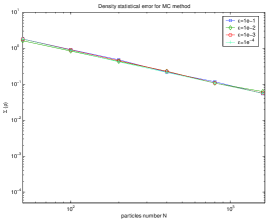
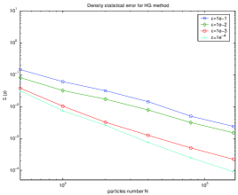
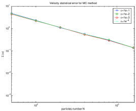
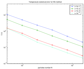
Figure 1: Statistical error test: Solution at $t=0.05$ for density (top), velocity (middle) and temperature (bottom). MC method (left), Hydro Guided MC method (right). Knudsen number vary from $\varepsilon=10^{-1}$ to $\varepsilon=10^{-4}$. Squares indicate errors for $\varepsilon=10^{-1}$, diamonds for $\varepsilon=10^{-2}$, circles for $\varepsilon=10^{-3}$ while crosses indicate errors for $\varepsilon=10^{-4}$.

Unsteady shock test

Next we consider an unsteady shock test case. This choice reflects the fact that the method is specifically aimed at situations in which the classical variance reduction technique using time averaging cannot be used or turns out to be useless, since time-averaging or using more particles leads to the same computational effort.

Figures 2 to 5 consider the same initial data for the density, mean velocity and temperature with different initial Knudsen number values, ranging from $\varepsilon=10^{-4}$ to $\varepsilon=10^{-1}$. $100$ particles per cell are used and solutions are averaged over two different realizations. Each Figure depicts the density, mean velocity and temperature from top to bottom, with the pure Monte Carlo solver (on the left) and Moment Guided method (on the right). In addition, we represent solutions of the compressible Euler equations and as reference solution we used a discrete velocity model for the BGK equation [17]. These Figures show a large reduction of fluctuations especially for small Knudsen numbers.

Sod shock tube

Finally we look at the classical Sod Shock Tube test. For this test case, we consider the possibility of using second order fluid solvers. We observe that this choice has the effect of increasing fluctuations far from thermodynamical equilibrium. This is natural since we miss the smoothing effect of a first order scheme. However solutions obtained with first order schemes can be unsatisfactory in some situations because of their large numerical diffusion especially close to thermodynamical equilibrium. The solution which is adopted here consists in switching from the first order to the second order scheme according to the ratio of the thermodynamical flux with respect to the non equilibrium flux. In practice, in each cell, the scheme automatically uses a second order MUSCL scheme when the kinetic term is small and a first order scheme otherwise.

Figures 6 to 9 consider the same initial data for the density, mean velocity and temperature with different initial Knudsen number values, which range from $\varepsilon=10^{-4}$ to $\varepsilon=10^{-1}$. $100$ per cell are used and only one realization is considered. As for the unsteady shock test each figure depicts the density, mean velocity and temperature from top to bottom, with the pure Monte Carlo solver (left) and the Moment Guided method (right). A reference solution obtained through a discrete velocity scheme [17] is represented in each figure as well as the solution of the compressible Euler equations. The figures shows good results for all ranges of Knudsen numbers in terms of reduction of fluctuations. The high order solver does not seem to increase the variance but improves the solution in the fluid limit.

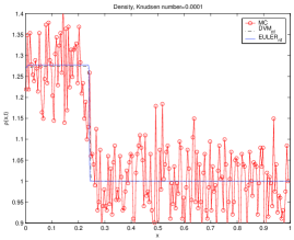
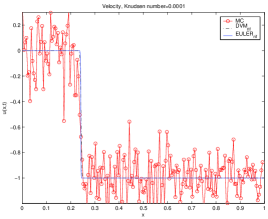
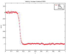
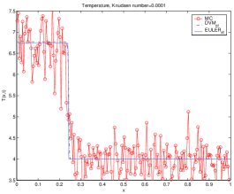
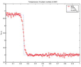
Figure 2: Unsteady Shock: Solution at $t=0.065$ for the density (top), velocity (middle) and temperature (bottom). MC method (left), Moment Guided method MG (right). Knudsen number $\varepsilon=10^{-4}$. Reference solution: dash dotted line. Euler solution: continuous line. Monte Carlo or Moment Guided: circles plus continuous line.

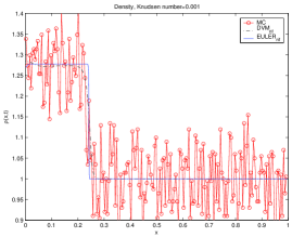
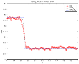
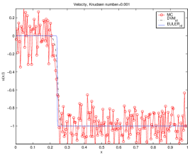
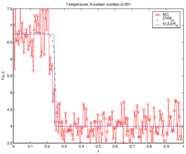
Figure 3: Unsteady Shock: Solution at $t=0.065$ for the density (top), velocity (middle) and temperature (bottom). MC method (left), Moment Guided method MG (right). Knudsen number $\varepsilon=10^{-3}$. Reference solution: dash dotted line. Euler solution: continuous line. Monte Carlo or Moment Guided: circles plus continuous line.

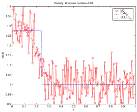
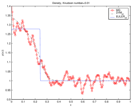
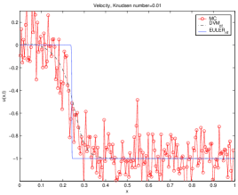
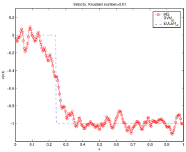
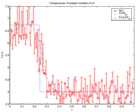
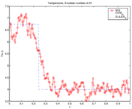
Figure 4: Unsteady Shock: Solution at $t=0.065$ for the density (top), velocity (middle) and temperature (bottom). MC method (left), Moment Guided method MG (right). Knudsen number $\varepsilon=10^{-2}$. Reference solution: dash dotted line. Euler solution: continuous line. Monte Carlo or Moment Guided: circles plus continuous line.

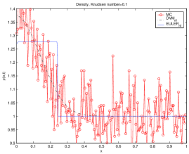
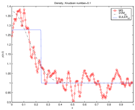
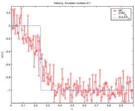
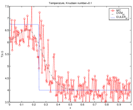
Figure 5: Unsteady Shock: Solution at $t=0.065$ for the density (top), velocity (middle) and temperature (bottom). MC method (left), Moment Guided method MG (right). Knudsen number $\varepsilon=10^{-1}$. Reference solution: dash dotted line. Euler solution: continuous line. Monte Carlo or Moment Guided: circles plus continuous line.

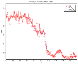
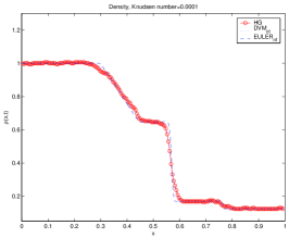
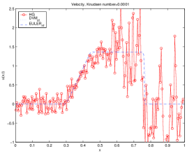
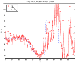
Figure 6: Sod Shock Tube Test: Solution at $t=0.05$ for the density (top), velocity (middle) and temperature (bottom). MC method (left), Moment Guided MG method (right). Knudsen number $\varepsilon=10^{-4}$. Reference solution: dash dotted line. Euler solution: continuous line. Monte Carlo or Moment Guided: circles plus continuous line.

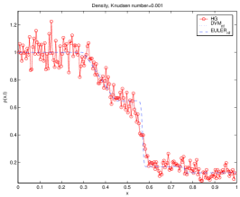
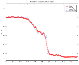
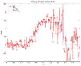
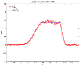
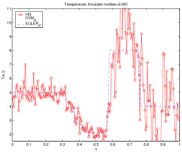
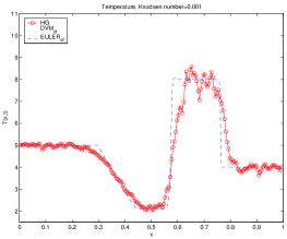
Figure 7: Sod Shock Tube Test: Solution at $t=0.05$ for the density (top), velocity (middle) and temperature (bottom). MC method (left), Moment Guided MG method (right). Knudsen number $\varepsilon=10^{-3}$. Reference solution: dash dotted line. Euler solution: continuous line. Monte Carlo or Moment Guided: circles plus continuous line.

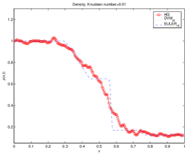
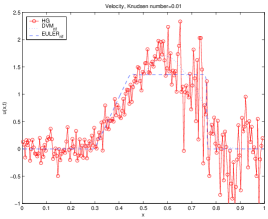
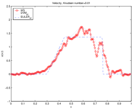
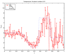
Figure 8: Sod Shock Tube Test: Solution at $t=0.05$ for the density (top), velocity (middle) and temperature (bottom). MC method (left), Moment Guided MG method (right). Knudsen number $\varepsilon=10^{-2}$. Reference solution: dash dotted line. Euler solution: continuous line. Monte Carlo or Moment Guided: circles plus continuous line.

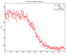
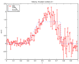
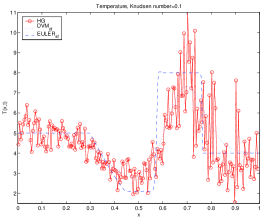
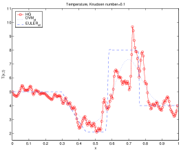
Figure 9: Sod Shock Tube Test: Solution at $t=0.05$ for the density (top), velocity (middle) and temperature (bottom). MC method (left), Moment Guided MG method (right). Knudsen number $\varepsilon=10^{-1}$. Reference solution: dash dotted line. Euler solution: continuous line. Monte Carlo or Moment Guided: circles plus continuous line.

5 Conclusions

We have developed a new class of hybrid methods which aim at reducing the variance in Monte Carlo schemes. The key idea consists in driving particle positions and velocities in such a way that moments given by the solution of the kinetic equation exactly match moments given by the solution of an appropriate set of moment equations. It is important to point out that the schemes which can be derived through this technique can be easily implemented in existing Monte Carlo codes through few modifications: adding a fluid solver and a routine for the moment matching.

Preliminary numerical results show reductions of fluctuations in all regimes compared to DSMC. The reduction becomes stronger as we approach equilibrium. Numerical convergence tests show better performances of the proposed method, in terms of stochastic error, compared to pure Monte Carlo schemes. For these problems the moment guided method seems very promising, leading to solutions which contain less fluctuations at a computational cost which is comparable to the cost of a traditional Monte Carlo solver, and the addition of the cost of a macroscopic solver for the compressible Euler equations, which is usually computationally less expensive than the Monte Carlo method.

Currently, we are working on extensions of the present method to the full Boltzmann equation in the multidimensional case. To this aim we plan to use both classical Monte Carlo methods like Bird or Nanbu methods [18] and time relaxed Monte Carlo (TRMC) techniques [20]. Moreover we plan to explore other possible algorithms which can possibly further reduce fluctuations, such as matching higher order moments and/or using higher order closure of the hierarchy in order to solve a larger set of hydrodynamics equations, or using hybrid representations of the distribution function [5]. We hope to be able to present other results supporting this methodology in the near future [7].

References

- [1] G.A.Bird, Molecular gas dynamics and direct simulation of gas flows, Clarendon Press, Oxford (1994).
- [2] C.K. Birsdall, A.B. Langdon, Plasma Physics Via Computer Simulation, Institute of Physics (IOP), Series in Plasma Physics (2004).
- [3] J. Burt, I. Boyd, A low diffusion particle method for simulating compressible inviscid flows, Journal of Computational Physics, Volume 227, Issue 9, 20 April 2008, pp. 4653-4670
- [4] R. E. Caflisch, Monte Carlo and Quasi-Monte Carlo Methods, Acta Numerica (1998) pp. 1–49.
- [5] R. E. Caflisch, L. Pareschi, Towards an hybrid method for rarefied gas dynamics, IMA Vol. App. Math., vol. 135 (2004), pp. 57–73.
- [6] C. Cercignani, The Boltzmann Equation and Its Applications, Springer-Verlag, New York, (1988).
- [7] P. Degond, G. Dimarco, L. Pareschi, Moment Guided Monte Carlo Schemes for the Boltzmann equation, Work in Progress 2009.
- [8] P.Degond, J.-G. Liu, L. Mieussens, Macroscopic fluid models with localized kinetic upscaling effects, SIAM MMS, vol. 5 (2006), pp. 940-979.
- [9] G. Dimarco, L. Pareschi, A Fluid Solver Independent Hybrid method for Multiscale Kinetic Equations, SIAM J. Sci. Comput. (Submitted).
- [10] H.Grad, On the kinetic theory of rarefied gases, Commun. Pure Appl. Math. 2, 331 (1949).
- [11] W. E, B. Engquist, The heterogeneous multiscale methods, Comm. Math. Sci., vol. 1 (2003), pp. 87-133.
- [12] T. Homolle, N. Hadjiconstantinou, A low-variance deviational simulation Monte Carlo for the Boltzmann equation. Journal of Computational Physics 226 (2007), pp 2341–2358.
- [13] T. Homolle, N. Hadjiconstantinou, Low-variance deviational simulation Monte Carlo. Physics of Fluids 19 (2007) 041701.
- [14] D. Levermore, Moment closure hierarchies for kinetic theories, Journal of Statistical Physics, Vol. 83, No. 5-6, (1996).
- [15] R. J. LeVeque, Numerical Methods for Conservation Laws, Lectures in Mathematics, Birkhauser Verlag, Basel (1992).
- [16] S. Liu, Monte Carlo strategies in scientific computing, Springer, (2004).
- [17] L. Mieussens, Discrete Velocity Model and Implicit Scheme for the BGK Equation of Rarefied Gas Dynamic ,Mathematical Models and Methods in Applied Sciences, Vol. 10 No. 8 (2000), 1121–1149.
- [18] K. Nanbu, Direct simulation scheme derived from the Boltzmann equation, J. Phys. Soc. Japan, vol. 49 (1980), pp. 2042–2049.
- [19] I. Müller, T. Ruggeri, Rational Extended Thermodynamics. Springer Tracts in Natural Philosophy Vol. 37 pp. 393, II Edition - Springer Verlag (1998).
- [20] L. Pareschi, G. Russo, Time Relaxed Monte Carlo methods for the Boltzmann equation, SIAM J. Sci. Comput. 23 (2001), pp. 1253–1273.
- [21] L. Pareschi, Hybrid multiscale methods for hyperbolic and kinetic problems, Esaim Proceedings, Vol. 15, T. Goudon, E. Sonnendrucker & D. Talay Editors, pp.87-120, (2005).
- [22] D. I. Pullin, Direct simulation methods for compressible inviscid ideal gas flow, J. Comput. Phys., 34 (1980), pp. 231–244.