STRUCTURE AND POPULATION OF THE ANDROMEDA STELLAR HALO FROM A SUBARU/SUPRIME-CAM SURVEY

Abstract

We present a photometric survey of the stellar halo of the nearest giant spiral galaxy, Andromeda (M31), using Suprime-Cam on the Subaru Telescope. A detailed analysis of $VI$ color-magnitude diagrams of the resolved stellar population is used to measure properties such as line-of-sight distance, surface brightness, metallicity, and age, and these are used to isolate and characterize different components of the M31 halo: (1) the giant southern stream (GSS), (2) several other substructures, and (3) the smooth halo. First, the GSS is characterized by a broad red giant branch (RGB) and a metal-rich/intermediate-age red clump (RC). The $I$-magnitude of the well-defined tip of the RGB suggests the distance to the observed GSS field of $(m-M)_{0}=24.73\pm 0.11$ ($883\pm 45$ kpc) at a projected radius of $R\sim 30$ kpc from M31’s center. The GSS shows a high metallicity peaked at [Fe/H]$\hskip 3.00003pt\raisebox{1.72218pt}{$>$}\raisebox{-3.01385pt}{$\sim$}\hskip 3.00003pt-0.5$ with a mean (median) of $-0.7$ ($-0.6$), estimated via comparison with theoretical isochrones. Combined with the luminosity of the RC, we estimate the mean age of its stellar population to be $\sim 8$ Gyr. The mass of its progenitor galaxy is likely in the range of $10^{7}$ to $10^{9}M_{\sun}$. Second, we study M31’s halo substructure along the north-west/south-east minor axis out to $R\sim 100$ kpc and the south-west major axis region at $R\sim 60$ kpc. We confirm two substructures in the south-east halo reported by Ibata et al. (2007) and discover two overdense substructures in the north-west halo. We investigate the properties of these four substructures as well as other structures including the western shelf and find that differences in stellar populations among these systems, thereby suggesting each has a different origin. Our statistical analysis implies that the M31 halo as a whole may contain at least 16 substructures, each with a different origin, so its outer halo has experienced at least this many accretion events involving dwarf satellites with mass $10^{7}$–$10^{9}M_{\sun}$ since a redshift of $z\sim 1$. Third, we investigate the properties of an underlying, smooth and extended halo component out to $R>100$ kpc. We find that the surface density of this smooth halo can be fitted to a Hernquist model of scale radius $\sim 17$ kpc or a power-law profile with $\propto R^{-2.17\pm 0.15}$. In contrast to the relative smoothness of the halo density profile, its metallicity distribution appears to be spatially non-uniform with non-monotonic variations with radius, suggesting that the halo population has not had sufficient time to dynamically homogenize the accreted populations. Further implications for the formation of the M31 halo are discussed.

1. Introduction

The advent of large ground-based telescopes and the Hubble Space Telescope (HST) has made it possible to resolve faint individual stars in nearby galaxies, thereby enabling us to study galactic archaeology for such external galaxies in the same way that one studies our home galaxy, the Milky Way. In particular, our knowledge of the stellar halo of the Andromeda galaxy (M31) has dramatically expanded over the last two decades. Indeed, M31 provides us with a global yet detailed view of a galaxy with a similar morphology to the Milky Way.

The most significant discovery in the M31 halo is probably its complex substructures such as the giant southern stream (GSS) in the outer halo (Ibata et al., 2001; Ferguson et al., 2002). This Andromeda GSS has attracted particular attention, as it reveals an on-going hierarchical formation process of M31 and thus places invaluable constraints on galaxy formation models. The GSS contains a high concentration of metal-rich stars (Ibata et al., 2001; Guhathakurta et al., 2006) and is located behind M31 with a significant degree of elongation along the line of sight (McConnachie et al., 2003). Ferguson et al. (2002) discovered significant substructures around M31 by mapping red giant branch (RGB) stars with the Isaac Newton Telescope.

The GSS was once thought to be tidal debris dispersed by interactions with M32 or NGC 205 as judged from its projected trajectory on the sky (Ferguson et al., 2002; Choi et al., 2002), but subsequent studies have revealed that it is probably not related to these two satellites (e.g., Ibata et al., 2004; McConnachie et al., 2004; Guhathakurta et al., 2006; Kalirai et al., 2006a). In particular, spectroscopic observations of GSS stars with Keck/DEIMOS revealed that they show a markedly different radial motion from M32 and NGC 205. Recently, $N$-body numerical simulations have been performed in view of these kinematic results and these have showed that the GSS’s progenitor had a highly eccentric orbit and a mass of about $10^{8}--10^{9}$ M_☉ (Font et al., 2006a; Fardal et al., 2006, 2007). Furthermore, deep photometric observations with HST/ACS reaching down to below the main-sequence turn-off (Brown et al., 2006a, b) detected intermediate-age stars in a GSS field located at a projected distance of $R=20$ kpc from the M31 center as well as in the general halo field at $R=11$ kpc along the southern minor axis (Brown et al., 2003).

In spite of these detailed studies however, it remains unclear what the detailed properties of the GSS’s progenitor galaxy are. Besides, we do not fully understand the connection between the GSS and the other substructures in the M31 halo such as the NE- and W-shelves, although the latest simulations (Fardal et al., 2008; Mori & Rich, 2008) imply a connection among them. To unveil the origin of the GSS, it is of particular importance to carry out the detailed analysis of its stellar populations by assembling a statistically significant set of observational data such as color, metallicity, and age distributions of the stars, in addition to the other halo fields (e.g., Bellazzini et al., 2003). Stellar halos generally have such low surface brightness (SB) that detecting them beyond the Milky Way is a major challenge. For example, Morrison (1993) estimate the SB of the Galactic halo at the solar radius to be $\mu_{V}\sim 27.7$ mag arcsec^-2. The M31 halo was long believed to be an outward extension of its bulge, since surprisingly metal-rich stars ($\rm\langle[M/H]\rangle\sim-0.6$) were found in the inner halo of M31 (e.g., Mould & Kristian, 1986; Couture et al., 1995; Holland et al., 1996; Reitzel et al., 1998). Furthermore, the SB profile measured along the south-east minor axis from integrated light and resolved star counts follows a de Vaucouleurs $R^{1/4}$ profile out to $R=20$ kpc (Pritchet & van den Bergh, 1994), quite unlike the power-law behavior deduced for the halo of the Milky Way. Both the de Vaucouleurs profile and high metallicity are suggestive of an active merger history for the halo (or bulge) component of M31.

The existence of metal-rich populations in the M31 halo has been confirmed by several subsequent studies. Durrell et al. (2001) found that a high-metallicity population with ${\rm[M/H]}\sim-0.5$ is dominated in a field located at $R=20$ kpc along the south-east minor axis, based on a wide-field mosaic CCD camera on CFHT. They also discovered that 30%–40% of the stars at this location belong to a metal-poor population. Furthermore, in their later complementary paper (Durrell et al., 2004), they showed that a similar high-metallicity population is distributed in a field at $R=30$ kpc along the south-east minor axis. Therefore, they concluded that the outer halo shows little or no radial metallicity gradient.

HST has made great contributions to the exploration of the inner halo populations of M31. Using HST/WFPC2 Bellazzini et al. (2003) analyzed the data for 16 fields at different distances from the M31 center, from $R\sim 4.5$ to 35 kpc, down to limiting $V$ and $I$ magnitudes of $\sim 27$. From the metallicity distributions in each field, obtained by comparison of the RGB stars with Galactic globular cluster templates, they detected similar abundance distributions peaked at ${\rm[Fe/H]}\sim-0.6$ in all of the sampled fields. Although in some fields a very metal-rich (${\rm[Fe/H]}\geq-0.2$) component is clearly present, possibly attributable to disrupted disk populations, they identified no evident metallicity gradient in their limited region. Ferguson et al. (2005) and Richardson et al. (2008) investigated M31 inner substructures discovered by Ferguson et al. (2002), based on the deep HST/ACS survey spanning the range from $R\sim 11.5$ to 45 kpc reaching a few magnitudes below the RC. Their systematic surveys confirmed that the inner halo of M31 is strongly polluted by metal-rich and intermediate-age populations disrupted from the M31 disk and the GSS by interactions between M31 and dwarf galaxies.

Brown et al.’s studies based on ultra-deep HST/ACS observations have unraveled star-formation histories in selected locations of the M31 halo (Brown et al., 2003, 2004, 2006a, 2006b, 2007, 2008). With a minimum of 32 orbits per field, these observations have been sufficiently deep to resolve stars below the oldest main-sequence turn-off. Brown et al. (2003) first demonstrated that a minor axis field projected at $R=11$ kpc contains an indisputable population in age (predominantly 6–10 Gyr) and abundance (${\rm[Fe/H]}>-0.5$). Brown et al. (2006b) present results from inner halo fields they associate with the “tidal stream,” “outer disk,” and “spheroid”. In all cases, the fields were shown to have experienced an extended star-formation history, in contrast, they quantified differences between them. Brown et al. (2007) investigated a field at 21 kpc and found evidence that its population is marginally older and more metal poor than the inner halo field. Furthermore, Brown et al. (2008), based on an additional field at $R=35$ kpc, found that the mean ages (the mean [Fe/H] values) at 11, 21 and 35 kpc gradually change like 9.7 ($-0.65$), 11.0 ($-0.87$) and 10.5 ($-0.98$) Gyr (dex), respectively.

The inclusion of kinematic information has been extremely useful but has also added another dimension of complexity to the puzzle. Spectroscopic studies of Guhathakurta et al. (2005) uncovered successfully the presence of an extended halo component having a power-law SB profile of $R^{-2.3}$ over the range $R=30$–165 kpc resembling the Milky Way’s halo, while the SB of M31’s spheroid at $R<30$ kpc has been known to show an $R^{1/4}$ law resembling a galactic bulge (Pritchet & van den Bergh, 1994; Durrell et al., 2004; Irwin et al., 2005; Gilbert et al., 2006). They also reported that M31’s halo may extend to $R\gtrsim 165$ kpc, suggesting that halo stars of M31 and the Milky Way occupy a substantial volume fraction of our Local Group. However, it remains to be seen whether this flat portion of the halo profile is affected by substructure.

In the meantime Reitzel & Guhathakurta (2002) analyzed a sample of 29 stars in a field at $R=19$ kpc on the minor axis and found the mean metallicity to be in the range of ${\rm[Fe/H]}=-1.9$ to $-1.1$. Despite still remaining uncertainties of calibration and sample selection issues, their estimated mean metallicity is significantly lower than the results deduced from the above photometric analyses. Kalirai et al. (2006b) and Chapman et al. (2006) recently discovered a metal-poor halo out to $R=165$ kpc that is similar to that of the Galaxy, both in terms of its metallicity, radial profile, as well as the amount of substructure.

As noted above, the stellar halo of M31 as well as the Milky Way is filled with quite complex fossil records. Our principal goal is thus to identify each component of the halo and clarify its formation history. To do so, we need to obtain both the global and local structures in the stellar halo and deduce plausible origins of them. Detailed studies based on large numbers of stars, such as with wide-field imagers, are required to investigate the fundamental nature of the large halo regions in M31. Indeed, our external viewpoint for this galaxy makes it possible to study the entire area of its halo (Ibata et al., 2007); detailed stellar maps will allow us to detect giant streams as well as a wealth of fainter substructures at SB levels of $\sim 30$ mag arcsec^-2. In the south-quadrant halo of M31, Ibata et al. also discovered much fainter stream-like substructures reaching $\sim 34$ mag arcsec^-2 as well as previously unknown surviving dwarf satellites and peculiarly extending outer globular clusters. The properties of these faint substructures in the outer halo, such as radial distributions of surface brightness and metallicity, have been reproduced by some recent numerical simulations (e.g., Bullock & Johnston, 2005; Abadi et al., 2006; Johnston et al., 2008), which thus provide us with useful theoretical templates to understand the formation history of the stellar halo.

Here we report on our wide-field, photometric observations of the M31 halo, using Subaru/Suprime-Cam, aimed at obtaining the detailed physical properties of the M31 halo, such as color-magnitude diagrams (CMDs), metallicity distributions, surface brightness and age, compared with previous studies using CFHT/MegaCam (e.g., Ibata et al., 2007). Our Suprime-Cam survey is deeper and covers as-yet unexplored fields along the north-west minor axis of the halo as well as some fields in the south-quadrant halo already explored by other telescopes. A large set of our imaging data provides an important clue to understanding the complex halo substructures and their origin in the course of the formation history of the M31 halo.

The layout of this paper is as follows. In § 2, we present observations and detailed procedure for calibrating the photometric Suprime-Cam data. § 3 is devoted to our results for the quantitative analysis of the GSS, including the morphology of the obtained CMDs, the distance estimate using the tip of the RGB stars (TRGB), their metallicity distribution using the observable globular cluster templates and theoretical isochrones, and their age distribution based on the luminosity distribution of the stars. In § 4, we expand our method to the entire regions of the M31 halo in order to globally determine the fundamental properties of the M31 halo. Then, we elaborate the technique for separating the foreground and background contaminants. The spatial distributions of the stellar populations in the M31 halo are also presented in the section. Furthermore, we present the CMDs of the detected streams and other spatial substructures, and show the radial profiles and the radial metallicity distributions of the stellar populations in the halo. Finally, we discuss the implications of our results and compare with previous studies. In § 8 we draw conclusions and future directions.

Throughout this work we adopt the M31 Cepheid distance modulus of $(m-M)_{0}=24.43\pm 0.06$ ($\sim$ 770 kpc) from Freedman & Madore (1990), if not otherwise specified. Reddening corrections are applied in each field based on the extinction maps of Schlegel et al. (1998), and the Dean et al. (1978) reddening law $E(V-I)=1.34E(B-V)$ and $A_{I}=1.31E(V-I)$. We also adopt the convention that $R$ and $r$ denote, respectively, the projected radius and three-dimensional radius from the M31 center.

2. Data

2.1. Suprime-Cam Observations

In our observational studies of Andromeda’s stellar halo, we use the Suprime-Cam imager (Miyazaki et al., 2002) on the 8.2-m Subaru Telescope (Iye et al., 2004) on Mauna Kea in Hawaii. Suprime-Cam consists of ten $2045\times 4070$ CCDs with a scale of $0\farcs 202$ per pixel and covers a total field-of-view $34\arcmin\times 27\arcmin$. Using this wide-field imager, we have carried out a systematic imaging survey of two series of fields far from the M31 center: fields along the minor and major axis of the spheroid (hereafter referred to as “halo” fields) and fields along the Andromeda GSS (“stream” fields). Our targeted fields of the halo and stream fields are, respectively, located at between 22 and 91 kpc (Figure 1) and at $\sim$ 32 kpc ($2\fdg 4$) from the M31 center. Tables 1 summarizes the names of these targeted fields and their observations.

During four nights in August 2004, we obtained the Suprime-Cam image of the one stream field (hereafter referred to as GSS1) and also made imaging surveys for eleven halo fields in the south part of M31 (SE1–9 and SW1–2). In addition to these targeted fields, we obtained the imaging data at the control field (hereafter referred to as CompL103Bm21) to estimate the number of foreground dwarf stars of the Milky Way and unresolved background galaxies in each M31’s field. The weather conditions in August 2004 were unfortunately slightly poor, with seeing varying from $0\farcs 7-1\farcs 5$. Therefore, we carried out additional imaging of GSS1, SE1, SE6, SE9 and SW1 on a photometric night in August 2005 in order to calibrate the data. In August 2007 and August 2008, the halo fields in the north part of M31 (NW1–15) were observed in photometric conditions, along with the control fields (CompL103Bm25 and CompL103Bm16_5).

The observations were made with Johnson $V$-band and Cousins $I$-band filters. Typical exposure times of each object field observed in 2004–2005 and 2007 are 1800 sec and 720 sec in $V$ and $I$ band, respectively, and those in 2008 are 1440 and 2160 sec in $V$ and $I$ band, respectively, so that the images reach down to magnitude of the RC of M31. Each field was observed with adequate dithering pattern to cover gaps between adjacent CCD chips. Some of these fields were observed in short exposures of 5 and 10 s (12 and 15 s) in $V$ ($I_{c}$) bands. They are used to improve photometric accuracy and to investigate space variation of foreground dwarf stars along the galactic latitude at the same galactic longitude. In addition, all the targeted fields in the M31 halo are overlapping with neighboring fields in order to calibrate the adjacent fields whose photometric zero points are unknown in poor condition, such as SE2, SE3 and so on.

The position angle of each field observed in 2004–2005 is 0°, i.e., North is up and East is to the left of each image. In the 2007–2008 runs, the position angle of each field is 38°, i.e., the longer side of each image is aligned to the minor axis of M31 in order to obtain many pointings along the far outer part of M31’s halo. For more details, see Table 1.

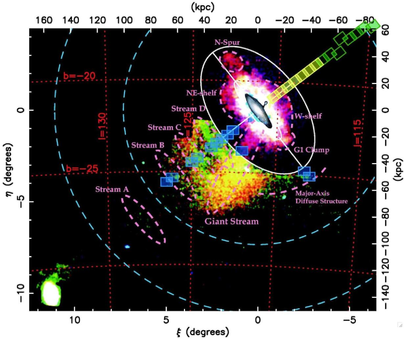
Figure 1.— Locations of our Subaru/Suprime-Cam fields (rectangular areas), overlaid on the color-composited stellar density map [taken from Figure 53 of the Ibata et al. (2007) paper], in which red, green, and blue colors show, respectively stars with $-0.7<{\rm[Fe/H]}<0.0$, $-1.7<{\rm[Fe/H]}<-0.7$ and $-3.0<{\rm[Fe/H]}<-1.7$. Our Suprime-Cam fields characterized by blue, yellow, and green rectangles were obtained in 2004, 2007 and 2008, respectively. Table 1 presents a log of these observations.

Table 1Observational status for target fields

Field	Coordinates	Date	Filter	Exposure	Airmass	Seeing	50% completeness
$R_{\rm proj}$	$(\alpha_{2000}/\delta_{2000})$	mm/yyyy		(sec)		(mag)
GSS1	$00^{\rm h}47^{\rm m}38\fs 11$	08/2004	$V$	$600\times 5$	1.7	$1\farcs 07$	25.95
($\approx 32$ kpc)	$+39{\arcdeg}05{\arcmin}57{\farcs}4$	08/2004	$I$	$300\times 6$	1.2	$0\farcs 92$	25.00
SE1	$00^{\rm h}50^{\rm m}09\fs 16$	08/2004	$V$	$600\times 3$	1.3	$1\farcs 00$	26.40
($\approx 24$ kpc)	$+40{\arcdeg}08{\arcmin}36{\farcs}4$	08/2004	$I$	$300\times 6$	1.1	$0\farcs 71$	25.66
SE2	$00^{\rm h}51^{\rm m}38\fs 06$	08/2004	$V$	$600\times 5$	1.2	$1\farcs 13$	26.34
($\approx 29$ kpc)	$+39{\arcdeg}55{\arcmin}03{\farcs}4$	08/2004	$I$	$300\times 6$	1.1	$0\farcs 93$	25.24
SE3	$00^{\rm h}53^{\rm m}06\fs 96$	08/2004	$V$	$600\times 3$	1.4	$1\farcs 03$	26.30
($\approx 34$ kpc)	$+39{\arcdeg}41{\arcmin}30{\farcs}4$	08/2004	$I$	$300\times 6$	1.1	$0\farcs 82$	25.40
SE4	$00^{\rm h}54^{\rm m}35\fs 86$	08/2004	$V$	$600\times 5$	1.3	$1\farcs 13$	26.34
($\approx 39$ kpc)	$+39{\arcdeg}27{\arcmin}57{\farcs}4$	08/2004	$I$	$300\times 6$	1.1	$0\farcs 87$	25.27
SE5	$00^{\rm h}56^{\rm m}04\fs 76$	08/2004	$V$	$600\times 5$	1.5	$1\farcs 21$	26.24
($\approx 44$ kpc)	$+39{\arcdeg}14{\arcmin}24{\farcs}4$	08/2004	$I$	$300\times 6$	1.1	$0\farcs 99$	25.03
SE6	$01^{\rm h}00^{\rm m}04\fs 68$	08/2004	$V$	$600\times 2$	1.6	$1\farcs 05$	26.12
($\approx 55$ kpc)	$+38{\arcdeg}54{\arcmin}58{\farcs}5$	08/2004	$I$	$300\times 6$	1.1	$1\farcs 00$	25.37
SE7	$01^{\rm h}01^{\rm m}31\fs 73$	08/2004	$V$	$600\times 2$	1.4	$1\farcs 01$	26.12
($\approx 60$ kpc)	$+38{\arcdeg}41{\arcmin}25{\farcs}5$	08/2004	$I$	$300\times 5$	1.1	$0\farcs 89$	25.09
SE8	$01^{\rm h}09^{\rm m}04\fs 58$	08/2004	$V$	$600\times 3$	1.4	$0\farcs 94$	26.48
($\approx 84$ kpc)	$+37{\arcdeg}37{\arcmin}39{\farcs}5$	08/2004	$I$	$300\times 6$	1.1	$0\farcs 74$	25.77
SE9	$01^{\rm h}10^{\rm m}30\fs 09$	08/2004	$V$	$600\times 3$	1.2	$1\farcs 00$	26.47
($\approx 89$ kpc)	$+37{\arcdeg}24{\arcmin}06{\farcs}5$	08/2004	$I$	$300\times 6$	1.1	$0\farcs 71$	25.77
SW1	$00^{\rm h}29^{\rm m}16\fs 28$	08/2004	$V$	$600\times 3$	1.6	$1\farcs 08$	26.31
($\approx 58$ kpc)	$+37{\arcdeg}49{\arcmin}40{\farcs}4$	08/2004	$I$	$300\times 6$	1.1	$0\farcs 75$	25.58
SW2	$00^{\rm h}28^{\rm m}12\fs 40$	08/2004	$V$	$600\times 3$	1.6	$0\farcs 98$	26.42
($\approx 63$ kpc)	$+37{\arcdeg}33{\arcmin}23{\farcs}4$	12/2005	$I$	$300\times 7$	1.1	$0\farcs 98$	25.23
NW1	$00^{\rm h}38^{\rm m}07\fs 50$	08/2007	$V$	$240\times 3$	1.4	$0\farcs 65$	25.99
($\approx 15$ kpc)	$+41{\arcdeg}56{\arcmin}47{\farcs}0$	08/2007	$I$	$180\times 4$	1.3	$0\farcs 67$	24.95
NW2	$00^{\rm h}36^{\rm m}12\fs 20$	08/2007	$V$	$240\times 3$	1.1	$0\farcs 69$	26.18
($\approx 21$ kpc)	$+42{\arcdeg}13{\arcmin}31{\farcs}8$	08/2007	$I$	$180\times 4$	1.1	$0\farcs 65$	25.35
NW3	$00^{\rm h}34^{\rm m}16\fs 90$	08/2007	$V$	$240\times 3$	1.1	$0\farcs 69$	26.34
($\approx 27$ kpc)	$+42{\arcdeg}30{\arcmin}16{\farcs}6$	08/2007	$I$	$180\times 4$	1.2	$0\farcs 59$	25.87
NW4	$00^{\rm h}32^{\rm m}21\fs 60$	08/2007	$V$	$240\times 3$	1.1	$0\farcs 63$	26.74
($\approx 33$ kpc)	$+42{\arcdeg}47{\arcmin}01{\farcs}4$	08/2007	$I$	$180\times 4$	1.1	$0\farcs 61$	25.74
NW5	$00^{\rm h}30^{\rm m}26\fs 30$	08/2007	$V$	$240\times 3$	1.1	$0\farcs 61$	26.72
($\approx 39$ kpc)	$+43{\arcdeg}03{\arcmin}46{\farcs}2$	08/2007	$I$	$180\times 4$	1.1	$0\farcs 61$	25.74
NW6	$00^{\rm h}28^{\rm m}31\fs 00$	08/2007	$V$	$240\times 3$	1.1	$0\farcs 59$	26.63
($\approx 45$ kpc)	$+43{\arcdeg}20{\arcmin}31{\farcs}0$	08/2007	$I$	$180\times 4$	1.1	$0\farcs 65$	25.60
NW7	$00^{\rm h}26^{\rm m}35\fs 70$	08/2007	$V$	$240\times 3$	1.3	$0\farcs 65$	26.46
($\approx 51$ kpc)	$+43{\arcdeg}37{\arcmin}15{\farcs}8$	08/2007	$I$	$180\times 4$	1.2	$0\farcs 57$	25.93
NW8	$00^{\rm h}24^{\rm m}25\fs 10$	08/2008	$V$	$240\times 5$	1.1	$1\farcs 07$	25.70
($\approx 57$ kpc)	$+43{\arcdeg}52{\arcmin}56{\farcs}5$	08/2008	$I$	$360\times 6$	1.1	$0\farcs 87$	25.16
NW9	$00^{\rm h}22^{\rm m}26\fs 10$	08/2008	$V$	$240\times 5$	1.1	$1\farcs 07$	25.72
($\approx 63$ kpc)	$+44{\arcdeg}09{\arcmin}41{\farcs}3$	08/2008	$I$	$360\times 6$	1.1	$0\farcs 89$	25.02
NW10	$00^{\rm h}19^{\rm m}58\fs 60$	08/2008	$V$	$240\times 8$	1.1	$1\farcs 05$	25.94
($\approx 70$ kpc)	$+44{\arcdeg}20{\arcmin}03{\farcs}1$	08/2008	$I$	$360\times 6$	1.1	$0\farcs 71$	25.47
NW11	$00^{\rm h}18^{\rm m}23\fs 20$	08/2008	$V$	$240\times 7$	1.1	$0\farcs 99$	25.98
($\approx 78$ kpc)	$+44{\arcdeg}59{\arcmin}02{\farcs}1$	08/2008	$I$	$360\times 6$	1.1	$0\farcs 71$	25.62
NW12	$00^{\rm h}16^{\rm m}30\fs 30$	08/2008	$V$	$240\times 29$	1.2	$0\farcs 71$	27.06
($\approx 82$ kpc)	$+45{\arcdeg}00{\arcmin}59{\farcs}4$	08/2008	$I$	$360\times 18$	1.1	$0\farcs 67$	25.94
NW13	$00^{\rm h}14^{\rm m}29\fs 10$	08/2008	$V$	$240\times 6$	1.2	$0\farcs 63$	26.88
($\approx 88$ kpc)	$+45{\arcdeg}17{\arcmin}44{\farcs}1$	08/2008	$I$	$360\times 6$	1.1	$0\farcs 67$	25.60
NW14	$00^{\rm h}12^{\rm m}27\fs 20$	08/2008	$V$	$240\times 6$	1.2	$0\farcs 67$	26.60
($\approx 94$ kpc)	$+45{\arcdeg}34{\arcmin}28{\farcs}9$	08/2008	$I$	$360\times 6$	1.1	$0\farcs 75$	25.53
NW15	$00^{\rm h}09^{\rm m}46\fs 50$	08/2008	$V$	$240\times 6$	1.1	$0\farcs 75$	26.80
($\approx 100$ kpc)	$+45{\arcdeg}42{\arcmin}43{\farcs}1$	08/2008	$I$	$360\times 6$	1.1	$0\farcs 75$	25.57
CompL103Bm21	$23^{\rm h}17^{\rm m}00\fs 00$	08/2007	$V$	$240\times 3$	1.1	$0\farcs 69$	26.43
$[l=103\arcdeg,b=-21\arcdeg]$	$+38{\arcdeg}32{\arcmin}00{\farcs}0$	08/2007	$I$	$180\times 4$	1.1	$0\farcs 53$	26.13
CompL103Bm25	$23^{\rm h}25^{\rm m}30\fs 00$	08/2008	$V$	$240\times 8$	1.1	$0\farcs 71$	26.53
$[l=103\arcdeg,b=-25\arcdeg]$	$+34{\arcdeg}29{\arcmin}50{\farcs}0$	08/2008	$I$	$360\times 6$	1.0	$0\farcs 67$	25.76
CompL103Bm16_5	$23^{\rm h}06^{\rm m}30\fs 00$	08/2008	$V$	$240\times 22$	1.2	$0\farcs 71$	27.15
$[l=103\arcdeg,b=-16.5\arcdeg]$	$+42{\arcdeg}13{\arcmin}00{\farcs}0$	08/2008	$I$	$360\times 27$	1.1	$0\farcs 71$	26.13

2.2. Reduction and Photometry

The raw data were reduced in the standard procedures, with the software package SDFRED, a useful pipeline developed to optimally deal with Suprime-Cam images (Yagi et al., 2002; Ouchi et al., 2004). Using SDFRED, we obtained a mean-stacked image for each field, which covers $34\arcmin\times 27\arcmin$ field-of-view.

We then conducted PSF-fitting photometry using the IRAF version of the DAOPHOT-II software (Stetson, 1987). We adopted a 3 $\sigma$ detection threshold for the initial object detection/photometry pass and repeated the PSF-fitting photometry twice with 5 $\sigma$ and 7 $\sigma$ detection thresholds, respectively, in order to account for blended stars. A stellar PSF template was constructed from 10–100 bright, not saturated, isolated stellar objects per image. Finally, we merged two independent $V$-band and $I$-band catalogues into a combined catalogue using 2-pixel matching radius. Note that we cannot detect objects near the edge of a field in case of adopting a 1-pixel matching radius.

When conducting photometry, we divide a Suprime-Cam field into a few subfields and photomery is carried out for each subfield separately. For example, for fields with PA$=0\arcdeg$ we divide them to four subfields (labeled by “a”, “b”, “c” and “d”), while for fields with PA$=38\arcdeg$, we divide them to two subfields (one is not labeled and the other is labeled by “d”). If we perform detection and photometry using DAOPHOT without dividing to subfields, stellar-like objects near the edge of field-of-view ($34\arcmin\times 27\arcmin$) are not properly detected because the actual PSF is largely varying depending on the location. Even if we consider the space variation of PSF by means of making a model PSF function to detect objects ($PSF$ task), it results in inducing erratic values of $sharpness$ and $chi$ in some DAOPHOT parameters. Actually, when we have detected objects without dividing one field-of-view, we have failed to detect approximately 20% of stellar samples of M31 red giants and Milky Way dwarf stars identified by Keck/DEIMOS spectroscopic observations (see §2.4.1).

2.3. The Artificial Star Experiments

2.3.1 Completeness

To evaluate incompleteness due to low signal-to-noise ratio and crowding, We have conducted the artificial star experiments as detailed below. We have added a sufficient number of artificial stars to all the original images, where each star has the PSF as determined from many bright stars in each frame in § 2.2, and the range of the magnitudes is $20\leq V,I\leq 28$ with a binning step of 0.2 mag. Note that for a portion of the large images the binning is 0.5 mag in the brighter parts with $V=23$ mag. To prevent these stars from interfering with one another, we have divided the Suprime-Cam frames into grids of cells of $200$ pixels width and have randomly added one artificial star to each cell for each run. In addition, we constrain each artificial star to have 20 pixels from the edges of the cell. We note that a similar procedure to ours has recently been adopted by Piotto & Zoccali (1999) and Bellazzini et al. (2002). In this way we can control the minimum distance between adjacent artificial stars. At each run the absolute position of the grid is randomly changed in a way that, after a large number of experiments, the stars are uniformly distributed in coordinates (see also Tosi et al., 2001).

The stars, which have a Penny2 function expressed as the analytic component of the PSF model computed by the DAOPHOT-II PSF task and are quadratically variable over the image, were added on the original frame including Poisson photon noise. Each star has been added to the $V$ and $I$ coadded frames. For the artificial frames we have performed detection and photometry following the method described in § 2.2 and extracted stellar-like objects by applying our established selection criteria based on DAOPHOT parameters (see § 2.3.2).

About 500 to 4300 stars, were configured for each run, and the total number is about 18,000 to 140,000 in each band image, where the number of added artificial stars depends on the subfield size. After the above-mentioned detection/photometry and selection, the final recovered objects were regarded as stars, if they reside within 2 pixel of the position of the added star and their magnitudes are within 0.75 mag of the assigned values. In this task, the completeness is defined as a number fraction of recovered stars in added stars. In Figure 2, we plot the completeness fractions ($=N_{\rm output}/N_{\rm input}$) as a function of input $V$ (filled circles) and $I$ (open rectangles) magnitudes in the NW3 field as estimated by the current artificial star experiments. Note that the continuous line is not a fit to the data but is simply the line connecting them. Alphabetical letters labeled in each field of the south quadrant area of the M31 halo, such as “a”, “b”, “c” and “d” represent the subfields which are obtained by dividing a single Suprime-Cam field into four subfields. In these subfields, the 25% overlapping regions (labeled by “c” for SE and SW fields and by “d” for GSS fields) indicate slightly deep completeness limits. In contrast, the regions which are overlapping the nearby fields along the North-West minor axis of the M31 halo are labeled by “d”, meaning “deep”. The rightmost column of Table 1 shows the 50% completeness limits of V- and I-band in each subfield. In all the fields the completeness is larger than 80% at $I\leq 24.5$, and our imaging data are much deeper than the previous studies using ground-based telescopes, e.g. McConnachie et al. (2003), Durrell et al. (2001, 2004) and Ibata et al. (2007). The 50% completeness is reached at $V\geq 25.70$ and $I\geq 24.85$ in all the fields.

Figure 2.— Completeness fraction ($=N_{\rm output}/N_{\rm input}$) as a function of input $V$ (filled circles) and $I$ (open rectangles) magnitudes in the NW3 field as estimated by the current artificial star experiments.

2.3.2 Selection of Stellar-Like Objects Based on DAOPHOT Parameters

In extracting stellar-like objects from the catalogs containing all the detected objects, we apply selection criteria based on DAOPHOT parameters such as the $sharpness$, $chi$, and the photometric error, which are simulated in the above artificial star experiments. The $sharpness$ parameter estimates the intrinsic angular size of the measured objects. It is roughly defined as the difference between the square of the width of the object and the square of the width of PSF and has values close to zero for single stars, large positive values for blended doubles and partially resolved galaxies, and large negative values for cosmic rays and blemishes. The $niter$ parameter is the number of iterations the solution required to achieve convergence. The $chi$ parameter assesses the estimated goodness-of-fit. It is the ratio of the observed pixel-to-pixel mean absolute deviation from the profile fit, to the value expected on the basis of the noise as determined from Poisson statistics and the readout noise.

The simulation results of the four parameters to select stellar-like objects are illustrated in Figure 3. The solid and dashed lines show mean value and 4 $\sigma$ deviations of each parameter measured for artificial stars, respectively. We choose as “good” stars those sources lying within two hyperbolic envelopes around the sharpness value of zero (Fig. 3 bottom left panel), that is, within the 4 sigma deviation drawn by the dashed lines, below the 4 sigma lines of the niter value (top right panel) and the chi value (bottom right panel), and to the right of the maximum allowed $\sigma$ error at a given magnitude (top left panel). The remaining cosmic-ray blemishes and resolved background galaxies were then rejected. However, this sigma criterion slightly changes with the sky condition because this simulation is prone to misclassify nearly point-like background galaxies as stellar objects under the worse seeing condition. We have tested the seeing effect by comparing the overlapping region between the NW7 field with good seeing and the NW8 field with bad seeing. To adjust the surface brightness of the NW8 subfield to that of the NW7 subfield, we have found a 1 sigma shift of our adopted selection criteria. Therefore, we apply the 3 sigma criteria for the poor data with the larger seeing size than 0$\farcs$8.

However, this morphological segregation method cannot completely distinguish M31 halo stars from other point sources such as Galactic foreground dwarf stars, and compact extragalactic objects. Thus, we have to remove these contaminations from the targeted fields statistically. To estimate the contaminations, we adopted a control field located at the Galactic latitude comparable to that of our targeted fields, on the assumption that it has almost the same abundance of foreground and background objects as that in the M31 spheroid fields. Actually, we found uniform galaxy distribution in our control fields. As described in § 4.1.1, to further refine our control field, we will consider the finite spatial gradient in the number of foreground disk dwarf stars of the Milky Way along the Galactic latitude.

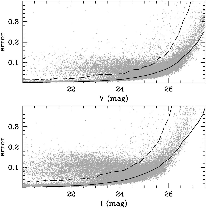
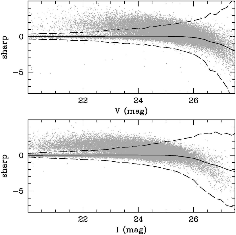
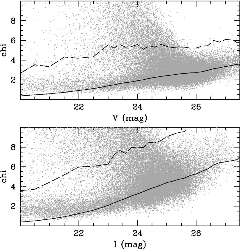
Figure 3.— Photometry selection criteria based on the photometric error, niter, sharpness and chi parameters from DAOPHOT programs are plotted as functions of $V$ and I magnitudes. All of the detected objects after matching up to separate $V$ and I catalogs derived from the observation of NW3 field are illustrated as light gray dots. The solid lines show returned mean values of each simulated parameter, and the dashed lines denote the 4 sigma deviations. We select final objects within the 4 sigma deviations.

2.3.3 Photometric Errors

These artificial star experiments are implemented to ascertain not only the completeness but also more accurate photometric errors in our data. These are quantified as the average of differences between input and output magnitudes of an artificial star at a specific magnitude, shown in Figure 4. The mean magnitude difference $\Delta{\rm mag}={\rm mag}_{\rm input}-{\rm mag}_{\rm output}$ is consistent with 0 for magnitudes brighter than a 80% completeness limit ($V\sim 26$ and $I\sim 25.5$ in case of the NW3 field). The shift toward systematically brighter measured magnitudes, which signals the occurrence of blending of the stellar images, is smaller than 0.09 mag at the magnitude bin corresponding to 50% completeness level. The right panels of Figure 4 show mean error as a function of magnitude as measured from these simulations.

Figure 4.— Typical mean error as a function of magnitude for NW3 field. On the left we plot difference between the measured and input magnitude as a function of input magnitude for all the stars from our completeness simulations, while the panels on the right show mean error as a function of magnitude as measured from these simulations. Only those simulated stars that were recovered within 2 pixels of the input position and that had magnitudes within 0.75 of the input magnitude are considered to be recovered. There is no systematic shift of the mean magnitude difference, and the typical 1 $\sigma$ errors at the 50% completeness magnitude limits are of the order of 0.3 mag.

2.4. Comparison with Published Data

2.4.1 Detection featuring Keck/DEIMOS Spectroscopic Samples

In SE3 field, there are some M31’s RGB stars identified by Gilbert et al. (2006). Using the DEIMOS instrument on the Keck II 10m telescope, their RGB samples have been confirmed based on five criteria: radial velocity, photometry in the intermediate-width DDO51 band to measure the strength of the MgH/Mg$b$ absorption features, strength of the Na${\rm I}~{}\lambda$8190 absorption line doublet, location within an ($V-I,I$) color-magnitude diagram, and comparison of photometric (color-magnitude diagram based) versus spectroscopic (Ca${\rm II}~{}\lambda$8500 triplet based) metallicity estimates. Therefore, to test the validity of our detection method, we match up our photometric catalogs with their spectroscopic catalogs using a 10-pixel matching radius.

Figure 5 shows a small section of the SE3 field ($2250\times 5200$ pixels, the dotted rectangle in Figure 6). This field is located close to the center of the DEIMOS spectroscopic field, at $\alpha_{2000}=00^{\rm h}54^{\rm m}08\fs 34,\delta_{2000}=+39\arcdeg 41\arcmin 51\farcs 7$. The colored circles denote those objects whose spectra are measured by Keck: M31 red giants and Milky Way dwarf stars (red, 61 objects), background galaxies/QSOs (cyan, 31 objects), alignment stars (blue, 6 objects) used to carry out fine astrometric alignment of the DEIMOS multislit mask, spectroscopic failures (yellow, 5 objects) and guide stars (magenta, 2 objects) only used for coarse astrometric alignment - no spectra are obtained for them. In contrast, green X points show our Subaru objects corresponding to all the Keck samples in our final star catalog.

The number of stellar-like objects detected by our Subaru observation is 56 objects, and the number of missing objects is less than 7% of the total. Note that one out of 61 spectroscopic stellar-like objects is in the masked region, and therefore the total number is 60 objects. Figure 7 shows the magnitude difference between these different systems. The 4 missing objects are removed from the final catalog because they have somewhat large $sharpness$ and $chi$ values in their magnitude.

We have also detected 12 objects classified as background galaxies/QSOs by the Keck spectroscopic observation. This is 40% of the total number, and the contaminations attributable to these background objects are moderately removed. This suggests that all the background contaminations are never rejected using only DAOPHOT morphological parameters. Therefore, the remaining background contaminations are removed in comparison to the data of Control Fields located outside M31’s halo (for more details, see § 2.3.2).

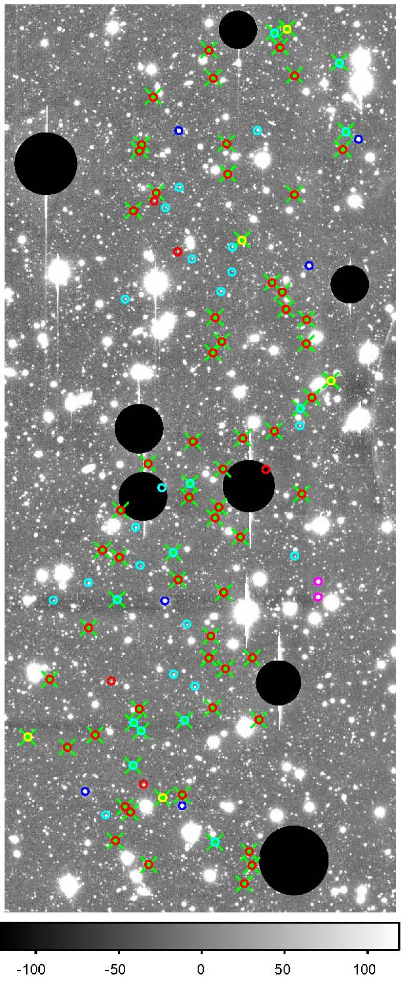
Figure 5.— A small section of the SE3 field. This is a V-band coadded image with the total exposure time of 30 min and covers a field-of-view $7.6\arcmin\times 17.5\arcmin$.

2.4.2 Photometry featuring KPNO 4m Telescope Samples

In this section, we compare our photometric data with other photometric data taken with the Mosaic camera on the Kitt Peak National Observatory (KPNO) 4m telescope in the Washington System $M$ and $T_{2}$. Photometric transformation relations from Majewski et al. (2000) were used to derive Johnson-Cousins $V$ and $I$ magnitudes from the $M$ and $T_{2}$ magnitudes. The color transformation follows:

$$(V-I)=(V-T_{\rm 2})=-0.006+0.008(M-T_{\rm 2}).$$ (1)

With the assumption $I=T_{\rm 2}$ and the above relation, we converted to a $V$ magnitude

$$V=M-0.006-0.200(M-T_{\rm 2}).$$ (2)

Figure 6 shows sky positions observed by three different telescopes, which are used to evaluate the efficiency of our detection/photometry. The “a0” field is associated with our SE1, SE2 and SE3 fields, and the “mask4” field covers our SE3, SE4 and SE5 fields, and the “m6” field overlaps our SE8 and SE9 fields.

We compare the magnitudes based on the Subaru calibration with the magnitudes based on the KPNO calibrations after matching up two different catalogs using a 3-pixel matching radius. We extract stellar-like objects based on the DAOPHOT parameters ($merr<0.02$, $-0.3<sharp<0.3$ and $chi<4$). In Figure 7, we present a comparison of the two independently determined $V$- and $I$- band flux measurements for the three KPNO fields. The fact that the number of faint stars with $V\gtrapprox 23.5$ and $I\gtrapprox 22.5$ decreases with decreasing flux is due to low signal-to-noise in fainter part of the KPNO survey. The individual $V_{\rm Subaru}$ ($I_{\rm Subaru}$) and $V_{\rm KPNO}$ ($I_{\rm KPNO}$) are found to be in good agreement with one another over most of the magnitude range, indicating that there are no systematic variations in our magnitude measurements.

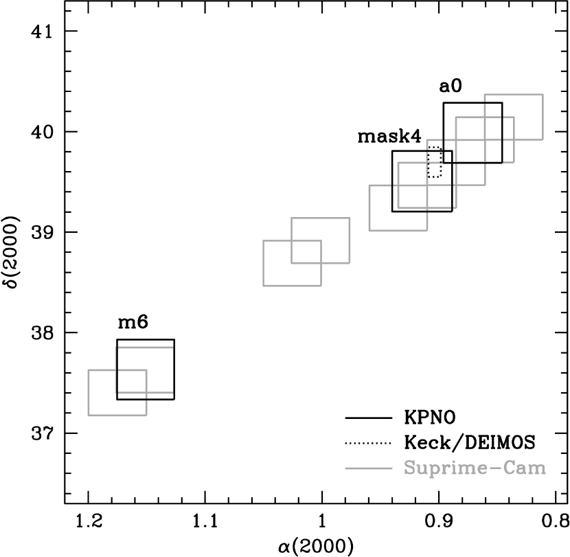
Figure 6.— Sky positions observed by three different telescopes, which they are used to evaluate efficiency of our Detection/Photometry. The gray rectangles represents the position and area of the Subaru/Suprime-Cam image. The solid squares indicate the approximate positions of the KPNO fields. The dotted vertically long rectangle approximates the size and position angle of the DEIMOS spectroscopic slitmask.

Figure 7.— Comparison of Subaru versus KPNO magnitudes of stellar-like objects in the three overlapping regions. For reference, a 1:1 relation is shown as a solid line.

3. The Andromeda Giant Stream

3.1. Morphology of the Color-Magnitude Diagram

Figure 8 shows the CMDs for the GSS (left) and for the control field (right). In this section, we use the SE3 field as the control field. The clearest feature in the stream field is a broad RGB characterized by low-mass, hydrogen-shell-burning stars. It also follows that the GSS has a broad metallicity distribution and to some extent metal-rich RGB attributable to a larger stellar envelope opacity (e.g., Salaris & Cassisi, 2005), in good agreement with the previous studies (e.g., McConnachie et al., 2003; Ferguson et al., 2005). The CMD of the control field also shows an apparently broad RGB feature, although it is less dense than that of the GSS. It is worth noting that our control field is located slightly more remote ($\sim 5$ kpc) from M31’s center than the field analyzed by Durrell et al. (2004) on the minor axis, thereby suggesting that metal-rich halo stars are distributed even in the outer parts of the M31 halo (e.g., Irwin et al., 2005).

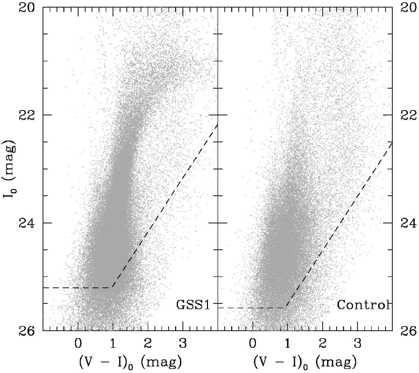
Figure 8.— Color-magnitude diagrams in the $I_{0}$ vs. $(V-I)_{0}$ plane for GSS1 and the Control Field (SE3). The dashed lines denote the full ranges of the 50% completeness levels for the mosaic images of the Suprime-Cam. Extended background galaxies have been removed via image classification.

To extract the detailed distribution of stellar populations in the GSS alone, the field stars other than the stream stars must be removed from the CMDs. For this purpose, we have made statistical subtraction of the field stars taken from the CMD of the control field, following the method by Durrell et al. (2004). In Figure 9, we show a colored contour for the log-scaled CMD of GSS1 field after this procedure, illustrating detailed characteristic features of the GSS stellar populations (cf. Bellazzini et al., 2003). It follows from this figure that in addition to the RGB feature, we identify a Red Clump (RC) at $I\sim 24.5$, structure in the CMD consisting of a number of helium core burning stars. More accurate estimates of the RC magnitude will be made below, by correcting for the incompleteness of magnitudes (Sec. 3.4). The detection of a clear RC thus indicates the presence of metal-rich and/or young populations in the GSS.

In Figure 9, there is also a second peak at $I\sim 23.5$, which is apparently brighter than the RC. This feature can be regarded as an Asymptotic Giant Branch (AGB) bump, not a RGB bump. This is for the reason that while most stars in the GSS appear to be old and/or metal-rich populations, a RGB bump with such old and/or metal-rich populations lies at a fainter magnitude than a RC magnitude in the CMD, following various theoretical models as calibrated by Alves & Sarajedini (1999). There is also a possibility that a clumpy feature being slightly brighter than a RC is just a portion of the red horizontal branch (RHB) clump as shown in Bellazzini et al. (2003). Their G76 field having such a feature is located at an edge of a luminous thin disk of M31, so only young, metal-rich populations like disk stars give rise to this kind of a feature slightly brighter than a RC magnitude.

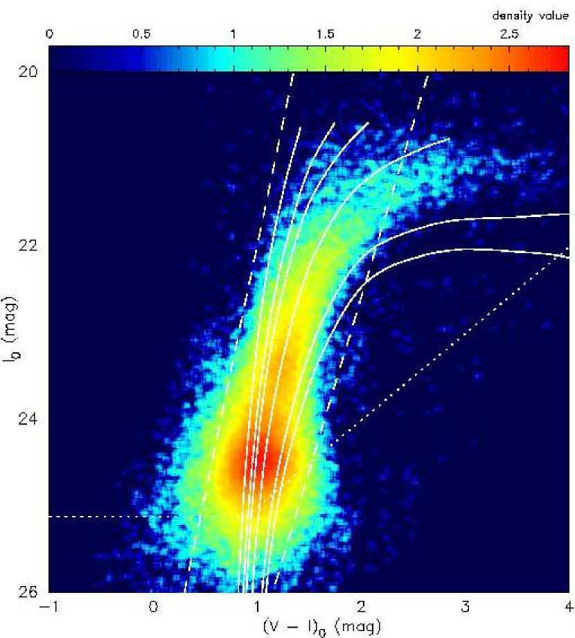
Figure 9.— A log-scaled CMD for GSS1. The peak number densities of the AGB bump and the RC amount to 224 and 657 stars per 0.07 $\times$ 0.07 mag box, respectively. Stellar density increases with redder color. The main features are distinguished by an edge of stellar density: the TRGB at $I_{0}\sim 20.5$ and by the reddest peaks of high stellar density: the AGB bump at $I_{0}\sim 23.5$ and the RC at $I_{0}\sim 24.5$. The solid lines are theoretical isochrones (VandenBerg et al., 2006) of age 12 Gyr spanning the metallicity range [Fe/H]$=-2.14$, $-1.41$, $-1.14$, $-0.71$, $-0.20$ and $0.00$. The dotted line denotes the full ranges of the 50% completeness level. Stars in the region between the two dashed lines are used to determine the edge of the TRGB and the peaks of the AGB bump and the RC in the following section.

At $I\sim 20.5$, we also recognize the tip of the RGB (TRGB). The presence of a few stars brighter than the TRGB magnitude level presumably suggests the presence of long-period variable stars in metal-rich and/or young population like bright AGB stars, as is the case in the halo of NGC 5128 (Rejkuba et al., 2003).

3.2. Distance to the Andromeda Giant Stream

As mentioned above, the TRGB is a useful indicator to estimate the distance to resolved galaxies (e.g., Lee et al., 1993; Madore & Freedman, 1995; Ferrarese et al., 2000; Salaris & Cassisi, 2005). If there are a sufficient number of old and metal-poor RGB stars in a targeted field, the TRGB is easily detected as a sharp cut-off of the luminosity function (LF) with the application of an edge detection algorithm, Sobel filter with a kernel $[-1,-2,0,+2,+1]$ (Madore & Freedman, 1995; Salaris & Cassisi, 2005). In this manner, we have identified the magnitudes of the TRGB from $I$-band LFs and determined the distance to the GSS. The TRGB is safely detectable, since it is bright enough not to be affected by incompleteness (i.e., more than 95% completeness for both $V$ and $I$-band magnitudes near the TRGB) and since it is fainter than a saturation level ($I\sim 19.5$) of the CCDs.

Detection of the TRGBs for the GSS1 field is shown in Figure 10 (see also Fig. 14). These smoothed LFs are constructed from the raw catalog by treating each star as a unit Gaussian with width $\sigma(I)$ and summing all the Gaussians (Durrell et al., 2001). Taking into consideration that the $I$ magnitude of the TRGB changes only by less than 0.1 mag for a metallicity range of $-2.2<$ [Fe/H] $<-0.7$ dex (Lee et al., 1993), which corresponds to the color range defined by the RGB of the metal-poor globular cluster NGC 6341 and metal-rich one 47 Tuc, we select the stars in this color range (between two dashed lines plotted in Figure 9) to estimate TRGB magnitudes. We then calibrate a residual LF, for which contaminations are removed by comparison with the LF of the control field. As deduced from Figure 10, the final selected LFs of the GSS’s stars show the leading edge of the LFs, indicating that the number density of RGB stars significantly exceeds the Poisson noise. In fact, the location of the TRGB on the LF is at the point that the contamination-subtracted LF with the vertical Poisson noise drawn in the middle panel of Fig. 10 is the most steeply rising up from the noise. Also, as shown later in Figure 14, the global shape of the LFs allows us readily to identify the TRGB.

Table 2 shows the distance to our two stream fields, on the assumption that the absolute $I$-band magnitude of the TRGB is $M_{I}^{\rm TRGB}=-4.1\pm 0.1$ for metal-poor TRGB stars. This $M_{I}^{\rm TRGB}$ adopted here corresponds to the $I$-band brightness of the TRGB at [Fe/H] $=-1.3$ derived from various empirical and semi-empirical calibrations (Ferrarese et al., 2000; Ferraro et al., 2000; Lee et al., 1993; Salaris & Cassisi, 1998) by Salaris & Cassisi (2005). The TRGB absolute magnitude suffers from statistical uncertainty of the order of $\sim$ 0.1 mag in each data. In estimating the extinction-corrected apparent magnitude of TRGB, $I_{\rm 0,TRGB}$, systematic errors also arise, related to zero point uncertainties, calibration through relative photometry, aperture corrections, photometric errors, smoothing of the LFs and extinction law; the resulting total error is evaluated by a root-mean-square of these errors.

Our estimated distance to the GSS in the GSS1 field is $883\pm 45$ kpc (see Tab. 2). It suggests that the GSS is located behind M31 (which is at $\sim 770$ kpc by Freedman & Madore (1990)) and extended along the line of sight, which is in good agreement with the distance to Field 5 in McConnachie et al. (2003) within errors ($840\pm 20$ kpc), the closest field to GSS1.

Table 2Distance to the GSS by analysis of the TRGB

Name	$I_{\rm 0,TRGB}$	Distance Modulus	Distance (kpc)
GSS1	$20.63\pm 0.05$	$24.73\pm 0.11$	$883\pm 45$

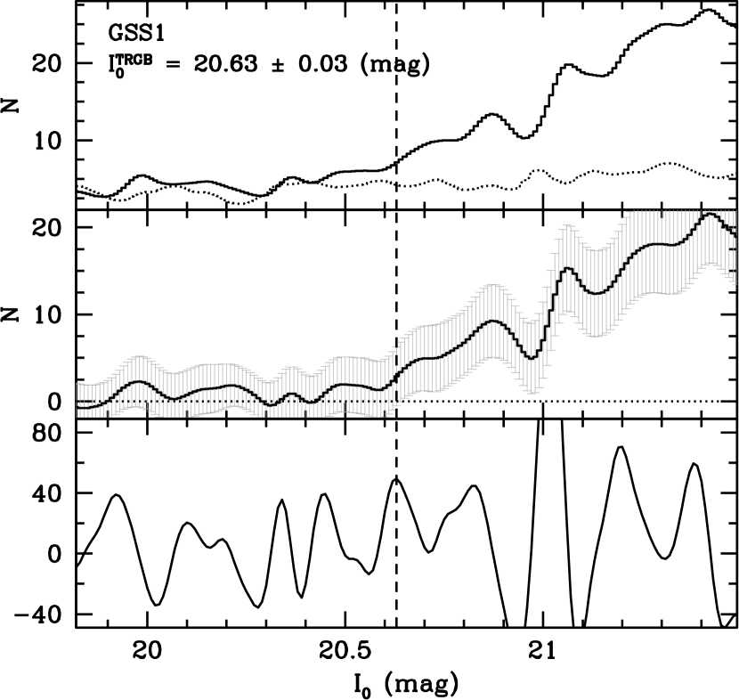
Figure 10.— TRGB detection in the GSS. The top panel presents the smoothed LFs as a function of the extinction-corrected $I$-band magnitude zoomed in around the TRGB magnitude. The solid line shows the original GSS1 LF before subtracting the background and the dotted line shows the background LF (which is the SE3 field). The middle panel shows the backgrond-subtracted GSS1 LF with Poisson error bars. The bottom panel indicates the Sobel filter response to the background-subtracted LF. The TRGB magnitude (the vertical dashed line) including the smoothing error is also shown.

3.3. Metallicity Distributions

We derive the metallicity distribution (MD) of the RGB stars in the GSS, based on the comparison with the RGB templates defined by Galactic globular clusters (Bellazzini et al., 2003). In this procedure, the assembly of a sufficient number of the RGB stars with small photometric errors is important for deriving an accurate MD, otherwise large photometric errors lead to the contamination of red or metal-rich stars; our Suprime-Cam data combined with the careful correction for contaminations shown in § 2.3.2 are advantageous in this respect. It is also remarked that recent studies by Brown et al. (2006a, b) suggest an intermediate age, i.e., younger than 10 Gyr, for about half the population of the GSS stars, in contrast to Galactic globular clusters. However, for low-mass RGB stars with age of 6-14 Gyr, the redward shift of an RGB sequence with increasing age is minor, compared with its sensitive redward shift with increasing metallicity (Girardi et al., 2002). This is a favorable behavior of the RGB, lending support to our procedure of deriving an MD in comparison with old globular clusters, but the photometric results should be followed up by spectroscopic observations.

As RGB templates we adopt the six ridge lines of Galactic globular clusters as in Bellazzini et al. (2003). The metallicities of these clusters are calibrated in the Carretta & Gratton (1997) abundance scale, hereafter denoted as $\rm[Fe/H]_{CG}$. We take four metal-poor clusters in the Galactic halo from Saviane et al. (2000): NGC 6341 ($\rm[Fe/H]_{CG}=-2.16$), NGC 6205 ($\rm[Fe/H]_{CG}=-1.39$), NGC 5904 ($\rm[Fe/H]_{CG}=-1.11$) and 47 Tuc ($\rm[Fe/H]_{CG}=-0.70$). In addition, we take two metal-rich clusters in the Galactic bulge, NGC 6553 ($\rm[Fe/H]_{CG}=-0.16$) from Sagar et al. (1999) and NGC 6528 ($\rm[Fe/H]_{CG}=0.07$, Carretta et al., 2001) from Ortolani et al. (1995) (see Table 3). For secure determinations of MDs using these templates, we select the targeted RGB stars having $-3.8<M_{I}<-2.0$ and $0.9<(V-I)_{0}<4.0$ as shown in Figure 11. These selection criteria also allow us to remove a number of contaminations, such as AGB stars, AGB bump stars, young stars, and foreground and/or background objects. We perform the interpolation procedure to obtain the metallicities of the stars both in the stream and control fields, and subtract the derived distribution of metallicities in the control field from that in the stream field in order to remove the effects of the M31 field halo stars.

Table 3Galactic globular cluster data used in the present study

	[Fe/H]CG	$E(B-V)$	$(m-M)_{0}$
NGC 6341  M92	$-2.16$	$0.02$	$14.74$
NGC 6205  M13	$-1.39$	$0.02$	$14.38$
NGC 5904  M5	$-1.11$	$0.03$	$14.31$
NGC 104  47Tuc	$-0.70$	$0.04$	$13.29$
NGC 6553	$-0.16$	$0.84$	$13.44$
NGC 6528	$~{}~{}~{}0.07$	$0.62$	$14.35$

Note. — The metallicities of these clusters are calibrated in the Carretta & Gratton (1997) abundance scale.

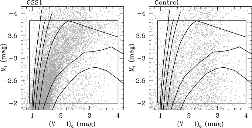
Figure 11.— CMDs of the upper RGB part for two fields. The ridge lines of template Galactic globular clusters are superimposed to each plot as solid lines, which are from left to right, NGC 6341 ([Fe/H]$=-2.16$), NGC 6205 ([Fe/H]$=-1.39$), NGC 5904 ([Fe/H]$=-1.11$) and NGC 104 ([Fe/H]$=-0.70$), NGC 6553 ([Fe/H]$=-0.16$) and NGC 6528 ([Fe/H]$=-0.07$). The inner square frame encloses the stars whose metallicities are determined using the interpolating scheme (Bellazzini et al., 2003).

Figure 12 shows the MDs in the GSS1 field of the GSS. The vertical error bars denote a nominal uncertainty in each metallicity bin, derived from the Poisson errors equal to $\pm\sqrt{N({\rm stream}+{\rm control})}$. It is worth noting that these errors are significantly small because of a large number of the RGB stars (7051 stars in the GSS1 field) available from our Suprime-Cam data. It follows that the MDs have a broad distribution ranging from [Fe/H] $\sim-3$ to the near solar metallicity and there is a clear high-metallicity peak at [Fe/H]${}_{\rm peak}\sim-0.3$. In the GSS1 field, the average metallicity is [Fe/H]${}_{\rm mean}=-0.55\pm 0.45$ and the median metallicity is [Fe/H]${}_{\rm med}=-0.45$ with a quartile deviation of 0.23 dex. The average metallicities derived here are in good agreement with those of kinematically selected RGB stars in the GSS (Guhathakurta et al., 2006; Kalirai et al., 2006b).

Figure 12.— Metallicity distribution for the GSS1 field. The number of stars used to derive it are shown in the upper left corner of the panel. The average metallicity with the standard deviation and the median metallicity with the quartile deviation of the GSS1 field are shown in the panel.

While the MD is dominated by metal-rich stars, the presence of metal-poor stars reaching [Fe/H]$\leq-2$ is suggested from a long metal-poor tail in the MD, based on the existence of an extended blue horizontal branch in the CMDs derived by HST/ACS (Ferguson et al., 2005; Brown et al., 2006a, b). Our found metal-poor tail feature is consistent with Bellazzini et al. (2003). However, as the also discussed, we cannot strongly claim really and scattered RGB stars with [Fe/H]$\geq-2$.

3.3.1 Effects of Adopted Assumptions on Metallicities

The detailed form of the MDs is affected by several assumptions in the analysis, such as adopted distance modulus $(m-M)_{0}$ and reddening correction $E(B-V)$. To see these effects in the MDs, we examine the GSS1 field as an example and the results are shown in Figure 13. While Fig. 12 shows the case based on our standard assumptions, the left four panels in Figure 13 show the MDs associated with the change of our assumptions. For reference, we also plot the MD derived based on the standard assumptions as the dotted histogram. Panels (a) and (b) are devoted to the effect of changing $\pm 0.11$ mag in distance modulus, resulting in the change of mean/median metallicity at only $\pm 0.07$ dex level. Somewhat large change of the MDs is seen in panels (c) and (d), where we test $\pm 0.05$ mag variation in $E(B-V)$. This is inevitable because our method for deriving MDs is based on the comparison between the color distributions of RGB stars and that of adopted templates, thereby a change of $E(B-V)$ affects this comparison in a sensitive manner, especially in a metal-poor range below [Fe/H] $=-1$, where the dependence on color is large. The resultant change in metallicities is however no more than $\pm 0.18$ dex in response to a $\pm 0.05$ mag change in $E(B-V)$.

Next, we examine the effect of adopting different RGB templates, i.e., other than Galactic globular clusters, to estimate the metallicity of each star. To do so, we re-construct the MDs using the Victoria-Regina theoretical isochrones from VandenBerg et al. (2006) (whose isochrones are partly displayed in Fig. 9), in place of the globular cluster templates of the Milky Way. In accordance with the interpolation and extrapolation scheme of Kalirai et al. (2006b), we calculate the metallicity for each star in the same segment of the CMD (see also their Fig. 6). The resultant MDs with different $\alpha$-enhancement, distance modulus and age are shown in the right four panels of Figure 13. Panels (a) and (b) are devoted to the effect of changing 4 Gyr in age, resulting in the change of mean/median metallicity at approximately $0.1$ dex level. Somewhat large change of the MDs is seen in panels (a) and (c) with the two different [$\alpha$/Fe]. The MD with $\alpha$ no-enhancement is very similar to the one derived from the Galactic globular cluster templates, while the $\alpha$-enhancement MD has a more metal-poor peak. Finally, in panels (a) and (d), we test the effect of varying distance modulus. The difference of mean metallicity between the two is 0.06 dex. The four MDs derived from the model have gradual increase to the peak at [Fe/H] $\sim-0.3$ without sharp edge at [Fe/H]$\sim-1.1$ and $-0.7$ as in MDs constructed based on the Galactic globular cluster templates, although all the MDs derived from different metallicity indicators have the same global shape such as the high metallicity peak at [Fe/H] $\sim-0.3$, the existence of stars with near solar metal and the long metal-poor tail. Furthermore, the GSS’s mean metallicity shown in panel (a) of the right of Figure 13, where the basic assumptions behind this is almost the same as those of Brown et al. (2006b), is in good agreement with the mean metallicity of $\langle$[Fe/H]$\rangle=-0.7$ derived from their best-fit model (based on the distance modulus of 780 kpc and the Victoria-Regina isochrones). It is noteworthy that our mean metallicity estimated from only RGB stars is consistent with their result by main-sequence fitting to much deeper CMD.

Based on these experiments, we conclude that the basic features of the MDs derived here are robust, including the existence of stars with near solar metallicities, high metallicity peak at [Fe/H]$\sim-0.3$, and long metal-poor tail. The mean and median metallicities remain basically unchanged within a typical error of at most 0.1 to 0.2 dex in the current method.

Figure 13.— Effects of varying assumptions on the form of the MDs. The dotted histogram: our standard case with $(m-M)_{0}=24.43$ and $E(B-V)$ from the Schlegel et al. (1998) map, which is derived based on the Galactic globular cluster templates. Left: Panel (a): $(m-M)_{0}$ increased by 0.15 mag, (b): $(m-M)_{0}$ decreased by 0.15 mag, (c): $E(B-V)$ increased by 0.05 mag, and (d): $E(B-V)$ decreased by 0.05 mag. Right: Re-constructed MDs based on the Victoria-Regina theoretical isochrones from VandenBerg et al. (2006) with the change of [$\alpha$/Fe], $(m-M)_{0}$ and age.

3.4. Stellar Populations Inferred from the AGB Bump and Red Clump

In addition to the broad RGB feature of the GSS, being attributable to a composite population of metal-rich and metal-poor stars, the CMD shows two noticeable populations (see Fig. 9), the AGB bump and RC, which are related to more advanced stellar evolutionary phases. To highlight these features, we show, in Figure 14, the $I$-band LFs of the GSS1 field, which are corrected for extinction. The dashed and solid lines denote LFs before and after correction for incompleteness, respectively. The vertical dotted line indicates a 50 % completeness magnitude of $I_{0}=25.22$ for the GSS1 field. The main features are marked by vertical solid lines: the TRGB, AGB bump, and RC. More details on the latter two features are discussed below.

Figure 14.— $I$-band luminosity function corrected for extinction and incompleteness at magnitude brighter than horizontal branch of GSS1 field, is plotted with solid line, while the dashed curve shows the curve with extinction-correction only. The vertical dotted lines indicate 50% completeness magnitude of $I_{0}=25.21$ for GSS1 field. The main features are indicated by vertical solid lines: the TRGB at $I_{0}\sim 20.63$, the AGB bump at $I_{0}\sim 23.37$, and the RC at $I_{0}\sim 24.52$.

3.4.1 AGB Bump

The AGB bump is a stellar evolutionary phase of low-mass stars, and is caused by the clustering of stars in a CMD, where AGB stars at the beginning of helium shell-burning evolution slowly re-ascend along the Hayashi line in a thermal nonequilibrium state. However, due to the very short lifetime of the AGB phase, the AGB bump feature can be detected only when dealing with a large sample of stars (Rejkuba et al., 2005). In fact, Gallart (1998) first detected an AGB bump from the data of Holland et al. (1996) in the dense inner part of M31’s halo (at 7.6 kpc from the center approximately along the SE minor axis). As already reported in § 3.1, we have also found an AGB bump feature in the stream field at $I_{0}\sim 23.5$ and $(V-I)_{0}\sim 1.2$ (Fig. 9).

To more quantitatively identify the mean magnitude of the AGB bump, we perform a Gaussian-weighted fit to the $I$-band LF of GSS stars after correction for extinction and incompleteness. The upper left and right panels of Figure 15 shows the zooming CMD and the LF with Poisson errors for the GSS1 field near the AGB bump magnitude, respectively. In this procedure, the surrounding stars in the shaded zones (left-hand panel) are avoided to reduce unwanted contaminations, since the AGB bump feature is rather weak. At the magnitude level of the AGB bump, our photometric completeness is more than 80 % for $I$-band imaging. Although, in the usual CMD of the left panel, it is somewhat difficult for us to detect the AGB bump feature by eye, we can easily confirm the existence of the stellar population specified by the AGB bump through the LF of the right panel. A red solid curve drawn in the LF is the best-fit model with the sum of a Gaussian function and a straight line in the range of $23.1\lesssim I_{0}\lesssim 23.8$. The best-fit function has been derived by minimizing reduced chi-squares in the fitting procedure. The mean magnitude of the AGB bump is then derived from an average value from these fittings: for the GSS1 field this is $I_{0}=23.37\pm 0.16$, corresponding to $M_{I}^{\rm AGBb}=-1.37$ with a standard deviation of 0.13 mag. The estimation of this error is based on those in the photometry, smoothing and fitting procedures as well as the distance error using the TRGB as shown in $\S$ 3.2. We note that the fitting error in the GSS1 field is negligibly small (less than $0.01$ mag).

3.4.2 Red Clump

The RC is a clustering feature of RHB stars being metal-rich and/or intermediate-age. HST/ACS observations (Brown et al., 2006a, b) of the stream field, which is located closer to the galactic center than ours, suggest the dominance of RHB stars in the HB, i.e., the presence of RC. We have also found this feature in our stream fields, as already reported in § 3.1, at $I\sim 24.5$ and $(V-I)\sim 1.0$ (Fig. 9).

As in the case of the AGB bump, we set tighter limits on the mean magnitude of the RC based on a Gaussian-weighted fit to the suitably corrected $I$-band LF. The bottom left and right panels of Figure 15 shows the zooming CMD and the LF near the RC magnitude, as in the upper panel of Figure 15 for the AGB bump. We note that particular attention must be paid to the magnitude completeness since the RC is just beyond the detection limit: the completeness at RC is about 60 % for $I$-band image. We thus reconstruct the completeness-corrected LF, using the completeness curves for the stars in the unshaded zone of the CMD (the bottom left-hand panel of Figure 15). A red solid curve drawn in the LF is the best-fit model with the sum of a Gaussian and a straight line in the range of $23.8\lesssim I_{0}\lesssim 24.9$. Using the curve we determine the mean magnitude of the RC: for the GSS1 field this is $I_{0}=24.52\pm 0.22$, corresponding to $M_{I}^{\rm RC}=-0.21$ with the standard deviation of 0.17 mag. This error is derived in the same manner as for the AGB bump; in this case the photometric uncertainty is larger.

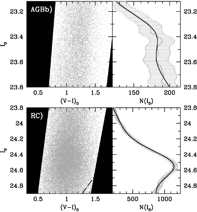
Figure 15.— Zoom up display of the CMD of the GSS1 field around the AGB bump and the RC features referring to Rejkuba et al. (2005). We do not use the stars in shaded areas to evaluate the luminosity functions (see text). Shown on the right panels are the $I_{0}$-band completeness-corrected LFs around the AGB bump and the RC, best-fitted with a simple model comprising of a Gaussian plus a straight line. The peaks of the AGB bump and the RC for the GSS1 field are at $I_{0}=23.37\pm 0.16$ with $\sigma=0.13$ and $I_{0}=24.52\pm 0.22$ with 0.17, respectively.

3.4.3 Age Estimation

We estimate the mean age of the GSS’s stars using the relation between age and metallicity for the AGB bump and RC features. For this purpose, we adopt the calibration of this relation by Rejkuba et al. (2005) using the theoretical stellar evolutionary tracks of Pietrinferni et al. (2004). Applying to their observations of NGC 5128’s halo, they showed that the mean age of the halo stars in NGC 5128 is estimated as $\sim 8^{+3}_{-3.5}$ Gyr.

Figure 16 shows the absolute $I$-band magnitudes of the AGB bump and RC features predicted by the theoretical models, plotted as a function of age for five different metallicities. The horizontal dotted lines show the measured absolute magnitudes of the AGB bump and RC, respectively. If we assume that the alpha elements of the GSS’s stars are enhanced such that [$\alpha$/Fe] $=+0.3$ as seen in the local halo stars of the Milky Way, where the conversion, [M/H]$\sim$[Fe/H]$+0.3$, holds for most metallicity ranges, the average metallicity of the stream fields is estimated as [M/H] $=-0.25$, which suggests (as seen from asterisks in the Figure) the average age of the GSS stars of $\sim 8$ Gyr.

Figure 16.— Absolute $I$ magnitudes of the AGB bump and RC features predicted by the theoretical models, plotted as a function of age for five metallicities (kindly provided by Dr. Marina Rejkuba). These metallicities cover most of the metallicity range of the observed MD in the halo of the GSS. For comparison, the measured AGB bump and RC magnitudes are indicated with horizontal dotted lines.

To be more quantitative, we compute the average magnitude of the AGB bump and RC as a function of age, as expected for the observed MDs using equation (9) of Rejkuba et al. (2005). Figure 17 shows the corresponding average $I$ magnitudes of AGB bump and RC features plotted as a linear function of age, where the error bars are evaluated by employing $\pm 0.1$ dex shift in the observed MDs. The dotted horizontal lines indicate the measured mean magnitudes of the AGB bump and RC. These magnitude measurements have a negligible statistical error due to a huge number of available stars, but they contain a systematic error associated with reddening and distance uncertainties, which amounts to about $\pm 0.22$ mag. It is worth noting that for metal-poor and old populations with [M/H] $<-1$ and age of $>9$ Gyr, the AGB bump feature is invisible in the theoretical luminosity functions, and only a very weak feature is present for more metal-rich stars (Rejkuba et al., 2005), so the model predictions for the AGB bump with older ages are not shown.

Figure 17.— Absolute $I$ magnitudes of the AGB bump and RC features vs. age predicted by the theoretical models, as obtained by convolving the metallicity dependency with measured metallicity distributions of the RGB stars (see Rejkuba et al., 2005). Filled circles present the relations computed with [$\alpha$/Fe] $=+0.3$, while open circles indicate those computed with no $\alpha$-enhancement. The measured AGB bump and RC magnitudes are shown as dotted horizontal lines. The error bars on the model points are calculated from assumed $\pm 0.1$ dex uncertainty in the measured metallicity distributions.

The mean magnitude of the RC in GSS1 field indicates that the average age of stars is 7.1 Gyr, whereas the AGB bump magnitude in the field suggests younger age. However, as seen in Figure 17, the dependence of the AGB bump magnitude on age is much weaker than that of the RC, so that small systematic errors in the measured AGB bump magnitude can lead to a large difference in the estimated age. The abundance of $\alpha$ elements somewhat affects the AGB bump-based age estimation, in such a manner that lower [$\alpha$/Fe] ratios yield older ages (see open circles for [$\alpha$/Fe]$=0$ in Fig. 17), whereas the RC-based age estimation is rather insensitive to this effect. Much larger systematics may be caused by the followings: (1) The AGBb feature appears only when [M/H]$>-1$ and age of $<9$ Gyr, so the mean age of the stars is dominated by relatively metal-rich and thus bright populations. (2) If the GSS contains relatively young populations associated with secondary star formation activities, the mean luminosity of the AGBb reflects the relative fraction of each population, especially being biased in favor of younger, brighter populations. This effect would be more significant for AGBb than RC, because the number of the stars in the AGBb feature is much small, so the Poisson error in the number of the populations, especially for the small number of bright stars among the AGBb stars is relatively large, thereby having a larger probability of yielding a brighter AGB magnitude and younger ages.

Thus, while taking into account that AGB bump magnitudes yields younger ages, we adopt the RC-based age estimation, giving upper limits on the age of GSS stars. Based on the available $I$-band magnitude of the RC (because its $V$-band magnitude is unavailable in the current study), we arrive at $7.1_{-4.7}^{+3.6}$ Gyr for the mean age of GSS stars, where the error includes 0.22 mag systematic uncertainties in the RC magnitude arisen from reddening, distance modulus and so on, while the uncertainties in stellar evolutionary models are not taken into account. Rejkuba et al. (2005) compared Teramo models (Pietrinferni et al., 2004) with Padova models (Girardi et al., 2000) in their similar study for the stellar population of NGC 5128 and found an additional 1 Gyr uncertainty due to the age difference between the two model predictions.

We note that the mean age of GSS stars derived from the RC magnitude is slightly younger compared to that derived by Brown et al. (2006b). They estimated the GSS’s mean age to be 8.7 Gyr and the mean metallicity to be $\langle$[Fe/H]$\rangle=-0.7$ based on the main-sequence fitting with the distance modulus of 780 kpc and the Victoria-Regina isochrones, whereas our re-computed mean age based on the MD constructed by the Victoria-Regina theoretical isochrones (where the MD is shown in the panel (a) of the right of Fig. 13) is 8.1 Gyr. This result is consistent with the GSS’s mean age found by Brown et al. (2006b). In addition, the mean age and metallicity estimations based on different assumptions as discussed in § 3.3.1 are listed in Table 4. In particular, all mean ages derived from the AGB bump magnitude are much younger than those derived from the RC magnitudes. The theoretical models provide robust mean ages without assumptions such as $\alpha$-enhancement and age to estimate the metallicity, while the ages are somewhat sensitive to the assumption of distance as well as in the case of using the Galactic globular cluster templates. Therefore, we note that our technique applied to calculation of mean age based on the RC magnitudes produces several Gyr uncertainty in accordance with assumptions such as distance, extinction, $\alpha$-enhancement and stellar evolutionary models.

The use of the AGB bump magnitude suggests systematically younger ages, although this age estimation is rather sensitive to the accurate determination of the AGB bump magnitude. We note that the presence of the AGB bump feature implies the dominance of young and metal-rich populations in the GSS; Rejkuba et al. (2005) reported that in the models with ages $\hskip 3.00003pt\raisebox{1.72218pt}{$>$}\raisebox{-3.01385pt}{$\sim$}\hskip 3.00003pt10$ Gyr there exist very few AGB bump stars compared to the RC or horizontal-branch stars and that in metal-poor ([M/H]$<-1$ dex) and old (age $>9$ Gyr) models the AGB bump is not present at all. Thus, the presence of the AGB bump itself yields the younger age estimate. It is also noted that the current implication for young and metal-rich populations in the GSS may be associated with the result of Brown et al. (2006b) (as depicted in their Figure 17b), suggesting that star formation activities in the GSS had continued until some Gyrs ago; it is inferred that the progenitor of the GSS may have had three main star formation activities: (1) 30% of the stars were provided in the first star formation (e.g., by the collapse of the initial gas) before 8 Gyrs ago, (2) 40% of the stars were provided in the second star formation (e.g., supernova feedback or galactic interactions) about 8 Gyrs ago, and (3) remaining 30% of the stars were provided in the third star formation (e.g., the tidal interaction in the first pericentric encounter with M31) after the second star formation.

3.5. Mass of the Progenitor Galaxy

The total mass of the stellar system expected for the progenitor galaxy of the GSS can be estimated from the mean metallicity of stars in the GSS ([Fe/H]${}_{\rm mean}=-0.7$), combined with the metallicity-luminosity relation for Local Group dwarfs (Côté et al., 2000). The relation shows, on average, more metal-rich populations in more luminous galaxies, and we obtain $M_{\rm stars}\sim 10^{7}$ M_⊙ for the progenitor galaxy if the mass-to-light ratio is $M/L\sim 2$. In contrast, assuming the stellar mass-metallicity relation observed for the Local Group dwarf galaxies of Dekel & Woo (2003), we find $M\sim 4\times 10^{9}M_{\sun}$ as the progenitor mass, which is consistent with the work of Mori & Rich (2008) who restricted the progenitor mass to be $M\leq 5\times 10^{9}M_{\sun}$, taking into account the effect of disk heating by dynamical friction. Such a dwarf galaxy may have been accreted to the M31 halo at recent epochs, possibly within some billion years, leaving yet a conspicuous giant stream like the Sgr stream in the Milky Way.

Table 4Mean age and metallicity based on various assumptions

Various Assumption	$\langle$[Fe/H]$\rangle$	$\langle$age$\rangle_{\rm RC}$	$\langle$age$\rangle_{\rm AGBb}$
Based on the Galactic globular cluster templates
Standard	$-0.55$	$7.1$	$0.7$
Standard with no $\alpha$-enhancement	$-0.55$	$8.2$	$2.3$
$(m-M)_{0}+0.11$ (24.84)	$-0.62$	$4.8$	$1.0$
$(m-M)_{0}-0.11$ (24.62)	$-0.49$	$9.4$	$2.8$
$E(B-V)+0.05$ (0.10)	$-0.73$	$5.6$	$0.4$
$E(B-V)-0.05$ (0.00)	$-0.42$	$8.9$	$1.4$
Based on the Victoria-Regina theoretical isochrones
$[\alpha$/Fe$]=+0.3$, dm$=24.73$, 8 Gyr	$-0.68$	$8.0$	$1.9$
$[\alpha$/Fe$]=+0.3$, dm$=24.73$, 12 Gyr	$-0.79$	$8.1$	$2.3$
$[\alpha$/Fe$]=+0.0$, dm$=24.73$, 8 Gyr	$-0.55$	$8.2$	$2.5$
$[\alpha$/Fe$]=+0.3$, dm$=24.62$, 8 Gyr	$-0.62$	$9.4$	$4.9$

4. Panoramic Views of the Andromeda Stellar Halo

In this section, we report on the results for the entire halo regions of M31 observed by the current survey, i.e., including those along its minor axis both in the north and south parts of the galaxy and a south-west major-axis region.

4.1. The Color-Magnitude Diagram

Figure 18 shows a co-added CMD from all of the observed fields (including the GSS field as shown in the previous section), after removing extended sources such as background galaxies and cosmic rays based on DAOPHOT parameters (see § 2.3.2). The thin solid lines in the CMD show theoretical RGB tracks from VandenBerg et al. (2006) for an age of 12 Gyr, [$\alpha$/Fe]$=+0.3$, and metallicities (left to right) of [Fe/H]$=-2.31$, $-1.71$, $-1.14$, $-0.71$, $-0.30$ and $0.00$. The dotted line denotes about 90 % completeness limit as determined by artificial star experiments, where the limit is estimated by making use of the NW8 field with worse seeing and shorter exposures. Although redundant stars and galaxies are not completely removed from the CMD, we can clearly identify a broadly distributed RGB feature attributable to overdense regions with a number of metal-rich stars such as the GSS. At fainter than $I_{0}\sim 23$ (mag), the RGB feature appears to be much broader because of the presence of background galaxies which passed through our selection of separate stellar objects. Although it is contaminated by these objects, a population extending toward fainter and bluer region than the most metal-poor theoretical RGB isochrone at $I_{0}\gtrsim 24$ (mag) corresponds to the horizontal branch stars in M31’s halo.

In the right panel of Fig. 18 which is the same CMD as the left one but with the higher maximum level of representation in the stellar densities, there exists a sequence of Galactic disk dwarfs at $(V-I)_{0}\gtrsim 2$ having a broad RGB; the vertical sequence is the result of low-mass stars accumulating in a narrow color range, yet being seen over a large range in distance along the line of sight. In addition, halo stars in the Milky Way can be seen as vertically-distributed stars on the blue side of this diagram, $(V-I)_{0}\lesssim 0.8$ and $I_{0}<23$. Usually this appears as a smooth vertical structure in a CMD, which corresponds to the stars at or close to the main-sequence turnoff at increasing distance through the Galactic halo (Martin et al., 2007; Ibata et al., 2007).

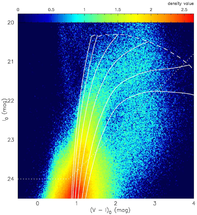
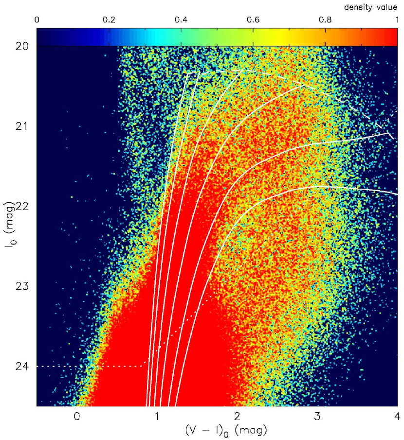
Figure 18.— A composite CMD in the $I_{0}$ vs. $(V-I)_{0}$ plane for stellar sources detected in all the observed fields (including the GSS field). The dotted lines denote the full range of the 90% completeness levels for the mosaic images of the Suprime-Cam in the NW8 field. The superposed solid lines in the CMD show theoretical RGB tracks from VandenBerg et al. (2006) for an age of 12 Gyr, [$\alpha$/Fe]$=+0.3$, and metallicities (left to right) of [Fe/H]$=-2.31$, $-1.71$, $-1.14$, $-0.71$, $-0.30$ and $0.00$. Extended background galaxies have been removed via image classification. The right panel is the same CMD as the left panel, but with the higher maximum level of representation in the stellar densities.

4.1.1 Calibration of the Control Field

Our three control fields, to be utilized for removing contaminations such as Galactic dwarf stars which cannot be separated morphologically, are located at the same galactic longitude $l=103\arcdeg$ but at different galactic latitudes with $b=-16\fdg 5$, $-20\fdg 7$, and $-25\fdg 1$, i.e., far from the M31 direction ($l=121.2\arcdeg,b=-21.6\arcdeg$). The CMDs of the three control fields are shown in Figure 19; from left to right, galactic latitude is higher. For reference, the solid/dotted white lines as shown in Fig.18 are also plotted in these CMDs. A prominent feature is that the number of Galactic disk dwarf stars is gradually decreasing with increasing galactic latitudes. In contrast, there is little change in the distribution of remaining faint background galaxies between these three CMDs. Finally, it is found that the number variation of the Galactic halo stars in these CMDs is also small.

Figure 19.— CMDs of the three control fields in the $I_{0}$ vs. $(V-I)_{0}$ plane. For reference, the white solid/dotted lines as shown in Fig. 18 are also overlaid. left: $(l,b)=(103\fdg 0,-16\fdg 5)$, middle: $(l,b)=(103\fdg 4,-20\fdg 7)$, right: $(l,b)=(103\fdg 4,-25\fdg 1)$.

These properties of the control fields indicate that the contaminants in our target fields of M31’s halo are dominated by the faint background galaxies and the Galactic disk dwarf stars, while the effect of the Galactic halo stars can easily be corrected because such stars distribute outside the M31 RGB sequence in the CMD. Regarding the unresolved background galaxies, one can assume that such galaxies are uniformly distributed in a Suprime-Cam field-of-view, whereby these background contaminants per field are simply regarded as having a uniform density, regardless of the galactic latitude. Thus, the remaining task is to understand the effects of the foreground Galactic disk dwarf stars on our target fields.

In order to correct the effect of these dwarf stars in each target field of M31’s halo, we estimate the fraction of such stars in each target field based on the knowledge of the number of the contamination stars in the CMDs of the control fields, by combining the observed CMDs and those predicted by the models of Robin et al. (2003). Firstly, we use two CMDs of the short exposed NW1 field and one of the three control fields with almost the same galactic latitude of $b\sim-21\arcdeg$. We have obtained 0.78 as the scale factor to adjust the number difference arising from the galactic longitudinal difference between the M31 with $l\approx 121\arcdeg$ and our control fields with $l\approx 103\arcdeg$, based on the comparison of the star counts of clean Galactic dwarfs in a box defined as $17.0<I_{0}<18.0$ and $1.5<(V-I)_{0}<2.2$. Note that these selection criteria enable us to avoid the effects of bright AGB and RGB stars of M31. This scale factor derived from our observation is consistent with the model prediction from Robin et al. (2003) including Poisson noise. In addition, the scale factor calculated from the star count of the disk stars in a box defined as $20.5<I_{0}<22.5$ and $1.2<(V-I)_{0}<3.0$ of the corresponding model CMDs without the M31 population is also in good agreement with the scale factor from the comparison of the bright disk stars. Secondly, we investigate the variation of the number density of the disk dwarf stars along galactic latitude. Figure 20 shows the relative number variation normalized by the number at the control field with $b=-20\fdg 7$ as a function of the galactic latitude, where the disk stars reside in a box defined as $20.5<I_{0}<22.5$ and $1.2<(V-I)_{0}<3.0$. The three big solid circles denote our observed results, while the small solid circles show the model prediction by Robin et al. (2003) with the same galactic coordinates as our M31 target fields and the solid triangles are the scaled plots by the above-mentioned scale factor of 0.78. It is evident that the spatial variations of both the observational result and the model prediction are reasonably consistent with each other. Based on the results of these experiments, we thus adopt the theoretical galactic model of Robin et al. (2003) to estimate the spatial variation of the number of the disk dwarf stars. This spatial variation of the number density is well represented by an exponential profile at the lower galactic latitude than that of the NW1 field and is represented by a linear profile at the higher galactic latitude, as judged by a (dotted) fitting line in the figure. For this correction of the contaminations, we adopt the blank field with the lowest galactic latitude of $b=-16\fdg 5$ as the control field for the north part of the M31 halo, whereas the blank field with the galactic latitude of $b=-20\fdg 7$ is adopted as the control field for the south part of the M31 halo.

Figure 20.— The variation of the number density of the Galactic disk stars as normalized by that in the control field with $b=-20\fdg 7$ as a function of the galactic latitude. The disk stars are taken from a box defined as $20.5<I_{0}<22.5$ and $1.2<(V-I)_{0}<3.0$ in the CMD. The three big solid circles denote our observational results, while the small solid circles show the model prediction by Robin et al. (2003) with the same galactic coordinates as our M31 target fields and the solid triangles are the scaled plots. The solid triangles are fitted by exponential (at the lower latitude than that of the NW1 field) and linear profiles (at the higher latitude).

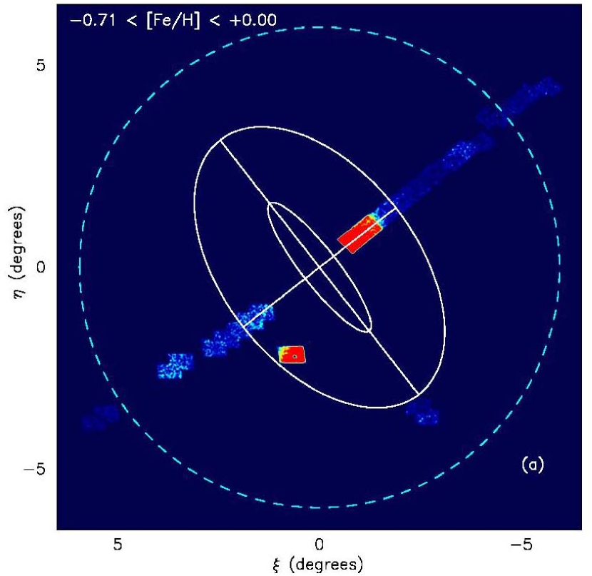
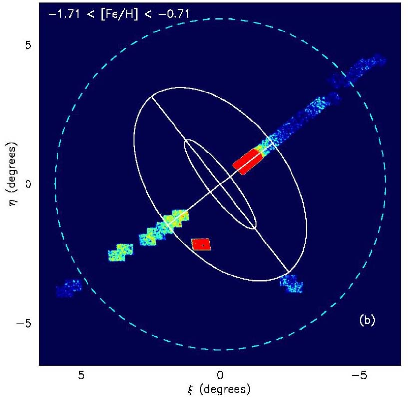
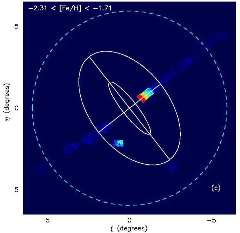
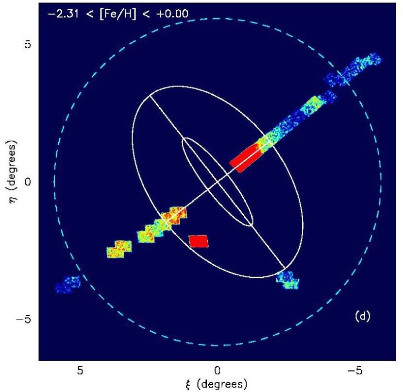
Figure 21.— Matched filter maps to a limiting magnitude of $I_{0}=24.0$ and $V_{0}=24.8$. Log-scaled images are shown on the left, while linear-scale versions are presented on the right. The resolution of this map is $0.018\arcdeg\times 0.018\arcdeg$ pixels, smoothed with a Gaussian kernel over 3 pixels.

4.2. Stellar Population Maps

In this subsection, we investigate how the RGB populations of the M31 halo, as identified in Fig. 18, are distributed spatially out to about 100 kpc from the M31 center. To do so, we extract these stellar populations of M31 alone from our imaging data. However, it is noted that the outer halo of M31 is known to have a very diffuse stellar density as deduced from previous studies (e.g., Gilbert et al., 2006; Irwin et al., 2005), so a clean signal of these M31 populations is buried under heavy contamination from foreground disk dwarf stars and the background galaxies. In particular, the amount of the disk dwarfs in the northern part of the M31 halo are about twice as much as in the southern region, as suggested in Fig. 20. In order to reveal the signal from these heavily contaminated data, we adopt the so-called matched filter method as has been utilized in Ibata et al. (2007). This method is an optimal search strategy if one has a precise idea of the properties of both the signal and the contamination.

We first divide the $I_{0}$ vs. $(V-I)_{0}$ plane into uniformly-spaced rectangular grids. Then, based on the simple weighting of each CMD in a box defined by these grids, in terms of the ratio of signal to contamination as expected for the concerned CMD, we can optimally boost the signal and suppress the contamination. Since we have the objective CMDs (i.e., containing both the signal and contamination) as well as the CMDs containing only the contamination, it is possible to obtain the so-called weight matrix, which is given by subtracting the CMD for the contamination from the objective CMD (using the correction method for the contamination as discussed in the previous subsection), and finally we sum up these corrected CMDs in each field of M31’s halo. The weight matrix obtained by this procedure is shown in Figure 22. This is reasonably similar to the one derived by Ibata et al. (2007). Here, to construct the weight matrix, we have selected the stars filed with 90% completeness limit, the fainter stars than an upper dashed line of Fig. 18 and the stars in the possible metallicity range of $-2.31<{\rm[Fe/H]}<+0.00$, as an example. Note that, as expected, the greatest weight arises at faint magnitudes in the color range of $0.9<(V-I)_{0}<1.5$, so of course, stars with this photometric property will contribute most strongly to the following matched filter maps.

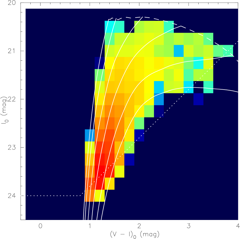
Figure 22.— Matched filter weight map on a log scale, trimmed to the color-magnitude region encompassing stars of metallicity $-2.31<{\rm[Fe/H]}<+0.00$. The resolution of this map is 0.2 (mag) $\times$ 0.25 (mag).

Based on this method, we have analyzed all of the CMDs and obtained the matched filter maps. In Figure 21, we present the final matched filter maps over the entire survey region for four different ranges in metallicity. The maps are smoothed with a Gaussian kernel over 0.054$\arcdeg$. The limiting magnitudes are chosen to be $I_{0}=24.0$ and $V_{0}=24.8$; these magnitudes keep the detection efficiency over 90% completeness in the entire region. The images with the resolution of $0.018\arcdeg\times 0.018\arcdeg$ are displayed in a logarithmic scale for the left panels, whereas the right panels are shown in a linear scale. The inner ellipse overlaid in these maps represents a disk of inclination $77\arcdeg$ and radius $2\arcdeg$ (27 kpc), the approximate end of the regular HI disk. The outer ellipse shows a $4\arcdeg$ (55 kpc) radius ellipse which is flattened to have the axis ratio of $c/a=0.6$ [i.e., standard guide ellipse firstly drawn by Ferguson et al. (2002)]. In addition, the cyan concentric dashed circles show projected radii of 80 kpc. We note that the logarithmic-scaled maps are useful for elucidating the global spatial variation of the M31 populations in the inner halo and the large-scale smooth spread of the diffuse outer halo, while the linear-scale maps are useful for the presentation of some faint substructures in the outer halo, with signal boosted by the adopted CMD filter. We summarize the characteristic features in these maps as follows.

• South Field:
  The southern quadrant of the M31 halo has already been mapped out by Ibata et al. (2007). We have confirmed their finding of some diffuse substructures in this part of the halo as given below.

  1. The GSS. This is the most conspicuous overdense region in the M31 halo firstly detected by Ibata et al. (2001). As discussed in the previous section, the GSS has high mean metallicity of ${\rm[Fe/H]}=-0.7\pm 0.5$ and slightly young population with intermediate age of about 8 Gyr. It is interesting to note that in Fig. 21c for the most metal-poor range, the GSS has almost disappeared.

  2. Stream C at $(\xi\sim 3.5,\eta\sim-2.5)$, which was discovered by the MegaCam survey of Ibata et al. (2007). This stream is visible in the more metal-rich range except for Fig. 21c.

  3. Stream D at $(\xi\sim 2.5,\eta\sim-1.8)$, which was also found by Ibata et al. (2007) for the first time. This strong, stream-like structure is detected as a clumpy substructure in the intermediate metallicity range (in particular, Fig. 21b).

  4. Major-Axis Diffuse Structure at $(\xi\sim-2.5,\eta\sim-4)$. A subtle overdense structure may be a part of the diffuse structure extending on the major axis between a projected distance of 50 and 100 kpc, as Ibata et al. (2007) have mentioned in their paper. One can more clearly identify the faint substructure in the map over the full metallicity range of Fig. 21d.

• North Field:
  Previous works have investigated only the limited northern parts of the M31 halo near the center. Here, we first explore the regions far from the center, i.e., the outer halo.

  1. Western Shelf (W-shelf), which is a faint stream-like feature on the western side of M31, located at $(\xi\sim-1.5,\eta\sim 1)$. This structure has already been detected in the map of Ferguson et al. (2002), having similar color to the GSS. There is a sharp cutoff of its stellar distribution in the most metal-rich range of Fig. 21a.

  2. A previously unknown stream is seen at $(\xi\sim-3.5,\eta\sim 3)$. This structure is most clearly identified in the map of the intermediate metallicity range, i.e., in Fig. 21b. We refer to this stream as “Stream E” in the discussion below.

  3. A further faint low-surface-brightness overdense structure is detected toward $(\xi\sim-5.3,\eta\sim 4.3)$. The increased sensitivity with the full metallicity range as shown in Fig. 21d has revealed this structure, which we refer to as “Stream F”.

  4. The extension of the underlying halo in the metal-poor range of the North-West minor axis field is comparable to that found in the South-East minor axis. This is not the case in the metal-rich range as shown in Fig. 21a.

The maps displayed in Figure 21 show the distribution of the matched filter statistics, whereby the resulting counts are therefore rather difficult to interpret directly. This is principally because the matched filter method relies on a model of the stellar population that one desires to detect and the statistics we measure depend on a combined CMD of our survey fields, which however do not cover the entire region of the M31 halo. In the next subsection, we discuss in more detail the populations that are highlighted in Figure 21, by determining their fundamental properties such as the metallicity and age based on the methods we have already described in the previous subsection.

5. Spatial Substructures

5.1. Western Shelf

This W-shelf substructure, which has low surface brightness compared with even the core of the GSS, was already mapped out as the overdense region of the RGB stars by Ferguson et al. (2002) and Ibata et al. (2007). Some $N$-body simulations suggest that several other substructures in the M31 halo including the W-shelf can be explained as the forward continuation of the GSS (e.g., Fardal et al., 2007; Mori & Rich, 2008). However, despite the results obtained by such simulations, the detailed observational studies of the faint W-shelf substructure have been little made (e.g., Richardson et al., 2009), especially to set useful limits on its origin. In this subsection, we discuss the fundamental properties of this shelf by comparing them with those of the GSS based on our results (§ 3). In the analysis we describe below, it is possible to remove systematic errors in this comparison between the W-shelf structure and GSS, since the basic data of both fields, such as distance, metallicity and age, are extracted based on the same technique.

Figure 23 shows a background/foreground subtracted CMD for the W-shelf, combining the catalogs of the 17 kpc to 24 kpc fields along the North-West minor axis. This range is chosen to avoid the contamination of NGC 205 and to be outside of the W-shelf edge of $\sim 1.8\arcdeg$ from the center. This edge feature was also reported in Figure 1 and Table 1 of Fardal et al. (2007). The superposed solid lines in the CMD show the same theoretical RGB tracks as Fig. 18. This CMD has similar morphology to that of the GSS, as represented by a broad/metal-rich RGB and a slightly young population attributable to a RC extending toward brighter magnitude (see also Fig. 8). However, it is noteworthy that the population of the W-shelf with ${\rm[Fe/H]}\sim-0.3$ is somewhat sparser than the GSS. Furthermore, because of the high quality data of the W-shelf compared with that of the GSS, an old/metal-poor blue horizontal branch (HB) extending toward $(V-I)_{0}\sim 0$ and $I_{0}\sim 25.2$ is clearly identified, as well as the brightest part of the RGB bump, which indicates the presence of metal-rich populations. The slightly diffuse feature of the blue HB is simply due to the large photometric error of $\pm 0.2$ in color. We cannot detect a prominent AGB bump as was seen in Fig. 8, probably because the W-shelf field has lower surface brightness than the GSS field. Note that our CMD of the W-shelf contains yet an extra contamination of the underlying halo component, although the effect appears to be not significant if we consider the approximately 1 mag arcsec^-2 fainter correction for the underlying halo than that for the W-shelf (see below Fig. 37).

The distance to the W-shelf has been estimated by the sobel edge detection algorithm as was already described in § 3.2. We have found the distance modulus of 24.51 mag corresponding to 798 ($\pm 40$) kpc, on the assumption that the absolute $I$-band magnitude of the TRGB is $M_{I}^{\rm TRGB}=-4.1\pm 0.1$ for metal-poor TRGB stars. It suggests that the W-shelf region probed by our Suprime-Cam pointing lies about 85 ($\pm 10$) kpc relatively in front of the GSS probed by our observation. The error in this estimate depends only on a small photometric calibration error, without considering any systematic errors such as the determination of a TRGB absolute magnitude.

Based on our estimated distance to the W-shelf, we now proceed to construct its MD, assuming stellar population with [$\alpha$/Fe]$=+0.3$ and age of 10 Gyr based on the Victoria-Regina theoretical isochrones from VandenBerg et al. (2006). Figure 24 shows the MD and its cumulative distributions in the W-shelf field plotted as the dashed histogram. The foreground/background contaminations have been subtracted based on the scaled control field as described earlier. In contrast, solid and dotted histograms denote the MDs of the GSS. The dotted histogram is the same MD as the top-left histogram in the right panel of Fig. 13, and the solid histogram is the scaled MD of the GSS; the contamination for the former dotted MD is estimated based on the SE3 field which is located near our observed GSS along the minor axis (see Fig. 1), while the contamination for the latter solid MD is derived from a control field far from the M31 center, that is, free from the population of the underlying halo in M31. This consistent correction procedure for the contamination makes it possible to deduce the nature of the W-shelf itself, based on the comparison between the dashed and solid histograms.

As is evident, these two MDs are basically the same in the metal-poor range of ${\rm[Fe/H]}\lesssim-1$, characterized by a prominent metal-poor tail. A blue HB feature identified in the CMD of Fig. 23 also suggests that this metal-poor tail is attributable not to the contamination of the metal-rich AGB stars but to the existence of the remarkably metal-poor and old population. This suggests that a progenitor(s) of such overdense substructures in the inner part of the halo had undergone primordial star formation before it (they) interacted dynamically with M31 2 Gyr ago, as simulated by Fardal et al. (2007). In contrast, the properties of these two MDs in the metal-rich range appear slightly different, although mean/median/peak metallicities of the W-shelf are in agreement with those of the GSS, ${\rm[Fe/H]_{\rm mean}}=-0.75$, ${\rm[Fe/H]_{\rm med}}=-0.63$ and ${\rm[Fe/H]_{\rm peak}}=-0.5$. The two-sided Kolmogorov-Smirnov (K-S) test (Press et al., 1992) actually rejects the null hypothesis that the two data sets are drawn from the same distribution, with a probability less than $P=0.03$, which is derived from the maximum value of a vertical deviation between the two cumulative distributions (as in a bottom panel of Fig. 24). This indicates that these two MDs are different in a statistically significant manner.

We proceed to investigate the mean age of the W-shelf population based on the constructed MD and the RC magnitude, through the same manner as the analysis of the GSS in the previous section. By least-square fitting to the LF model with a Gaussian function and a straight line to the measured luminosity function, we estimate $I_{0}^{\rm RC}=24.31\pm 0.16$ and $M_{I}^{\rm RC}=-0.20$, whereby we find $8.2_{-3.1}^{+1.6}$ Gyr for the mean age of the W-shelf stars.

Based on these analyses, we can conclude that the fundamental properties of the W-shelf population such as the mean metallicity and the mean age are excellently consistent with those of the GSS probed by our Suprime-Cam pointing. Also, there exists a small but statistically meaningful difference in the fraction of metal-rich stars between the W-shelf and the GSS. We emphasize that this difference in the metal-rich population is robust because our data are taken with higher detection efficiency, much smaller photometric errors and larger statistics than previous studies. To understand the origin of this small difference in the metal-rich population, it is useful to consider the simulation results, such as Fardal et al. (2007), which show that the W-shelf structure was formed by the third pericentric passage of the same progenitor as that producing the GSS. In particular, the model by Fardal et al. (2008) suggests the existence of a population gradient in the progenitor galaxy, i.e., spatial gradient in metallicities, as found mainly in disk galaxies. The observational evidence for the population gradient was discovered by Ibata et al. (2007), in their comparison between the core and envelope population of the GSS. Our finding of the small difference in the fraction of metal-rich stars between the W-shelf and the GSS may be caused by such a population gradient within the progenitor galaxy. Of course, there remains yet another possibility that the origins of the GSS and the W-shelf are different.

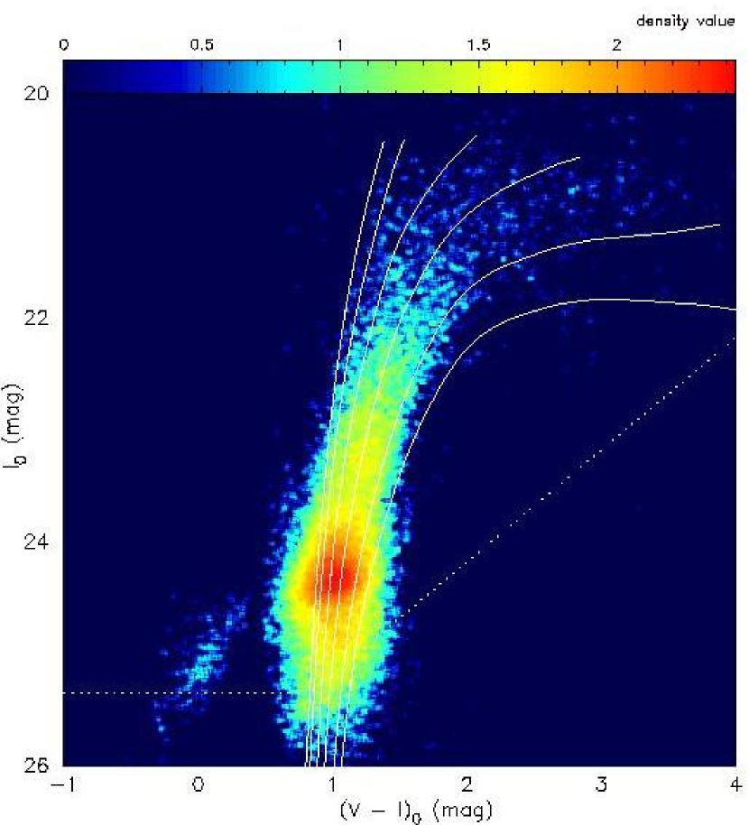
Figure 23.— A CMD in the $I_{0}$ vs. $(V-I)_{0}$ plane for stellar sources detected in the W-shelf field. The dotted lines denote the full range of the 50% completeness level. The superposed solid lines in the CMD show theoretical RGB tracks from VandenBerg et al. (2006) for an age of 12 Gyr, [$\alpha$/Fe]$=+0.3$, and metallicities (left to right) of [Fe/H]$=-2.31$, $-1.71$, $-1.14$, $-0.71$, $-0.30$ and $0.00$. The foreground/background contaminations have been subtracted based on the scaled control field of CompL103Bm16_5.

Figure 24.— Upper: Metallicity distribution functions (with error bars denoting Poisson uncertainties) for the W-shelf sample and the GSS sample, as interpolated from the chosen Victoria-Regina isochrones. The same photometric limits as Fig. 12 have been imposed. The control field, normalized with the gradient shown in Fig. 20, have been used to subtract the expected foreground/background counts in each of the metallicity bins. The dotted histogram is the same MD as the top-left histogram in the right-hand panel of Fig. 13. Lower: The cumulative MDs for the two substructures. The solid and dashed distributions appear very similar but the K-S statistics suggests that they are different.

5.2. South-East Streams C and D

Figure 25 shows close-up maps of the south-east minor-axis region in the proximity of our GSS field at $(\xi\sim 0.5,\eta\sim-2.2)$, divided [Fe/H] into two non-overlapping ranges ($+0.00$ to $-0.71$ and $-0.71$ to $-1.71$). This division for metallicities makes it clear that two overdense regions are indeed present, contrary to the expected smoothly declining stellar density of the halo. These overdense regions, which were first discovered by Ibata et al. (2007), are called Stream ‘D’ (at $\xi\sim 2.5,\eta\sim-1.8$) and ‘C’ (at $\xi\sim 3.5,\eta\sim-2.5$) in order of increasing declination. Actually, they are aligned in a direction perpendicular to the minor axis and more extending like a stream feature on both sides of our observed regions; we see only a part of the two streams.

Unfortunately these substructures show about $1/10$ lower surface brightness than the GSS and the W-shelf, and the detection limits for these data are somewhat worse than for the control field data. Thus, the method for subtracting the background contaminations in the CMD would need caution, when we simply compare with the control field having much better detection efficiency. Therefore, in Figure 26 we display the contamination-uncorrected CMDs of the stream-like structures within the range of projected $R\sim$ 50–60 (35–45) kpc for Stream C (Stream D). These CMDs are smoothed with a Gaussian kernel over 3 pixels ($d(V-I)=0.03,dI=0.03$) in order to diminish the effect of spiky noises attributable to low statistics. Here, as a further step, we have tried to roughly remove background galaxies in combination with a criterion based on the FWHM parameter derived from SExtractor (Bertin & Arnouts, 1996). The criterion was chosen along the stellar sequence in the space of magnitude vs. FWHM (e.g., Kashikawa et al., 2004). Since the detection method of sources in SExtractor suffers from blending objects, the detection limit gets into somewhat shallower in response to changes in worse seeing size. Nonetheless, both of the CMDs of Stream C and D as in Fig. 26 imposed by the stringent criterion present a clear RGB sequence along the theoretical isochrones at $I_{0}\lesssim 23.5$ and $(V-I)_{0}\sim 1$.

A prominent feature of the CMDs is that Stream C is predominantly metal-rich, being comprised of the stars in the range $-1.14<{\rm[Fe/H]}<-0.30$, while in Stream D metal-poor stars with the metallicity of $-1.71<{\rm[Fe/H]}<-0.71$ are well populated. The corresponding MDs of the two streams given in Figure 27 statistically confirm these features, where we have made the subtraction of contaminations as was done for the GSS and W-shelf fields. The mean metallicity with the standard deviation of Stream C (Stream D) is ${\rm[Fe/H]}=-0.89\pm 0.55$ ($-1.03\pm 0.61$) based on 1684 (1288) stars, assuming an age of 12 Gyr, [$\alpha$/Fe]$=+0.3$ and distance modulus of $24.43$ from Freedman & Madore (1990). The characteristics of this population difference are also suggested by the previous study based on the CFHT/MegaCam survey (Ibata et al., 2007); we have confirmed the existence of these faint outer streams based on our Subaru/Suprime-Cam data with higher S/N.

Now we further determine the mean age of the dominant populations based on the MD and RC magnitude. We present the luminosity functions of the Stream C and D in the expected magnitude range of the RC when assuming the aforementioned distance in Figure 28. The RC magnitudes of Stream C and D are $I_{0}=24.37$ and $24.47$, respectively. By determining a Gaussian peak as RC magnitude and convolving the MDs of Fig.27 with the magnitude, we estimate the mean ages of the dominant populations of these streams as $\sim 9.3^{+0.9}_{-1.4}$ Gyr for Stream C and $\sim 9.6^{+0.7}_{-1.1}$ Gyr for Stream D. The errors are based on the photometric errors, which strongly depend on the relation between RC magnitude and metallicity distribution at younger part as shown in Fig. 16.

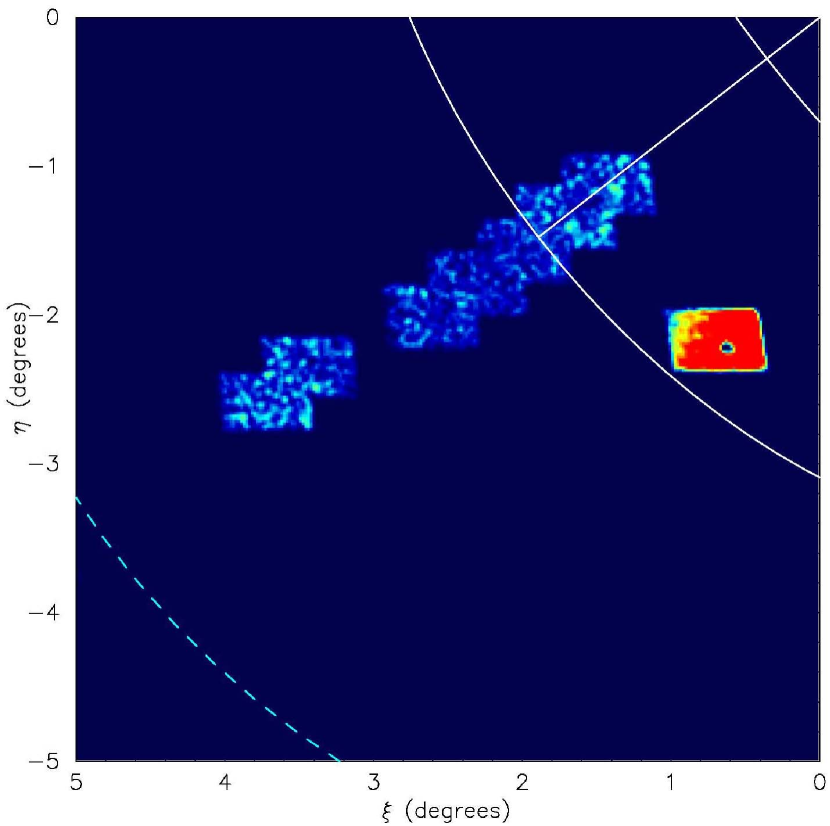
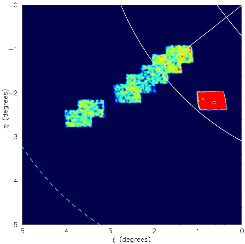
Figure 25.— The Stream C and D regions shown zoomed-in (from Fig. 21) with slices in [Fe/H] ($-0.71<{\rm[Fe/H]}<+0.00$ for left panel and $-1.71<{\rm[Fe/H]}<-0.71$ for right panel).

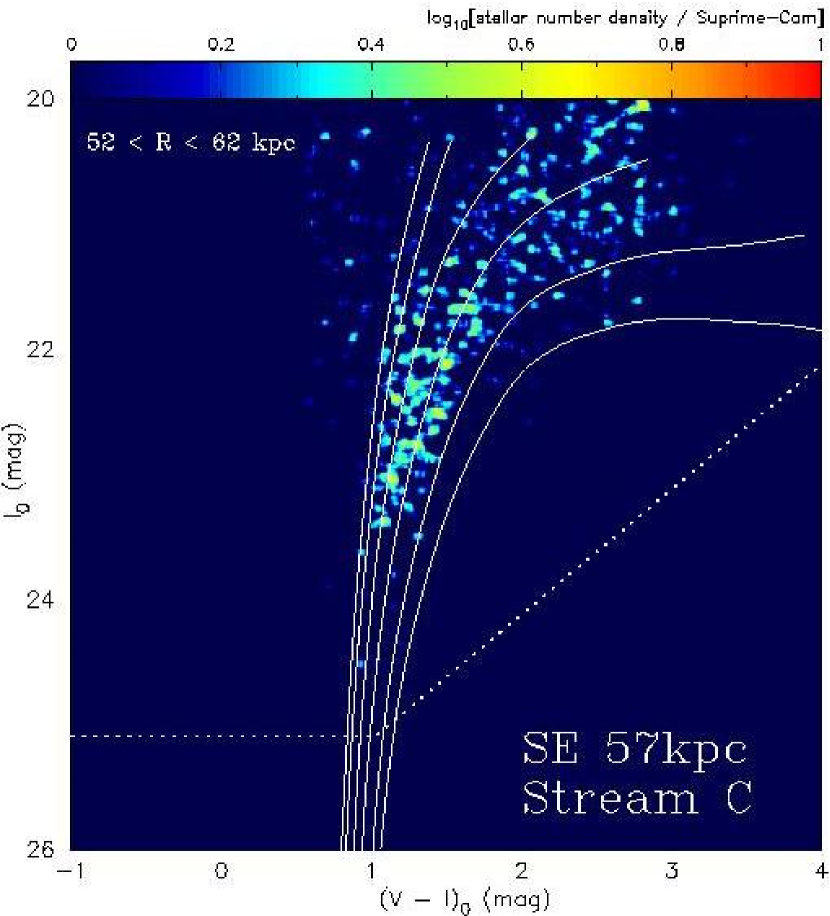
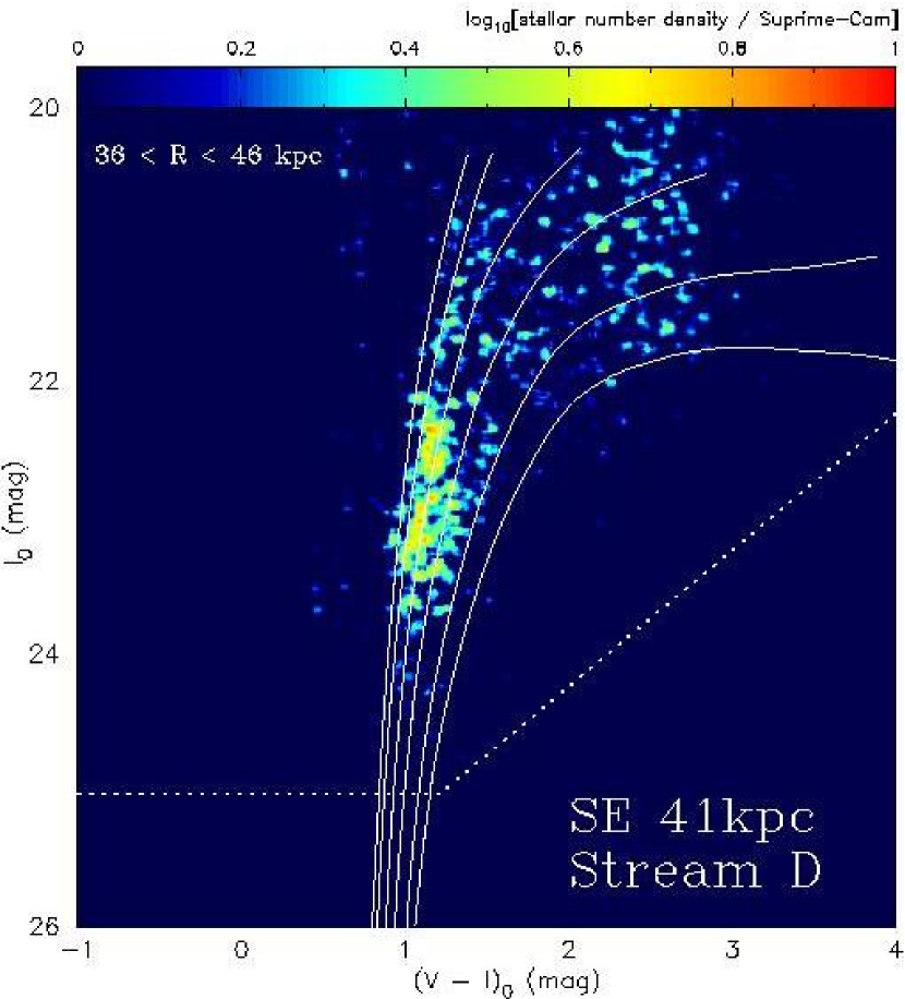
Figure 26.— Contamination-uncorrected CMDs for two adjacent Suprime-Cam fields along the south-east minor axis, evaluated with stringent criterion in SExtractor (see text). The superposed solid lines in the CMD show theoretical RGB tracks from VandenBerg et al. (2006) for an age of 12 Gyr, [$\alpha$/Fe]$=+0.3$, and metallicities (left to right) of [Fe/H]$=-2.31$, $-1.71$, $-1.14$, $-0.71$, $-0.30$ and $0.00$.

Figure 27.— MDs and cumulative MDs of the Stream C and D, using the Victoria-Regina theoretical isochrones for an age of 12 Gyr and [$\alpha$/Fe]$=+0.3$ (as shown in Fig. 26), on the assumption that these substructures are as old as a diffuse, classical halo.

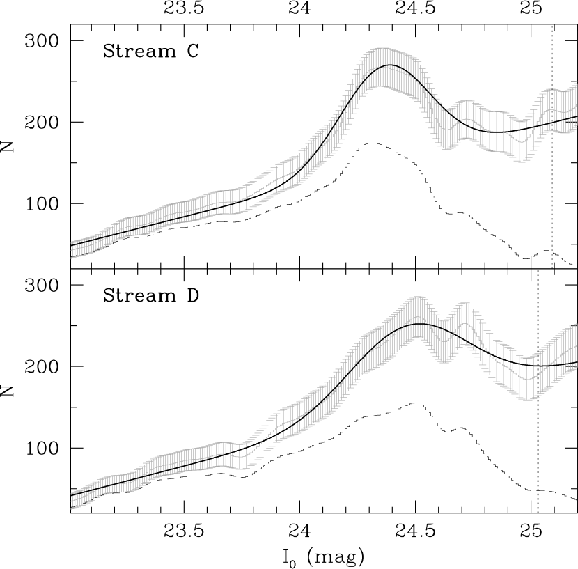
Figure 28.— Luminosity functions of the Stream C and D around the RC. Solid line is the completeness-corrected LF with Poisson uncertainties, while the dotted line is the completeness-uncorrected LF. Red line is the best-fitted model with a simple model consisting of a Gaussian plus a straight line. We determine a Gaussian peak as the magnitude of the RC. Vertical dotted line denotes the 50% completeness limit.

5.3. Major-Axis Structure

The faint diffuse structure extended along the south-west major axis between a projected distance of 50 and 100 kpc was mentioned in Ibata et al. (2007). Although our Suprime-Cam survey regions are slightly different from those covered by CFHT/MegaCam and both of the two surveys do not encompass the entire region of the diffuse major-axis structure, the CMD of these areas shows a clearly well-populated metal-poor RGB sequence with a dominant population in the metallicity range of $-2.31<{\rm[Fe/H]}<-1.14$ (Figure 29). The corresponding MD and cumulative MD using about 420 stars and the Victoria-Regina theoretical isochrones for an age of 12 Gyr and [$\alpha$/Fe]$=+0.3$ are displayed in Figure 30. They are constructed by imposing further color criterion with $(V-I)_{0}<1.8$ in order to avoid the heavy foreground disk dwarf contamination, considering the existence of the dominantly populated metal-poor stars as shown in the CMD. The mean metallicity of the population is ${\rm[Fe/H]}\sim-1.2$. Our confirmed stellar population in the diffuse structure on the south-west major-axis is in nice agreement with that of Ibata et al. (2007), and there is no population gradient of the diffuse structure in both of the survey fields.

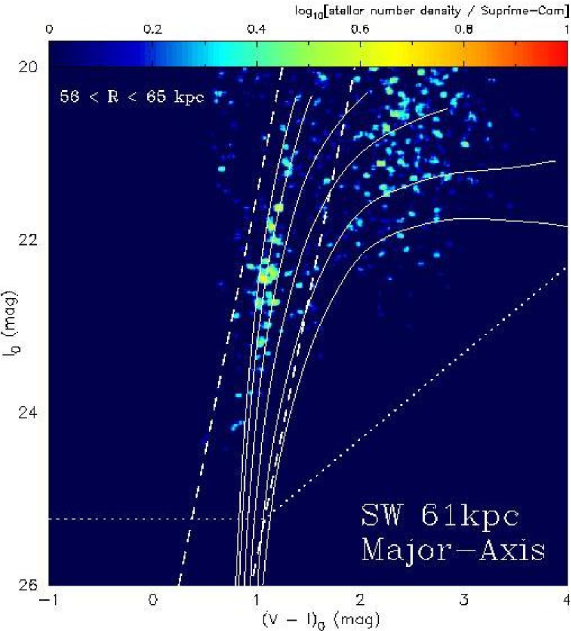
Figure 29.— Contamination-uncorrected CMD of the major-axis diffuse population, evaluated after stringent criterion in SExtractor (see text).

Figure 30.— The MD and the cumulative MD of the major-axis diffuse structure, using the Victoria-Regina theoretical isochrones for an age of 12 Gyr and [$\alpha$/Fe]$=+0.3$. We also select a bluer sample with $(V-I)_{0}<1.8$ to avoid the heavy contamination of disk dwarfs.

Ibata et al. (2007) concluded that the two stellar populations of the diffuse structure and the GSS are different and likely unrelated despite the visual impression that the density map of their Figure 21 gives indications that the major-axis population merges with the GSS. However, in the LF shown in Figure 31, we detect a subtle peak similar to the RC over Poisson noise, suggesting that there is an intermediate-age population in the diffuse halo structure. If the peak morphology with $I_{0}=24.34$ is actually attributable to the RC, we can estimate the mean age of the population as $\sim 8.6^{+0.9}_{-1.5}$ Gyr. This estimation provides a comparable age to the GSS. Based on their numerical simulation, Fardal et al. (2008) actually reproduced the decline in the mean metallicity from the central core of the GSS to its cocoon to the southwest, using an accretion model of a disk-like progenitor having a strong radial metallicity gradient. Thus, this may suggest that the metal-poor/young population of the diffuse halo structure originated from the debris of the GSS’s progenitor. So we cannot readily rule out the association of the diffuse structure with the GSS. A much deeper and wider survey reaching down to the main-sequence turn-off by a planned thirty meter telescope is necessary to more accurately determine the age and the distance to the diffuse structure. Additionally the spectroscopic survey to measure kinematics will be needed to understand the origin of these halo structures in detail.

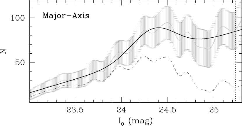
Figure 31.— Luminosity functions of the major-axis diffuse structure around the RC.

5.4. New North-West Streams E and F

Here, we report on two new substructures seen in the north-west portion of the outer halo of M31. In contrast to the south quadrant of M31’s halo which has been studied by a few other groups, the north quadrant has remained unexplored until now, in part because its low Galactic latitude ($b\sim-10^{\circ}$) results in a high degree of contamination by foreground Milky Way dwarf stars.

The two overdense structures on the north-west minor axis at $R\sim 60$ and 100 kpc can be deduced from the visual inspection of the matched filter maps in Figure 32. This figure shows close-up maps of the north-west minor-axis region, divided by [Fe/H] into two non-overlapping ranges ($+0.00$ to $-0.71$ and $-0.71$ to $-1.71$). Here, we refer to these as Stream E and F, corresponding to the inner 60 kpc and outer 100 kpc substructures in the discussion below. Their dominant RGB population has a metallicity range of $-2.31<{\rm[Fe/H]}<-0.71$ in the Victoria-Regina isochrones, as can be seen in Figure 33. Although the data of Stream E were obtained under the worst conditions in our observing run, we can confirm well-populated metal-poor stars near the bright end of the M31 RGB. This population has a very similar CMD and surface brightness to those of the major-axis diffuse structure discussed in § 5.3. It also follows that Stream F shows a clear metal-poor RGB with a narrow metallicity range, as shown in the right panel of Fig. 33. This population has a very similar CMD to that of faint Stream A located at $R\sim 120$ kpc along the south-east minor axis as found by Ibata et al. (2007).

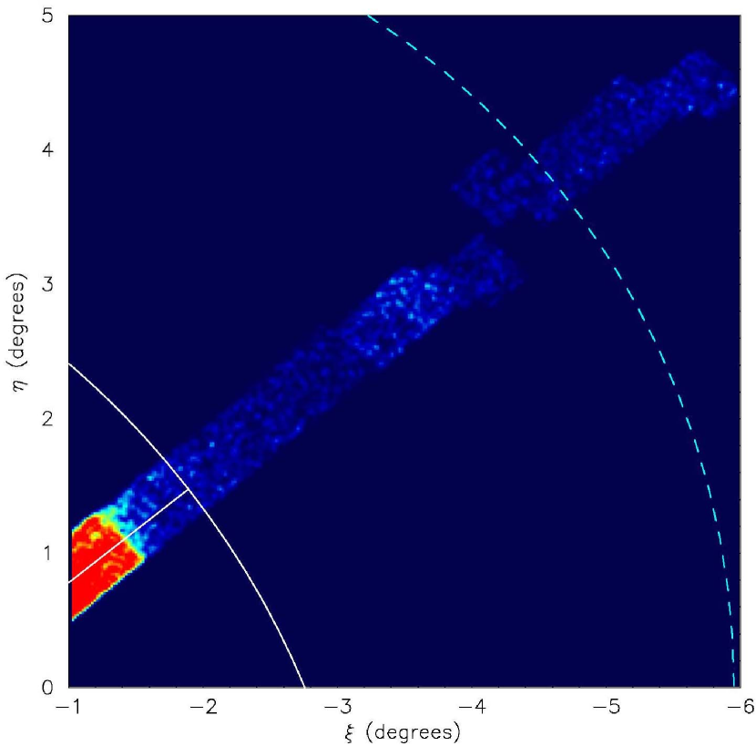
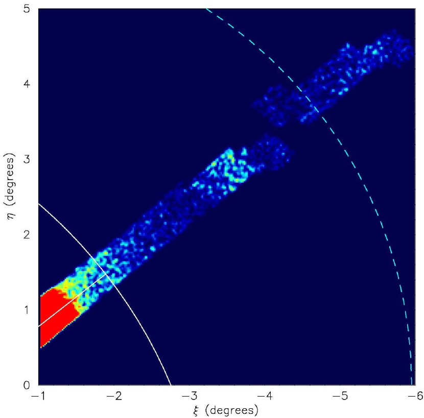
Figure 32.— The Stream E and F region shown zoomed-in (from Fig. 21) with slices in metallicities ($-0.71<{\rm[Fe/H]}<+0.00$ for left panel and $-1.71<{\rm[Fe/H]}<-0.71$ for right panel).

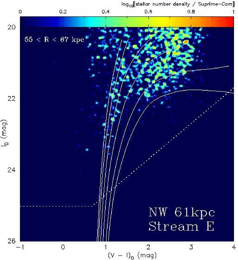
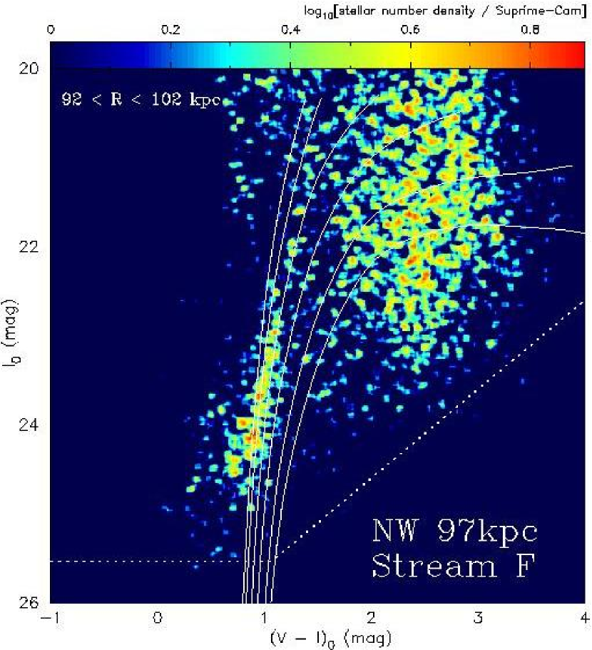
Figure 33.— The CMDs of Stream E and F, as derived in the same manner as Fig. 26. The CMD of Stream E is made of combined catalog from 55 to 67 kpc, while the one of Stream F is constructed by summed-up catalogs from 92 to 105 kpc. The superposed solid lines in the CMD show theoretical RGB tracks from VandenBerg et al. (2006) for an age of 12 Gyr, [$\alpha$/Fe]$=+0.3$, and metallicities (left to right) of [Fe/H]$=-2.31$, $-1.71$, $-1.14$, $-0.71$, $-0.30$ and $0.00$.

The MDs corresponding to these two newly-found streams are shown in Figure 34, where we use the Victoria-Regina theoretical isochrones for an age of 12 Gyr and [$\alpha$/Fe]$=+0.3$. In the north region of the M31 halo, the number of Galactic dwarf stars exponentially increases as shown in Fig. 20, while the stellar density of the M31 halo exponentially decreases with increasing radius (e.g., Gilbert et al., 2006). Therefore, because of the large uncertainty in correcting the disk contamination and the low statistics in extracting the intrinsic population of the M31 halo, we further impose the additional criterion of $(V-I)_{0}<1.8$ to construct the MDs, as was done for the MD of the major-axis structure (Fig. 30). The properties of the MDs clearly confirm the visual inspection of the above-discussed CMDs. Note that in this procedure we may miss some amount of the metal-rich stars with [Fe/H] $\gtrsim-0.7$ because of this stringent criterion.

Figure 34.— Metallicity distribution function and the cumulative distribution of the Stream E and F, statistically constructed in the same manner as the MD of the major-axis diffuse structure.

6. The Global Halo Properties Along the Minor Axis

6.1. Population Variation with Increasing Radius

In Figures 35 and 36 we display the CMDs along the minor axis in order of projected distance from the M31 center. After the background contaminations in the catalogs are subtracted by combination of DAOPHOT and SExtractor softwares in the same manner as our example above, we merge each catalog into final catalogs covered in 0.8–1.6 times field-of-views of a Suprime-Cam field and normalize them in the instrumental sky coverage with $34\arcmin\times 27\arcmin$. It appears that the number density of the foreground Galactic disk dwarf stars predictably increases with decreasing galactic latitude, that is, in the northern direction from the M31 center and the number density of Galactic halo stars is practically constant along these galactic latitudes within the Poisson noise. This suggests that our method for the separation of galaxies and stars works successfully at the brighter magnitude. In contrast, at the fainter magnitude of, for instance, $I_{0}\gtrsim 23.5$ $(I_{0}\gtrsim 23)$ for the SE 27kpc (41kpc) CMD, stellar objects seem to be over-subtracted because of the rapidly declining detection efficiency based on the above-mentioned stringent criterion.

The two CMDs among the four south-east CMDs show the stream-like substructures (Stream C and D) as shown in § 5.2. The inner most CMD at SE 27 kpc has wide-spread RGB stars and it is very similar to that of the north-west counterpart field (NW 28 kpc), suggesting the existence of complex mix of metal-rich and metal-poor populations with $-2.5\lesssim{\rm[Fe/H]}\lesssim 0.0$ in the inner halo of M31. Both of the populations in the two symmetrically-located fields have the same mean metallicity of ${\rm[Fe/H]_{\rm mean}}\sim-1.0$. A KS test of the two cumulative MDs imposed by the additional criterion with $(V-I)_{0}<1.8$ (mag) in order to avoid the foreground contamination yields a probability of 12.3% that the two distributions are drawn from the same parent distribution.

In our Suprime-Cam survey of the M31 halo, we have obtained data of continuous fields along the north-west minor axis, facilitating the investigation of global halo structure. Furthermore, most regions in the north-west halo have yet been unexplored by any other telescopes. The continuous change of the CMDs along the north-west minor axis of Figure 36 suggests the existence of clear population gradients with distance from M31’s center. The fraction of the metal-rich population with ${\rm[Fe/H]}\gtrsim-0.7$ strongly decreases out to $\sim 50$ kpc in projection, while the metal-poor stars with ${\rm[Fe/H]}\lesssim-0.7$ are definitely distributed in the outer part of $\sim 50$ kpc from the M31 center. This population variation identified from the CMDs reflects a strong metallicity gradient with increasing radius in the M31 halo. In the more remote halo beyond $\sim 50$ kpc, the RGB sequence with any metallicity range is virtually unobservable, except in the two overdense regions such as Stream E and F fields.

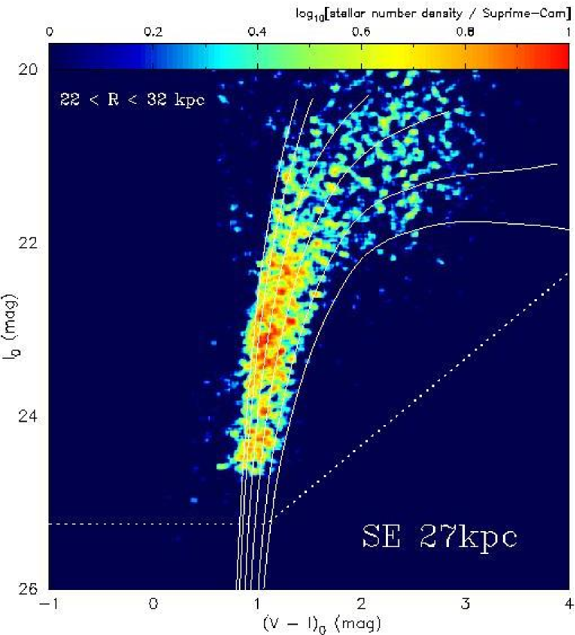
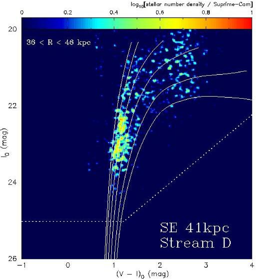
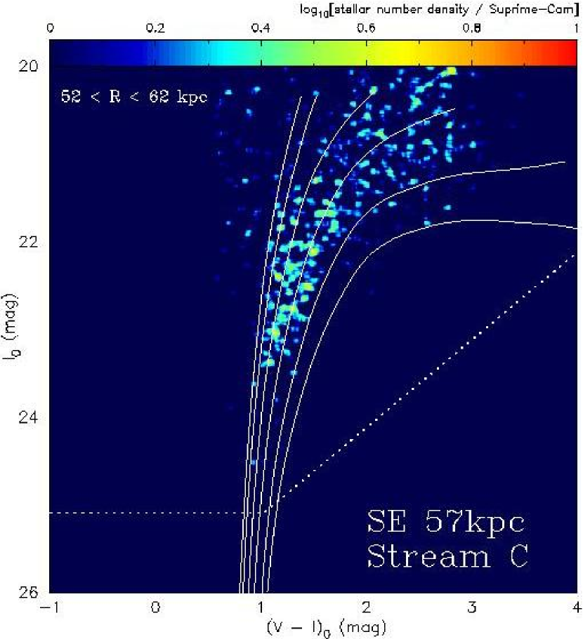
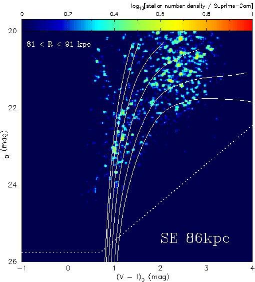
Figure 35.— The CMDs along the south-east minor axis of the M31 halo. The superposed solid lines in the CMD show theoretical RGB tracks from VandenBerg et al. (2006) for an age of 12 Gyr, [$\alpha$/Fe]$=+0.3$, and metallicities (left to right) of [Fe/H]$=-2.31$, $-1.71$, $-1.14$, $-0.71$, $-0.30$ and $0.00$.

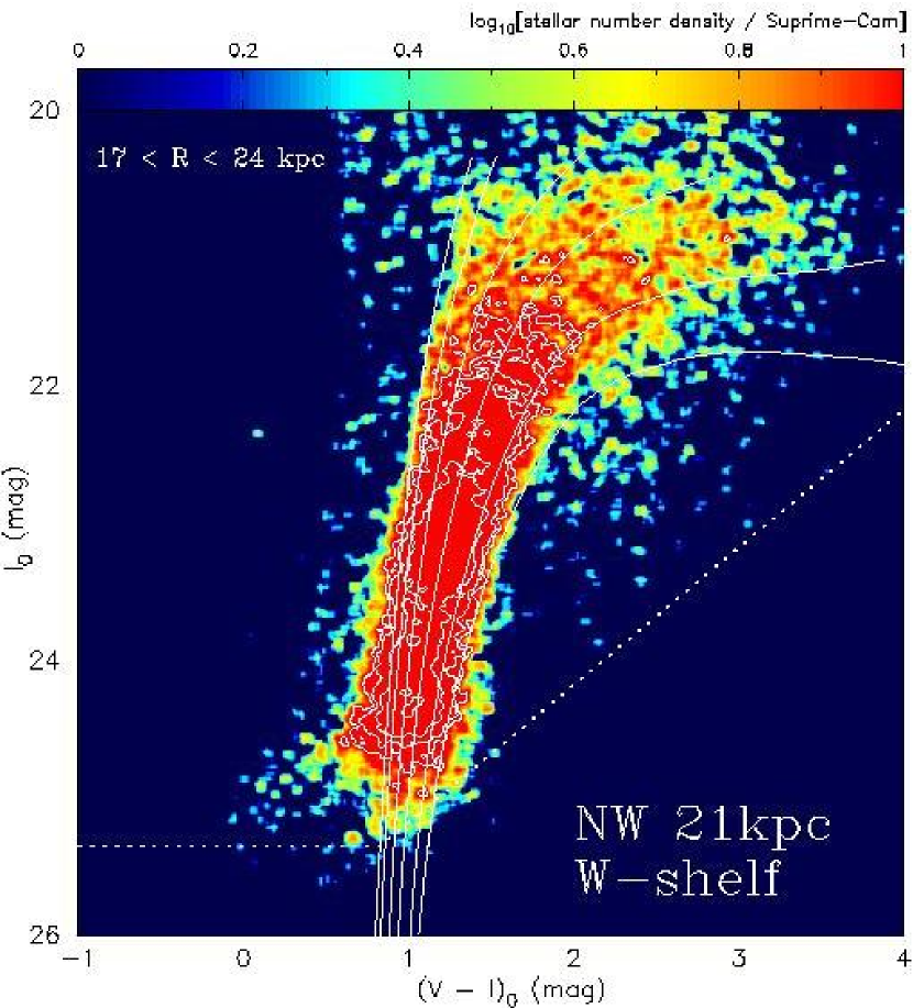
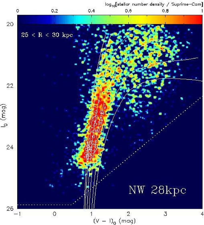
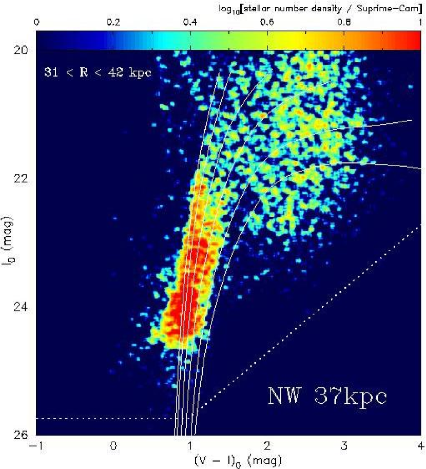
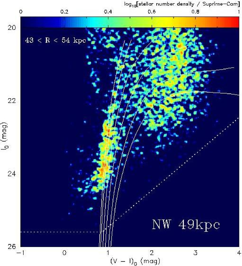
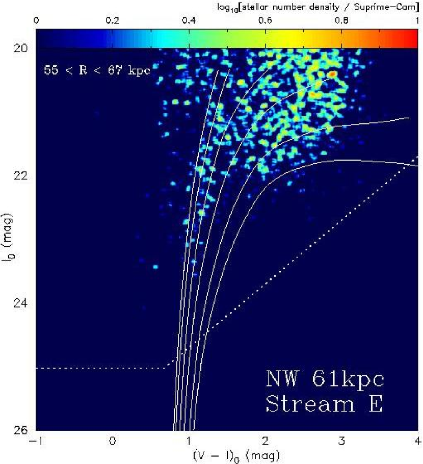
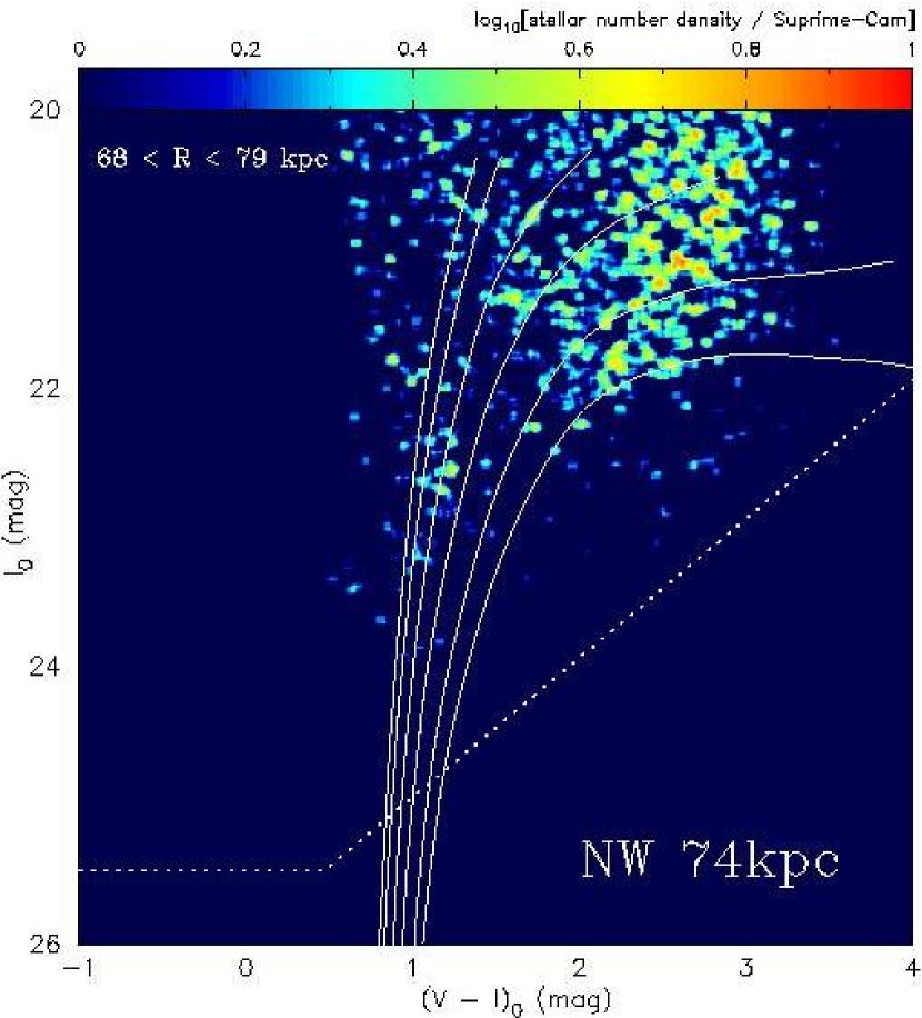
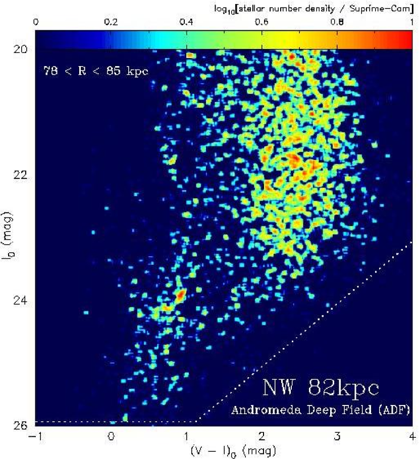
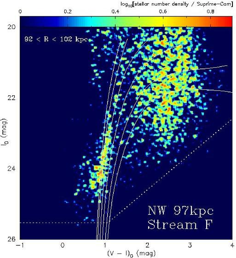
Figure 36.— The CMDs along the north-west minor axis of the M31 halo. The superposed solid lines in the CMD show theoretical RGB tracks from VandenBerg et al. (2006) for an age of 12 Gyr, [$\alpha$/Fe]$=+0.3$, and metallicities (left to right) of [Fe/H]$=-2.31$, $-1.71$, $-1.14$, $-0.71$, $-0.30$ and $0.00$.

6.2. Surface Brightness Profiles

Since Pritchet & van den Bergh (1994) derived the surface brightness (SB) profile of the inner dense parts of the M31 spheroid, many researchers have studied the extended, outer parts of the halo along the south-east minor axis (Durrell et al., 2004; Irwin et al., 2005; Guhathakurta et al., 2005; Ibata et al., 2007). In contrast to the inner parts of the spheroid, it is possible to resolve the individual stars in its outer parts, because of their sparse density and of the sufficiently close distance of M31 to us. Thus the SB profiles in the spheroid’s outer parts are available by directly counting individual stars. While previous studies have been limited to relatively bright RGB stars for the estimation of the SB in an extended halo, we consider fainter stars, taking advantage of the light-gathering power of the Subaru telescope with an 8.2-m primary mirror. This suggests that the results obtained here using our deep Suprime-Cam data will be most robust against the effects of any contaminations over the fields. Furthermore, considering both the north-west and the south-east halo profiles simultaneously for the first time, we will arrive at more comprehensive halo structures than have been studied previously.

We estimate the SB profiles using the RGB and AGB stars selected as $(V_{0},~{}I_{0})<(24.8,~{}24.0)$, i.e., $I$-band magnitude brighter than the Red Clump (at $I_{0}\sim 24.5$) and colors redder than $(V-I)_{0}=0.8$, with not less than about 90% completeness limit. In addition we set $I_{0}\gtrsim 20.3$, i.e., fainter than the tip of RGB stars of M31 (e.g., Durrell et al., 2001), to exclude contaminations such as foreground stars, when assuming the distance modulus of 24.43 from Freedman & Madore (1990).

First, we divide a series of our surveyed fields shown in Fig. 1 into subregions with about $0.05$ square degrees. After extracting the secure RGB stars based on the above magnitude and color selection criteria, we divide them into the following two groups using the RGB model isochrones of VandenBerg et al. (2006) for an age of 12 Gyr and [$\alpha$/Fe]$=+0.3$: Metal-Poor group (MP) defined as $-2.31<{\rm[Fe/H]}<-0.71$ and Metal-Rich group (MR) defined as $-0.71<{\rm[Fe/H]}<+0.00$. This division is motivated by the form of the CMDs as obtained above (§ 6.1), showing a rather distinct feature below and above [Fe/H]$\sim-0.7$ (corresponding to the metallicity of one of the Galactic clusters, 47 Tuc (catalog )).

Second, we convert the summed-up flux counts of selected stars to the SB in mag arcsec^-2, and subtract the SB of the control field, for which foreground and background contaminants are removed based on the statistical method outlined in § 2.3.2. The sources of noise in this method of estimating the SB arise from the Poisson statistics from the finite number of observed stars and subtracted contaminations.

Figure 37 shows the reduced SB profiles of the MP (blue) and MR (red) groups. In this figure, two colored dotted lines having flat profiles present the subtracted background levels to obtain the reduced SB profiles. In addition, we plot the SB in our observed regions of the GSS and the major-axis diffuse structures (green and grey). The top panel of the figure denotes the SB profiles selected by our color cut of $(V-I)_{0}<4.0$ used in the construction of the MDs in the previous sections, whereas the bottom panel shows the SB profiles chosen by the bluer color cut of $(V-I)_{0}<1.8$ used in the construction of the MDs of the above-discussed outer streams. The latter color cut is motivated to avoid the heavy contamination of the disk dwarf stars. For guidance, a dashed line corresponds to the SB profile obtained by Ibata et al. (2007), based on their survey for south outer parts of the halo; they identified stream-like substructures in some parts of our observed fields, whereby they derived the SB profile for the global halo by avoiding such disturbing substructures. This line is characterized by a power-law model, $\Sigma(R)\varpropto R^{-\alpha}$, with an exponent of $\alpha=1.91\pm 0.12$ kpc. We nominally fit this SB profile to our fields at $R\sim 30$ kpc, which may lie outside the inner dense spheroid with a $R^{1/4}$ law and trace an extended halo just beyond this component. It follows that this SB profile reproduces this inner part of an extended halo. At the brighter part of $\mu_{V}\lesssim 33$ mag arcsec^-2, the decreasing trend of the estimated SBs in both the north-east and south-west parts is reasonably consistent with each other. We are also able to assess the faint stream-like substructures as identified in the population maps of Fig. 21. However, the absolute SB given in a dashed line is slightly underestimated in the inner region, which is dominated by metal-rich stars such as the W-shelf field. In contrast, at the fainter part of $\mu_{V}\gtrsim 33$ mag arcsec^-2, in particular, in the north-west region, the behavior of the SB profiles are somewhat different. As discussed in § 6.1, it is supposed that we do not detect both metal-rich and metal-poor stars in the outer region of $R\gtrsim 80$ kpc because we could not identify the metal-rich RGB with ${\rm[Fe/H]}>-0.7$ on the CMDs (see Fig. 36). Therefore, in the outer halo regions beyond $R\sim 80$ kpc we accept the SB profiles based on the more stringent color criterion of $(V-I)_{0}<1.8$, compared to those with $(V-I)_{0}<4.0$. Then, a prominent feature of interest is that the number of metal-rich stars with ${\rm[Fe/H]}\gtrsim-0.7$ in the north-west halo of M31 steeply decreases with increasing radius, compared to the south-east halo, because the south-east region within $R\sim 70$ kpc may be polluted by substructures with metal-rich populations such as Stream C, D and the diffuse debris of the GSS as predicted by Fardal et al. (2007). This picture is slightly inconsistent with our assumption that the region along the south-east minor axis at $R\sim 35$ kpc is free from any substructures, so we used the region for the control field through the analysis of the GSS in § 3. However, we note that the effect of such substructures does not significantly change the final result of our analysis for the GSS because the number of the contaminated metal-rich stars at the $R\sim 35$ kpc field is only a small percent of those in our observed field of the GSS as shown in the right panel of Fig. 37.

To investigate the spatial distribution of the M31 halo in more detail, we attempt to fit the data on the radial profile (by weighting the Poisson errors in the star counts) of four theoretical models of the surface density profile. The power-law and exponential models have been used to reproduce the surface brightness of some stellar systems (e.g., Binney & Tremaine, 1987). The NFW and Hernquist models representing the (dark matter) density profile are derived from Navarro et al. (1996) (converted into the projected formula by Bartelmann 1996) and Hernquist (1990), respectively; this model choice is motivated by the simulations of Bullock & Johnston (2005). The dashed lines in Figure 38 show four different model fits to the selected minor axis regions, which are selected to probe a smooth, dynamically relaxed halo, where the contamination by substructures appears small. The inner halo, which may hold complex structures mixed by the debris of the GSS and/or the edge of the W-shelf structure, provides the upper limit to the radial SB profile of the minor-axis halo.

Indeed, the outer halo profile appears remarkably flat in log-linear representation, thereby indicating essentially an exponential function. The black dashed line in Fig. 38 shows an exponential model fit to the data of MP group; we find a large exponential scale length of $R_{h}=18.8\pm 1.8$ ($22.4\pm 2.3$) kpc for north-west (south-east) minor axis halo. We also show a projected Hernquist model fit (thin short-dashed line) to these data; the best model gives a scale radius of $R_{h}=17.1\pm 4.7$ ($31.7\pm 6.7$) kpc, suggesting that the scale radius for north-west halo is comparable to that of Bullock & Johnston (2005) while that for the south-east halo is about a factor of 2 larger than predicted by Bullock & Johnston (2005). Ibata et al. (2007) also indicates the flat density distribution as well as our south-east result, based on more outer and wider regions in the south quadrant halo out to 140 kpc, because our south-east fields from 20 to 90 kpc are polluted by many substructures such as Stream B, C and D.

These results, in particular for the north-west profile, are of great importance for understanding the nature of M31’s halo, so these are to be assessed from a more careful analysis. We know that the number counts of background galaxies rapidly increases in the fainter magnitude range as shown in Kashikawa et al. (2004). Therefore, there is concern about the misclassification of background galaxies on the above calculated SB profiles. To test this effect, we re-calculate the SB profile along the north-west regions as before for the selected metallicity range, but this time we adopt an additional selection of stars: we further limit the halo sample with higher S/N, by imposing more stringent color-magnitude criteria of $(V_{0},~{}I_{0})<(24.3,~{}23.5)$. The results are shown in Figure 39. It is evident that these plots are qualitatively and quantitatively identical to those based on the previous selection using deeper data. Also shown is the predicted behavior of the Galactic foreground contamination (with the same color-magnitude selection) as a dotted line in the figure. This profile of the contamination is nearly flat in this log-linear representation, so contamination cannot account for the observed profile. Thus, this smooth decline for the outer halo population of M31, which is comparable to the density profile predicted by the Bullock & Johnston (2005) model, is a robust result of this survey. We note that the density profile of the north-west minor axis halo derived here is steeper than that of the south-east minor axis halo derived by Ibata et al. (2007). This is because their sample is shallower than ours and they have underestimated the surface brightness in the denser, inner regions of the halo.

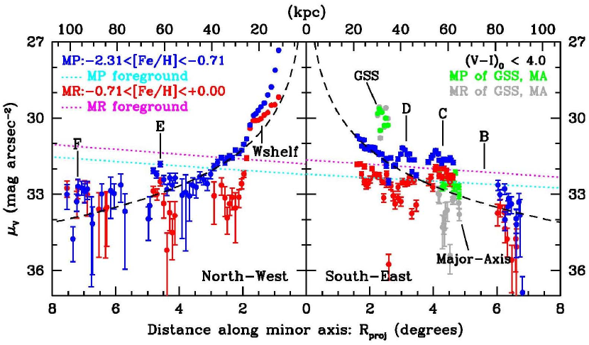
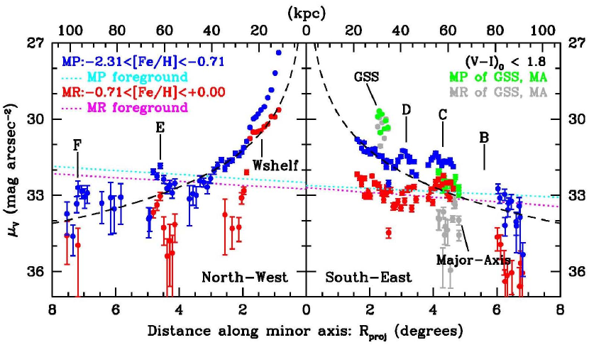
Figure 37.— The minor-axis profiles for RGB stars as derived from the MP and MR group, which are illustrated with blue and red points, respectively. Dotted lines denote the corresponding subtracted background levels. The error bars reflect a combination of Poisson statistics and background uncertainties. The dashed line shows a power-law profile with an exponent of $1.91\pm 0.12$ for MP group derived by Ibata et al. (2007), for the sake of comparison. The distinction between the upper and lower panels reflects different color selection (see text).

Figure 38.— The north-west (south-east) minor-axis radial profile from the MP group is shown in upper (lower) panel. We reject the data containing the overdense regions as we have shown in the text. The thick long-dashed line is a power-law fit to these data with $\alpha=2.17\pm 0.15$ $(1.75\pm 0.13)$, while the thick short-dashed line is an exponential profile with scale length of $R_{h}=18.8\pm 1.8$ $(22.4\pm 2.3)$ kpc. The thin short-dashed line shows the best-fit Hernquist model, which has a scale length of $R_{h}=17.1\pm 4.7$ $(31.7\pm 6.7)$ kpc. In addition, with the thin long-dashed line, we show the NFW model for the halo mass profile with a scale length of $R_{h}=0.2\pm 3.5$ $(6.3\pm 3.9)$ kpc.

Figure 39.— Same as the upper panel of Fig. 38, but for stars restricted in the small color-magnitude region $V_{0}<24.3$ and $I_{0}<23.5$, in order to more stringently remove the heavy background contamination. Thus, these plots are only for the purpose of verifying the effects of such contamination on the derived surface brightness profile. The thick long-dashed line is a power-law fit to these data with $\alpha=1.95\pm 0.18$, while the thick short-dashed line is an exponential profile with scale length of $R_{h}=19.5\pm 2.3$ kpc. The thin short-dashed line shows the best-fit Hernquist model, which has a scale length of $R_{h}=24.1\pm 7.0$ kpc. In addition, with the thin long-dashed line, we show the NFW model halo mass profile with a scale length of $R_{h}=2.6\pm 4.5$ kpc.

6.3. Metallicity Distributions

We derive the spatial variation of mean/median metallicities along the minor-axis of M31’s halo, by comparing the RGB stars on the CMD of each halo field to theoretical isochrones from VandenBerg et al. (2006) in the same manner as previous constructions of the MDs. For adopted theoretical isochrones we assume the old and $\alpha$-enhanced populations with an age of 12 Gyr and [$\alpha$/Fe]$=+0.3$ like the Milky Way halo. Regarding our current method for the estimation of metallicities using these old isochrones, it is noted that recent studies by Brown et al. (2003, 2006b) suggest an intermediate age, i.e., younger than 10 Gyr, for about one third of the inner halo stars, in contrast to the Galactic halo population. More recent studies with HST/ACS (Brown et al., 2007, 2008) have revealed the existence of truly ancient and metal-poor populations as well as younger populations in the inner halo of M31. While the age of these halo populations is yet to be fully understood, our method using the old theoretical isochrones provides appropriate lower limits on the metallicities of stars. However, as discussed in § 3.3.1, for low-mass RGB stars with ages of 6-14 Gyr the metallicity derived from interpolation/extrapolation of bright RGB stars hardly depends on such an age difference (Kalirai et al., 2006b).

We show their mean (median) metallicities as a function of distance from the M31 center in the upper (lower) panel of Figure 40. Several black filled circles present the average values of mean/median metallicities in our targeted fields, while numerous black open circles are those in the subfields, which are obtained by dividing a continuous field into the subfields with about $0.05$ square degrees. These subfields help us to examine a fine spatial variation inside a single Suprime-Cam field. Conversely, each filled black filled circle reflects the mean value of metallicities for the subfields. Vertical error bars of the upper (lower) panel show the associated standard deviation (interquartile interval) of the mean (median) metallicities.

These plots suggest that the stellar content of the M31 halo has no metallicity gradient within our observed range of fields. However, the spatial variation from 20 to 50 kpc along the north-west minor axis appears to have a slight metallicity gradient. Our analysis of the CMDs discussed in § 6.1 robustly confirms the presence of the gradient. However, while the CMD analysis also predicts the lack of metal-rich stars in the more remote outer region, the figure shows the unexpected high fraction of metal-rich stars at $R\gtrsim 80$ kpc. This is because the derived mean/median metallicities in the outer halo are somewhat overestimated due to the heavy contamination of the Galactic disk dwarf stars as discussed in § 6.2. Therefore, we re-calculate the mean/median metallicities by imposing a more stringent color cut of $(V-I)_{0}<1.8$, to ensure a minimal contamination from the Galactic disk. The results are shown in Figure 41. The mean/median metallicities in the south-east region show a systematic decrease of about 0.2 dex while keeping no spatial gradient. In contrast, the variation in the north-west region based on the stringent color criterion shows now a strong metallicity gradient.

We further test whether this strong metallicity gradient is a real feature or not, in addition to the above-confirmed morphological variation in the CMD along the north-west minor-axis. Figure 42 denotes the ratio of the signal-to-noise (S/N) ratio, plotted as a function of north-west minor-axis distance from the M31 center (in projection), where the S/N ratio means the ratio of the number of objects used to calculate the mean/median metallicity in each summed-up field to the number of the foreground sources in the scaled control field. The vertical axis of Fig. 42 means the ratio of the S/N ratio of $(V-I)_{0}<1.8$ selection sample to the signal-to-noise ratio of $(V-I)_{0}<4.0$ selection. Basically, because the vertical value is more than 1.0 in most regions of the north-west halo, the spatial variation of mean/median metallicities based on the stringent color criterion of $(V-I)_{0}<1.8$ is statistically more reliable than that based on a $(V-I)_{0}<4.0$ color cut. However, note that the absolute mean/median metallicities are clearly somewhat underestimated in the inner fields with a lot of metal-rich stars at $R\lesssim 40$ kpc along the north-west minor axis. Eventually, we conclude that this test provides the lower limit to the radial metallicity gradient photometrically detected in the north-west minor axis halo.

Figure 40.— Upper panel shows the mean metallicity of north-west (left) and south-east (right) halo regions together with the associated standard deviation, plotted as a function of distance from the M31 center (in projection), while lower panel presents the median one together with the associated interquartile interval. Filled black circles present the average values of mean/median metallicity in the targeted fields, while black open circles denote those in each divided subfield (see text). Gray filled and open triangles present the mean/median metallicities of summed-up and individual fields of the major-axis diffuse structure, respectively.

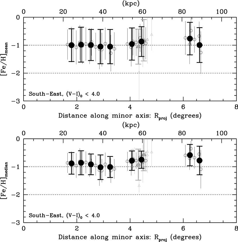
Figure 41.— Same as Fig. 40, but for stars restricted to the small color region $0.9<(V-I)_{0}<1.8$, to ensure a minimal contamination from the Galactic disk.

Figure 42.— The comparison of the two S/N ratios, (S/N)_1.8 [with a color cut of $(V-I)_{0}<1.8$] and (S/N)_4.0 [with $(V-I)_{0}<4.0$], plotted as a function of north-west minor-axis distance from the M31 center (in projection), where the S/N ratio means the ratio of the number of the residual objects used to calculate the mean/median metallicity in each summed-up field to the number of the foreground sources in the scaled control field.

7. Discussion

7.1. The Distribution of the Underlying Halo

In this study, one of our major purposes is to clarify the general properties of the underlying, smooth halo component of M31. As mentioned in § 1, recent large-scale photometric and spectroscopic surveys of the M31 halo have revealed the existence of the metal-poor and old populations (like a classical smooth halo in the Milky Way), which are buried in the inner complex metal-rich and young substructures (e.g., Kalirai et al., 2006b; Ibata et al., 2007). By the term “smooth”, what we mean here is not necessarily that the component is perfectly spatially smooth, but instead that any substructures that may be present in the halo are below detectability with the current survey.

The surface brightness profile as shown in § 6.2 is a good indicator to describe the radial extent of the halo. Since many studies of the density distributions of the Milky Way halo have already been made, it is useful to compare such results with our current studies of the M31 halo. The Milky Way halo has been characterized by a steep power-law density profile $\rho(r)\propto r^{-\gamma}$: its power-law index, $\gamma$, is in the range of $2.5$ to $3.6$. Some of the variance in the value of $\gamma$ appear among different research groups, which can be attributed to the presence of substructures in the halo; previous studies have commonly been limited in sky coverage, so some local structures in the halo can affect a final result. Surveys covering significant portions of the sky have been feasible only recently. For instance, the most recent SDSS study by Jurić et al. (2008), which made use of good distance estimates to halo stars near main-sequence turnoff covering 6500 deg² of sky, found $\rho(r)\propto r^{-2.8}$ corresponding to $\alpha=1.8$ as a power-law index of the surface brightness profile. Similarly, Bell et al. (2008) have found the stellar density distribution with $\rho(r)\propto r^{-3}$, based on about $4\times 10^{6}$ color-selected main-sequence turnoff stars contained in the SDSS DR5 catalog. Although in these SDSS surveys accurate investigations of the density profile are limited only within $R\sim 20$ kpc (or at most 40 kpc, relied on the QUEST RR Lyrae sample of Vivas & Zinn 2006) due to the uncertainty in the determination of the distance to remote stars, these results for the Milky Way halo are completely consistent with the present result of the M31 halo, $\Sigma(R)\propto R^{-2.17\pm 0.15}$ (i.e., $\gamma\sim 3.2$), as derived for the north-west minor-axis halo out to $R\sim 100$ kpc.

It is worthwhile to compare our current result of the radial profile of the M31 halo with other observational studies dedicated to the outer halo. Our photometrically-estimated north-west profile is in reasonably agreement with the south-east profile of $\Sigma(R)\propto R^{-1.91\pm 0.12}$ based on the large south quadrant area out to 140 kpc (in projection) from the M31 center by the photometric CFHT/MegaCam survey of Ibata et al. (2007). In contrast, our result is slightly flatter than Guhathakurta et al. (2005) and Gilbert et al. (2006) who have found an extended stellar halo in M31 following $\Sigma(R)\propto R^{-2.6}$ (or $R^{-2.3}$) out to $R\sim 165$ kpc, based on the kinematically-selected RGB sample by the Keck/DEIMOS observation. However, we note that the former authors have not removed unresolved background galaxies which significantly affect fields under the worse seeing condition as discussed in § 2.3.2 and their survey is more than one magnitude shallower than our Suprime-Cam survey. The latter authors have estimated the radial profile of the M31 halo derived from secure spectroscopic RGB sample in the remote outer halo, but it is based on only $\sim 40$ red giants to determine the outer profile beyond $R=60$ kpc.

Recent numerical simulations predict that most of the mass in the stellar halo originates in satellites that were accreted more than 8 Gyr ago (corresponding to at $z\simeq 1$). The halo is smoothly built from the inside out within the finite dynamical time scale, and becomes the dominant contributor at 30–60 kpc and within (Bullock & Johnston, 2005; Abadi et al., 2006). Our derived surface density profile of the M31 halo in the external view is in excellently agreement with the density profile of the accreted stellar halo; it is described as a Hernquist profile with $R_{h}\simeq 14$ kpc within the radial range dominated by the ancient halo, as expected by the Bullock & Johnston (2005) model. In the meantime, our NFW fitting based on the observed SB profile returns several times higher concentration value ($c\equiv R_{\rm vir}/R_{h}$) than that derived from the simulations based on dark matter distributions (e.g., Bullock & Johnston, 2005), assuming the typical virial radius (e.g., $R_{\rm vir}=200$ kpc) of Milky Way-type galaxies. This fact suggests that the visible baryonic matter like stars may well converge in the galactic center compared to the invisible dark matter because of baryon dissipation during accretion processes.

7.2. Implications for the Origin of Substructures

Another major purpose of the current study is to probe the origin of various substructures as found in both the inner and outer parts of the M31 halo. Their metallicity distributions as well as the spatial distributions of substructures are useful information to untangle the formation history of the halo because each substructure preserves such fossil records associated with star formation and merging/accretion events.

7.2.1 The South-East Minor Axis Substructures

As shown in the previous subsection, the spatial distribution of mean/median metallicity along the south-east minor axis of the M31 halo remains approximately constant with increasing radius from the center. This is because our observing fields with Suprime-Cam coincidentally overlap some overdense stream-like substructures, characterized by Stream D, C and B of Ibata et al. (2007), which dominate the metallicity distribution of the stars in these fields. Stream D and C have similar high mean metallicity but clearly different CMD morphology and metallicity distributions as shown in § 5.2, suggesting that these two populations are different. Stream B brushes our outermost south-east field at $R\sim 90$ kpc, as shown in the south quadrant map of Ibata et al. (2007). This constancy in the mean metallicity variation is consistent with the prediction by many previous studies, proposing that the halo is built-up through the dissipationless chaotic assembly from small subgalactic fragments (e.g., Searle & Zinn, 1978).

However, the absence of metallicity gradient conflicts with the result of Kalirai et al. (2006b) and Koch et al. (2007), who found a strong metallicity gradient in the south-east minor axis discrete fields out to $\sim 165$ kpc, based on the kinematically-selected RGB sample with the Keck/DEIMOS spectrograph. The mean metallicities in the Subaru fields (SE2 and SE9) which overlap with the two fields studied in Kalirai et al. (2006b) (their a0[30kpc] and m6[87kpc]) are actually almost consistent with those given in their paper ($\langle$[Fe/H]$\rangle\sim 1.1$), although their work showed a metallicity gradient over larger radii out to $R\sim 165$ kpc. On the other hand, some discrepancies with the Koch et al. (2007) result are puzzling. These authors re-analyzed the same data as Kalirai et al. (2006b) but using a different method for metallicity determination and found a strong metallicity gradient, where the metallicity at $R\sim 90$ kpc is [Fe/H]$=-2.4$, i.e., more metal-poor than our result of [Fe/H]$\sim-1$. Although comprehensive understanding of this descrepancy is difficult only from our photometric studies, Stream B which distributes over our fields at $R\sim 90$ kpc may affect the determination of a global metallicity distribution, as mentioned above. To settle this issue, it is necessary to carry out a wider-field photometric/spectroscopic survey over the large outer part of the M31 halo.

In addition, we compare with the main-sequence fitting results based on the HST/ACS deep observations of Brown et al. (2008) who found the trend that the mean age becomes simply older beyond 30 kpc in the south-east inner region. In fact, we have found that at 27 kpc, 41 kpc (corresponding to Stream D), and 57 kpc (corresponding to Stream C), the mean ages are $\sim 10$, $\sim 9.6$, and $\sim 9.3$ Gyr, respectively, as derived from their MDs and RC magnitudes using the theoretically-computed relation of Rejkuba et al. (2005) (see Fig. 16). These results suggest that there exist some inhomogeneities of the halo, which is yet on the way to the equilibrium structure.

7.2.2 The North-West Minor Axis Substructures

The mean metallicity variation along the north-west minor axis, based on continuous Suprime-Cam pointings out to $\sim 100$ kpc, shows a strong spatial gradient with increasing radius. This is consistent with the result of Kalirai et al. (2006b) and Koch et al. (2007). This spatial dependence of abundance distribution may conflict with the scenario of galactic halo formation via hierarchical merging, where successive merging events can erase any spatial gradients in metallicities as confirmed by numerical simulations. For instance, the study of Font et al. (2006b) predicts a gradient in [Fe/H] averaged over each full simulated halo of at most 0.5 dex over a few tens of kpc.

It is yet difficult to clarify the physical origin of the detected metallicity gradient in the halo because there exist few observations and simulations for the presence of a strong abundance gradient with increasing radius in the halo. A possible explanation for the current result is that the observed spatial distribution of metallicities may reflect just a snapshot of the dynamical evolution, which is on the way to the equilibrium structure characterized by a flatter metallicity gradient. In particular, the halo structure is dominated by transient substructures, which may largely affect the spatial distribution of metallicities instantaneously. Indeed, modern galaxy formation simulations within the context of the standard $\Lambda$CDM cosmology predict that the outer halo beyond $R\sim 50$ kpc is dominated by numerous faint arcs, shells and streams, as the relaxation time of these subsystems as found at large distances from the galaxy center is quite long at such locations, where even the dynamical time is of order of Gyr (e.g., Bullock & Johnston, 2005; Johnston et al., 2008). Furthermore, dynamical friction is at work, which acts more strongly on more massive subhalos, making them fall rapidly into the potential well, where they become disrupted and their contents are mixed into the evolving galaxy. We then observe a rather steep metallicity gradient just after this event occurs.

7.2.3 Dispersed Faint Substructure?

Satellites with sufficiently long accretion times of more than several Gyr would contribute to the wide range of the stellar halo, so it is difficult to find any density substructures in such well-mixed systems at the present day. It is noteworthy that previous studies found kinematically cold substructures based on the detailed Keck/DEIMOS spectroscopic observations in the south regions of the M31 halo, where no evidence for the presence of substructures has been deduced from photometric observations (Kalirai et al., 2006a; Gilbert et al., 2007; Chapman et al., 2008). These results suggest the possibility that there are also as-yet unrelaxed debris from disrupted dwarf satellites underneath the smooth halo at the north-west 30-40 kpc fields. Some $N$-body simulations (e.g., Bekki & Chiba, 2001) predicted that these optically faint substructures below our detected surface brightness levels may still exist in phase space, kinematics. In this regard, we discuss about the possibility of the existence of these dispersed faint substructures in this subsection.

As long as the surface brightness profiles (Fig. 37 and 38) are concerned, there is no evidence for overdense substructures in the north-west and south-east regions at 30 kpc. However, we find the age difference between both fields; the mean age of the stellar population in the north-west part ($\sim 7.5\pm 1.5$ Gyr) is about 2.5 Gyr younger than that in the south-east counterpart field ($\sim 10\pm 1$ Gyr), as derived from their MDs and RC magnitudes using the theoretically-computed relation of Rejkuba et al. (2005) (see Fig. 16). In fact, we cannot insist that the two populations originated from the same stellar population because the KS probability for this hypothesis based on their two cumulative MDs is rather low. Therefore, we expect that there might be a dispersed faint substructure in the seemingly smooth regions at $R=$ 30–50 kpc in the north-west minor axis halo, which preserves the information of ancient accretion events. In addition, note that the age difference could be occurred by the difference in the distance of the same population substructures. To distinguish these much fainter substructures from the smooth inner halo we need additional kinematic studies as well as some abundance information (such as $\alpha$-element abundance) as predicted in Johnston et al. (2008).

Suppose that in the north-west region of M31 halo there exists such a well-mixed substructure with sufficient long accretion time (e.g., 9 Gyr), it may be possible to trace this accretion event from our photometric data if the event provides some specific stellar populations. If so, we expect a specific magnitude of the RC/AGBb feature, where a clustered distribution of stars in color-magnitude diagrams allows us to easily identify the presence of such stellar populations, compared to attempts to detect faint spatial substructures from already smeared out surface density distribution. Also we can estimate the mass of an accreted satellite as $\sim 1\times 10^{9}M_{\sun}$, which corresponds to ${\rm[Fe/H]_{\rm mean}\sim-1.0}$. Then, if we suppose that this progenitor galaxy genuinely has an intermediate-age population, it is likely that such a galaxy possibly having interstellar gas has undergone a star formation driven by, for instance, the second or third collision or supernova wind about 7.5 Gyr ago.

7.2.4 Comparison with Recent Numerical Simulations

The recent models also predict that substructures that we can discover in the remote outer halo more likely have low surface brightness compared to the inner substructures with high metallicity and high surface brightness (e.g., Bullock & Johnston, 2005; Johnston et al., 2008). In particular, Johnston et al. (2008) predict that in a stellar halo of Milky Way type galaxies being built entirely from accretion within a $\Lambda$CDM context, the fraction of the system (of the order of 10% of its stars) are comprised of distinct substructures, i.e., a few to a dozen streams which are brighter than 35 mag arcsec^-2 at projected distances greater than 30 kpc from the host galaxy. Figure 43 shows the same cumulative distribution derived from our M31 observations and Ibata et al. (2007): the GSS, Stream A to F and the major-axis diffuse structure. The gray zone indicates plausible upper and lower limits, if simply extrapolated to the entire survey region. It is evident that both luminosity functions derived from the models and the observations are reasonably similar, suggesting that the outer halo of M31 as well as the Milky Way halo has been built up by recent accretion events of satellite galaxies. Furthermore, Figure 44 plots the average metallicity against SB for these substructures including our W-shelf data. Gray circles show the Stream A and B substructures of Ibata et al. (2007). Since metallicity uncertainties are just roughly plotted based on the error analysis in § 3.3.1, in practice they may be slightly larger. Despite this, we find that higher SB tidal debris tend to be more metal-rich, which is confirmed by some recent numerical simulations (e.g., Font et al., 2008; Johnston et al., 2008). This result implies that higher SB debris may tend to come from the more luminous, metal-rich dwarf satellites and/or recent encounters. However, while more detailed theoretical approaches to the issue are required, it is also of great importance to explore more and fainter substructures in the larger region of the M31 halo using the next-generation wide-field imager such as Hyper Suprime-Cam, to set tighter limits on the halo formation history.

It is worth noting that recent high-resolution $N$-body simulation made by Mori & Rich (2008) provides an interesting scenario for the M31 halo: a merging event of a dwarf satellite into the halo of M31 gives rise to an elongated substructure similar to the GSS, the giant stellar stream found in the south-east part of M31’s halo. Also, their model suggests that further stream-like substructures emerge in the form of concentric shells around a galaxy after collisions with a disk component and subsequent relaxation process, and that a multiple large-scale shell system is finally formed in the outer region of the halo; the outermost large-scale shells have a radius of $>50$ kpc and survive for at least 4 Gyr. If this is the case, then widely-separated shell structures would appear in the form of concentric shells around M31’s halo. Although with this anticipation it is difficult to understand the existence of the clearly different radial metallicity gradients found along the north and south parts of M31, we actually have been able to identify two overdense substructures at the north-west counterpart fields. Considering their CMD morphology, it appears that the counterpart of Stream E is Stream B and that of Stream F is Stream A, although there is some positional shift of about 15–20 kpc. Since it is not yet clear that these counterpart streams indeed have the same populations, we need to carry out further observations of the M31 halo with a wider and deeper imaging survey, in order to clarify the detailed stellar population and the true spatial extension of these substructures.

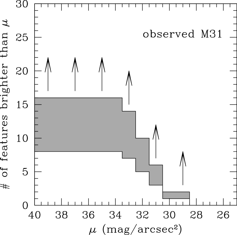
Figure 43.— The cumulative number of distinct substructures observed in the M31 halo, based on our work and Ibata et al. (2007). The gray zone indicates plausible upper and lower limits, if simply extrapolated to the entire survey region.

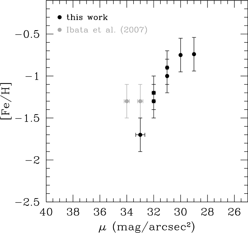
Figure 44.— The average metallicity against SB for the substructures combining our M31 observations and Ibata et al. (2007) (see text). Metallicity uncertainties ($\pm 0.2$ dex) are roughly plotted based on the error analysis in § 3.3.1. Higher SB tidal debris tend to be more metal-rich.

8. Conclusions

We have investigated the structure and stellar populations of the stellar halo in the Andromeda galaxy, using deep and wide-field $V$ and $I$-band images taken with Subaru/Suprime-Cam. From the analysis of the CMDs through comparing isochrones and globular cluster fiducials, the fundamental properties of each halo structure identified here have been derived, such as distance, surface brightness profiles, metallicities and ages of the stellar populations. Our results for each of the GSS and other halo structures (substructures and smooth halo) are summarized as follows.

8.1. The Andromeda Giant Stream

We have identified an intermediate-age and metal-rich RC population as well as a broad RGB sequence in the Andromeda GSS. From the $VI$ CMD and the LF, we have measured the distance to our observed stream field of $(m-M)_{0}=24.73\pm 0.11$ ($883\pm 45$ kpc) based on the $I$-magnitude of the TRGB and reddening $E(B-V)=0.05$. This result supports the previous prediction of McConnachie et al. (2003) that their Field 5 ($840\pm 20$ kpc) which falls near GSS1 is at about 100 kpc further away along the line of sight relative to M31’s main body.

From the photometric comparison of more than 7000 bright RGB stars in our stream field with the RGB templates of Galactic globular clusters, we have obtained the metallicity ditributions (MDs) of the GSS for a statistically significant sample. It shows the characteristics summarized as the peak metallicity of [Fe/H]${}_{\rm peak}\hskip 3.00003pt\raisebox{1.72218pt}{$>$}\raisebox{-3.01385pt}{$\sim$}\hskip 3.00003pt-0.5$, the average metallicity of [Fe/H]${}_{\rm mean}=-0.6$ and the median metallicity of [Fe/H]${}_{\rm med}=-0.5$. This result is in excellent agreement with that of kinematically selected RGB stars in the same stream field (Guhathakurta et al., 2006). Furthermore, based on the stellar mass/luminosity-metallicity relation observed for the Local Group dwarf galaxies shown in Côté et al. (2000) and Dekel & Woo (2003), the mass of the plausible progenitor is in the range of $10^{7}$ to $10^{9}M_{\sun}$, which is consistent with the work of Mori & Rich (2008).

The feature near RC, showing an extended brighter part relative to its peak, is an unambiguous signature of an intermediate age population, which is also supported by the existence of an AGB bump. We have estimated the age of the stellar population in the GSS, by convolving the MDs and the RC magnitudes with the theoretical models from Rejkuba et al. (2005). As a result, we have found that the dominated population of the GSS has the mean age of $\sim 8$ Gyr, consistent with the main-sequence fitting results with the HST/ACS observations by Brown et al. (2006b).

The GSS possibly originated from the accretion or minor merger of a massive dwarf satellite within the mass range of $10^{7}$ to $10^{9}M_{\sun}$, like M32, but previous studies suggests that M32 itself is probably not a progenitor of the GSS, as we already mentioned in Section 1. Considering the finite dynamical time of such a mass accretion, the progenitor has to be bound to M31 several billion years ago as judged from the current residual substructure. The first pericentric merging may well induce the third star forming event from the remaining gas, whereas 30% of the GSS stars were provided in this event.

8.2. The Andromeda Stellar Halo

Our method for analyzing the CMDs of the GSS has also been applied to other large survey regions of the M31 halo. Main results obtained from the outer halo survey are summarized as follows:

• In the outer halo beyond $R\sim 30$ kpc, M31 contains a multitude of overdense substructures compared to the smooth radial profile, such as streams, arc and shells. We confirm the two substructures, namely Stream C and D, discovered by Ibata et al. (2007). Furthermore, from our constructed stellar density maps we have found two as-yet unknown overdense substructures in the north-west halo, which we call Stream E and F in this work. It is yet unclear to what extent these substructures are spatially distributed.

• We have derived the fundamental properties of these four stream-like structures in addition to the major-axis diffuse structure implied by Ibata et al. (2007) and the Western shelf seen in the star count map of Ferguson et al. (2002). The derived properties are summarized in Table 5. We have found that higher SB tidal debris tend to be more metal-rich, which is confirmed by some recent numerical simulations (e.g., Font et al., 2008; Johnston et al., 2008). This result implies that higher SB debris may tend to come from the more luminous, metal-rich dwarf satellites and/or recent encounters.

• By separating regions showing obvious substructures, we have found that the remaining area of the survey exhibits a smooth metal-poor stellar halo component in the north-west minor axis halo. This structure needs not to be perfectly spatially smooth, but the intrinsic inhomogeneities are below the sensitivity of this study. The smooth halo is vast, extending out to the radial limit of the survey, at $R=100$ kpc. The SB profile of this component can be modeled with a Hernquist profile as suggested by simulations, and the resulting scale radius of $\sim 17$ kpc is comparable to what modern halo formation simulations predict. A power-law profile with $\Sigma(R)\propto R^{-2.17\pm 0.15}$ [$\rho(r)\propto r^{-3.17\pm 0.15}$] can also be fitted to the data. Our NFW fitting based on the observed SB profile returns a several times higher concentration value than that derived from the simulations based on dark matter distributions (e.g., Bullock & Johnston, 2005), assuming the typical virial radius (e.g., $R_{\rm vir}=200$ kpc) of Milky Way-type galaxies. This fact suggests that the visible baryonic matter may well converge into the galactic center compared to the invisible dark matter because of energy dissipation in the course of accretion process.

• We have detected metallicity inhomogeneities in different radial directions. The spatial distribution of mean metallicity along the south-east minor axis of the M31 halo remains approximately constant, while that along the north-west minor axis shows a strong spatial gradient with $R$ out to 100 kpc. This fact suggests that the halo may be yet in the course of the dynamical evolution, leading subsequently to a flatter metallicity gradient.

In conclusion, the outer halo of the Andromeda galaxy as well as that of the Milky Way can be formed from distinct stellar substructures deposited from over $\sim 15$ independent accretion events of subhalos with masses similar to typical dwarf galaxies, i.e., of order $10^{7}$–$10^{9}M_{\sun}$. The Andromeda galaxy has quietly undergone the accretion of these intermediate-mass subhalos without the destruction of the disk (e.g., Kazantzidis et al., 2008) since $z\sim 1$ corresponding to $\sim 8$ Gyr ago. However, in the stellar halo of M31 there are probably much fainter substructures below detectability with the current survey, as suggested by the existence of further relaxed substructures (e.g., slightly younger substructures discussed in § 7.2) and kinematic substructures recently discovered in some spectroscopic studies (Kalirai et al., 2006a; Gilbert et al., 2007; Chapman et al., 2008). Therefore, we will need further observations with higher sensitivity to arrive at a better understanding of the formation of M31’s stellar halo.

Table 5Fundamental properties of the substructures

Name	Distance	$\mu_{V}$(typical)	$\langle$[Fe/H]$\rangle$	$\langle$age$\rangle$	Progenitor mass
(Projected Distance from M31)	kpc	mag arcsec-2	dex	Gyr	$M_{\sun}$
Giant Stream ($\sim 30$ kpc)	$883\pm 45$	$\hskip 3.00003pt\raisebox{1.72218pt}{$<$}\raisebox{-3.01385pt}{$\sim$}\hskip 3.00003pt29$	$-0.74$	$\sim 8$	$\sim 10^{9}$
W-shelf ($\hskip 3.00003pt\raisebox{1.72218pt}{$<$}\raisebox{-3.01385pt}{$\sim$}\hskip 3.00003pt25$ kpc)	$798\pm 40$	$\sim 30$	$-0.75$	$\sim 8$	$\sim 10^{9}$
Stream D ($\sim 35$-45 kpc)	–	$\sim 31$	$\sim-1.0$	$\sim 10$	$\sim 10^{9}$
Stream C ($\sim 50$-60 kpc)	–	$\sim 31$	$\sim-0.9$	$\sim 9$	$\sim 10^{9}$
MA structure ($\sim 60$ kpc)	–	$\sim 32$	$\sim-1.2$	$\sim 9$?	$\sim 10^{8}$
Stream E ($\sim 60$ kpc)	–	$\sim 32$	$\sim-1.3$	–	$\sim 10^{8}$
Stream F ($\sim 100$ kpc)	–	$\sim 33$	$\sim-1.7$	old?	$\sim 10^{7}$

References

- Abadi et al. (2006) Abadi, M., Navarro, J., & Steinmetz, M. 2006, MNRAS, 365, 747
- Alves & Sarajedini (1999) Alves, D. R., & Sarajedini, A. 1999, ApJ, 511, 225
- Bartelmann (1996) Bartelmann, M. 1996, A&A, 313, 697
- Bekki & Chiba (2001) Bekki, K., & Chiba, M. 2001, ApJ, 558, 666
- Bell et al. (2008) Bell, E. F., et al. 2008, ApJ, 680, 295
- Bellazzini et al. (2002) Bellazzini, M., et al. 2002, AJ, 123, 1509
- Bellazzini et al. (2003) Bellazzini, M., et al. 2003, A&A, 405, 867
- Bertin & Arnouts (1996) Bertin, E., & Arnouts, S. 1996, A&AS, 117, 393
- Binney & Tremaine (1987) Binney, J., & Tremaine, S. 1987, Galactic Dynamics (Princeton: Princeton Univ. Press), 747
- Brown et al. (2003) Brown, T. M., et al. 2003, ApJ, 592, L17
- Brown et al. (2004) Brown, T. M., et al. 2004, ApJ, 613, L125
- Brown et al. (2006a) Brown, T. M., et al. 2006a, ApJ, 636, L89
- Brown et al. (2006b) Brown, T. M., et al. 2006b, ApJ, 652, 323
- Brown et al. (2007) Brown, T. M., et al. 2007, ApJ, 658, L95
- Brown et al. (2008) Brown, T. M., et al. 2008, ApJ, 685, L121
- Bullock & Johnston (2005) Bullock, J. S., & Johnston, K. V. 2005, ApJ, 635, 931
- Carretta & Gratton (1997) Carretta, E. & Gratton, R. 1997, A&AS, 121, 95
- Carretta et al. (2001) Carretta, E., et al. 2001, AJ, 122, 1469
- Chapman et al. (2006) Chapman, S. C., et al. 2006, ApJ, 653, 255
- Chapman et al. (2008) Chapman, S. C., et al. 2008, MNRAS, 390, 1437
- Choi et al. (2002) Choi, P. I., Guhathakurta, P., & Johnston, K. V. 2002, AJ, 124, 310
- Côté et al. (2000) Côté, P., et al. 2000, ApJ, 533, 869
- Couture et al. (1995) Couture, J., et al. 1995, AJ, 109, 2050
- Dean et al. (1978) Dean, J. F., Warren, P. R., & Cousins, A. W. J. 1978, MNRAS, 183, 569
- Dekel & Woo (2003) Dekel, A., & Woo, J. 2003, MNRAS, 344, 1131
- Durrell et al. (2001) Durrell, P. R., Harris, W. E., & Pritchet, C. J. 2001, AJ, 121, 2557
- Durrell et al. (2004) Durrell, P. R., Harris, W. E., & Pritchet, C. J. 2004, AJ, 128, 260
- Fardal et al. (2006) Fardal, M. A., et al. 2006, MNRAS, 366, 1012
- Fardal et al. (2007) Fardal, M. A., et al. 2007, MNRAS, 380, 15
- Fardal et al. (2008) Fardal, M. A., et al. 2008, ApJ, 682, L33
- Ferguson et al. (2002) Ferguson, A. M. N., et al. 2002, AJ, 124, 1452
- Ferguson et al. (2005) Ferguson, A. M. N., et al. 2005, ApJ, 622, L109
- Ferrarese et al. (2000) Ferrarese, L. et al. 2000, ApJS, 128, 431
- Ferraro et al. (2000) Ferraro, F.R. et al. 2000, AJ, 119, 1282
- Font et al. (2006a) Font, A. S., et al. 2006a, AJ, 131, 1436
- Font et al. (2006b) Font, A. S., et al. 2006b, ApJ, 646, 886
- Font et al. (2008) Font, A. S., et al. 2008, ApJ, 673, 215
- Ferrarese et al. (2000) Ferrarese, L., et al. 2000, ApJS, 128, 431
- Freedman & Madore (1990) Freedman, W. L., & Madore, B. F. 1990, ApJ, 365, 186
- Gallart (1998) Gallart, C. 1998, ApJ, 495, L43
- Gilbert et al. (2006) Gilbert, K. M., et al. 2006, ApJ, 652, 1188
- Gilbert et al. (2007) Gilbert, K. M., et al. 2007, ApJ, 668, 245
- Girardi et al. (2000) Girardi, L., et al. 2000, A&AS, 141, 371
- Girardi et al. (2002) Girardi, L., et al. 2002, A&A, 391, 195
- Guhathakurta et al. (2005) Guhathakurta, P., et al. 2005, astro-ph/0502366
- Guhathakurta et al. (2006) Guhathakurta, P., et al. 2006, AJ, 131, 2497
- Hernquist (1990) Hernquist, L. 1990, ApJ, 356, 359
- Holland et al. (1996) Holland, S., Fahlman, G. G., & Richer, H. B. 1996, AJ, 112, 1035
- Ibata et al. (2001) Ibata, R. A., et al. 2001, Nature, 412, 49
- Ibata et al. (2004) Ibata, R. A., et al. 2004, MNRAS, 351, 117
- Ibata et al. (2007) Ibata, R., et al. 2007, ApJ, 671, 1591
- Irwin et al. (2005) Irwin, M., et al. 2005, ApJ, 628, L105
- Iye et al. (2004) Iye, M., et al. 2004, PASJ, 54, 833
- Johnston et al. (2008) Johnston, K. V., et al. 2008, ApJ, 689, 936
- Jurić et al. (2008) Jurić, M., et al. 2008, ApJ, 673, 864
- Kalirai et al. (2006a) Kalirai, J. S., et al. 2006a, ApJ, 641, 268
- Kalirai et al. (2006b) Kalirai, J. S., et al. 2006b, ApJ, 648, 389
- Kashikawa et al. (2004) Kashikawa, N., et al. 2004, PASJ, 56, 1011
- Kazantzidis et al. (2008) Kazantzidis, S., et al. 2008, ApJ, 688, 254
- Koch et al. (2007) Koch, A., et al. 2008, ApJ, 689, 958
- Landolt (1992) Landolt, Arlo U. 1992, AJ, 104, 340
- Lee et al. (1993) Lee, M. G., Freedman, W. L., & Madore, B. F. 1993, ApJ, 417, 553
- Madore & Freedman (1995) Madore, B. F., & Freedman, W. L. 1995, AJ, 109, 1645
- Majewski et al. (2000) Majewski, S. R., et al. 2000, AJ, 120, 2550
- Martin et al. (2007) Martin, N., Ibata, R., & Irwin, M. 2007, ApJ, 668, L123
- McConnachie et al. (2003) McConnachie, A. W., et al. 2003, MNRAS, 343, 1335
- McConnachie et al. (2004) McConnachie, A. W., et al. 2004, MNRAS, 351, L94
- Miyazaki et al. (2002) Miyazaki, S., et al. 2002, PASJ, 54, 833
- Mori & Rich (2008) Mori, M., & Rich, R. M. 2008, ApJ, 674, L77
- Morrison (1993) Morrison, H. L. 1993, AJ, 106, 578
- Mould & Kristian (1986) Mould, J., Kristian, J. 1986, ApJ, 305, 591
- Navarro et al. (1996) Navarro, J. F., Frenk, C. S., & White, S. D. M. 1996, ApJ, 462, 563
- Ortolani et al. (1995) Ortolani, S., et al. 1995, Nature, 377, 701
- Ouchi et al. (2004) Ouchi, M., et al. 2004, ApJ, 611, 660
- Pietrinferni et al. (2004) Pietrinferni, A., et al. 2004, ApJ, 612, 168
- Piotto & Zoccali (1999) Piotto, G., & Zoccali, M. 1999, A&A, 345, 485
- Press et al. (1992) Press, W. H., et al. 1992, Numerical Recipes in C (2nd ed.; Cambridge: Cambridge Univ. Press)
- Pritchet & van den Bergh (1994) Pritchet, C. J., & van den Bergh, S. 1994, AJ, 107, 1730
- Reitzel et al. (1998) Reitzel, D., Guhathakurta, P., & Gould, A. 1998, AJ, 116, 707
- Reitzel & Guhathakurta (2002) Reitzel, D., & Guhathakurta, P. 2002, AJ, 124, 234
- Rejkuba et al. (2003) Rejkuba, M., et al. 2003, A&A, 411, 351
- Rejkuba et al. (2005) Rejkuba, M., et al. 2005, ApJ, 631, 262
- Richardson et al. (2008) Richardson, J. C., et al. 2008, AJ, 135, 1998
- Richardson et al. (2009) Richardson, J. C., et al. 2009, MNRAS, 396, 1842
- Robin et al. (2003) Robin, A., et al. 2003, A&A, 409, 523
- Sagar et al. (1999) Sagar, R., et al. 1999, A&AS, 135, 391
- Salaris & Cassisi (1998) Salaris, M., & Cassisi, S. 1998, MNRAS, 298, 166
- Salaris & Cassisi (2005) Salaris, M., & Cassisi, S. 2005, Evolution of Stars and Stellar Populations (New York: Wiley)
- Saviane et al. (2000) Saviane, I., et al. 2000, A&A, 335, 966
- Schlegel et al. (1998) Schlegel, D. J., Finkbeiner, D. P., & Davis, M. 1998, ApJ, 500, 525
- Searle & Zinn (1978) Searle, L., & Zinn, R. 1978, ApJ, 225, 357
- Stetson (1987) Stetson, P. 1987, PASP, 99, 191
- Tosi et al. (2001) Tosi, M., et al. 2001, AJ, 122, 1271
- VandenBerg et al. (2006) VandenBerg, D. A., Bergbusch, P. A., & Dowler, P. D. 2006, ApJS, 162, 375
- Vivas & Zinn (2006) Vivas, A. K., & Zinn, R. 2006, AJ, 132, 714
- Yagi et al. (2002) Yagi, M., et al. 2002, AJ, 123, 66