Measure for the degree of non-Markovian behavior of quantum processes in open systems

Abstract

We construct a general measure for the degree of non-Markovian behavior in open quantum systems. This measure is based on the trace distance which quantifies the distinguishability of quantum states. It represents a functional of the dynamical map describing the time evolution of physical states, and can be interpreted in terms of the information flow between the open system and its environment. The measure takes on nonzero values whenever there is a flow of information from the environment back to the open system, which is the key feature of non-Markovian dynamics.

The prototype of a Markov process in an open quantum system is given by a quantum dynamical semigroup, i.e., by the solutions of a master equation for the reduced density matrix with Lindblad structure GORINI ; LINDBLAD . However, in realistic physical systems the assumption of a Markovian dynamics can only be an approximation that relies on a number of mostly rather drastic simplifications. In complex quantum systems one therefore often encounters dynamical processes which deviate not only quantitatively but also qualitatively from the relatively simple behavior predicted by a Markovian time evolution BREUER2007 .

In view of the large variety of conceptually different analytical methods and numerical simulation techniques that have been developed to treat non-Markovian systems in recent years (see, for example, Refs. Piilo2007 ; EISI ; HPB08 ; BREUER2004a ; PASCAZIO ; LIDAR ; LENDI ; BUDINI ; BARNETT ; WILKIE ; CRESSER ; KOSSAKOWSKI ), the following questions arise: How can one rigorously define quantum non-Markovianity and how can one quantify the degree of non-Markovian behavior in a way which does not refer to any specific representation or approximation of the dynamics, e.g. to a master equation with a given structure? In order to answer these questions one needs a measure for the non-Markovianity of the quantum dynamics of open systems which, in mathematical terms, represents a functional of the dynamical map that describes the time evolution of physical states.

Here, we construct such a measure for non-Markovianity. This measure is based on the trace distance of two quantum states which describes the probability of successfully distinguishing these states. The basic idea underlying our construction is that Markovian processes tend to continuously reduce the distinguishability between any two states, while the essential property of non-Markovian behavior is the growth of this distinguishability. Interpreting the loss of distinguishabilty of states as a flow of information from the open system to its environment, one is thus led to a simple, intuitive picture, namely that the key feature of non-Markovian dynamics is a reversed flow of information from the environment back to the open system. An important consequence of this picture is that the dynamical map of non-Markovian processes must necessarily be non-divisible, a property that is known to play also a decisive role in the classification of quantum channels WOLF .

To construct the measure for non-Markovianity we first need a measure for the distance of two quantum states $\rho_{1}$ and $\rho_{2}$. Such a measure is given by the trace distance (see, e.g., Ref. NIELSEN ) which is defined by

$$D(\rho_{1},\rho_{2})=\frac{1}{2}{\mathrm{tr}}|\rho_{1}-\rho_{2}|,$$ (1)

where $|A|=\sqrt{A^{\dagger}A}$. The trace distance $D$ represents a natural metric on the space of density matrices, i.e., on the space of physical states, satisfying $0\leq D\leq 1$. Besides many other interesting properties, it has a clear physical interpretation in terms of the distinguishability of quantum states. Suppose that Alice prepares a quantum system in one of two states $\rho_{1}$ and $\rho_{2}$, each with probability $\frac{1}{2}$, and gives the system to Bob who performs a measurement to decide whether the system was in the state $\rho_{1}$ or $\rho_{2}$. One can show that the quantity $\frac{1}{2}[1+D(\rho_{1},\rho_{2})]$ is then equal to the probability that Bob can successfully identify the state of the system. Thus, the trace distance can be interpreted as a measure for the distinguishability of two quantum states. A further remarkable feature of the trace distance is given by the fact that all completely positive and trace preserving (CPT) maps $\Phi$ are contractions for this metric RUSKAI ,

$$D(\Phi\rho_{1},\Phi\rho_{2})\leq D(\rho_{1},\rho_{2}).$$ (2)

This means that no trace preserving quantum operation can ever increase the distinguishability of two states.

Suppose now that we have a quantum process given by a Markovian master equation,

$$\frac{d}{dt}\rho(t)={\mathcal{L}}\rho(t),$$ (3)

with a generator in Lindblad form GORINI ; LINDBLAD ,

$${\mathcal{L}}\rho=-i[H,\rho]+\sum_{i}\gamma_{i}\left[A_{i}\rho A^{\dagger}_{i}-\frac{1}{2}\left\{A^{\dagger}_{i}A_{i},\rho\right\}\right],$$ (4)

involving a time-independent Hamiltonian $H$ as well as time-independent Lindblad operators $A_{i}$ and positive relaxation rates $\gamma_{i}\geq 0$. Such a master equation leads to a dynamical semigroup of CPT maps $\Phi(t)=\exp({\mathcal{L}}t)$, $t\geq 0$, which describes the dynamics of the density matrix through the relation $\rho(t)=\Phi(t)\rho(0)$. By use of the semigroup property $\Phi(\tau+t)=\Phi(\tau)\Phi(t)$ it easily follows from Eq. (2) that for all $\tau,t\geq 0$ we have

$$D(\rho_{1}(\tau+t),\rho_{2}(\tau+t))\leq D(\rho_{1}(t),\rho_{2}(t)),$$ (5)

where $\rho_{1,2}(t)=\Phi(t)\rho_{1,2}(0)$. Thus, for all quantum dynamical semigroups $\Phi(t)$ the trace distance of the states $\rho_{1,2}(t)$, corresponding to any fixed pair of initial states $\rho_{1,2}(0)$, is a monotonically decreasing function of time. This is a general feature of quantum Markov processes, implying that under a Markovian evolution any two initial states generally become less and less distinguishable as time increases. We can interpret this loss of distinguishability as a certain flow of information from the system to the environment which continuously reduces our ability to distinguish the given states.

The inequality (5) holds for a much larger class of quantum processes than those described by a master equation of the form (3). In fact, suppose we have a time-local master equation of the form

$$\frac{d}{dt}\rho(t)={\mathcal{K}}(t)\rho(t)$$ (6)

with a time-dependent generator ${\mathcal{K}}(t)$. One can show that in order to preserve the Hermiticity and trace of the density matrix this generator must be of the form GORINI ; BREUER2004a

$${\mathcal{K}}(t)\rho = -i[H(t),\rho]$$

$$+\sum_{i}\gamma_{i}(t)\left[A_{i}(t)\rho A^{\dagger}_{i}(t)-\frac{1}{2}\left\{A^{\dagger}_{i}(t)A_{i}(t),\rho\right\}\right],$$

where the Hamiltonian $H(t)$, the Lindblad operators $A_{i}(t)$ and the relaxation rates $\gamma_{i}(t)$ depend on time. If the relaxation rates are positive functions, $\gamma_{i}(t)\geq 0$, the generator (Measure for the degree of non-Markovian behavior of quantum processes in open systems) is seen to be in the Lindblad form (4) for each fixed $t\geq 0$. Such processes with $\gamma_{i}(t)\geq 0$ may be called time-dependent Markovian although the corresponding dynamical maps $\Phi(t)$ do not lead to a quantum dynamical semigroup. With the help of the chronological time-ordering operator ${\mathrm{T}}$ we can define a two-parameter family of CPT maps $\Phi(t_{2},t_{1})$ by means of

$$\Phi(t_{2},t_{1})={\mathrm{T}}\exp\left[\int_{t_{1}}^{t_{2}}dt^{\prime}{\mathcal{K}}(t^{\prime})\right].$$ (8)

The dynamical map which transforms the initial states at time $0$ into the states at time $t$ can then be written as $\Phi(t)=\Phi(t,0)$. The important point to note is that this dynamical map has the property of being divisible in the sense that for all $\tau,t\geq 0$ the CPT map $\Phi(\tau+t,0)$ can be written as composition of the two CPT maps $\Phi(\tau+t,t)$ and $\Phi(t,0)$,

$$\Phi(\tau+t,0)=\Phi(\tau+t,t)\Phi(t,0).$$ (9)

We remark that for a dynamical semigroup on has $\Phi(t_{2},t_{1})=\Phi(t_{2}-t_{1})$ such that Eq. (9) reduces to $\Phi(\tau+t)=\Phi(\tau)\Phi(t)$. Since in Eq. (9) not only $\Phi(\tau+t,0)$ and $\Phi(t,0)$ but also $\Phi(\tau+t,t)$ is a CPT map, we conclude that the relation (5) holds true for all time-dependent Markovian quantum processes defined by the master equation (6) with $\gamma_{i}(t)\geq 0$.

We define the rate of change of the trace distance by

$$\sigma(t,\rho_{1,2}(0))=\frac{d}{dt}D(\rho_{1}(t),\rho_{2}(t)).$$ (10)

For a given quantum process $\Phi(t)$, this quantity depends on time $t$ and on the initial states $\rho_{1,2}(0)$ with corresponding time-evolutions $\rho_{1,2}(t)=\Phi(t,0)\rho_{1,2}(0)$. As has been demonstrated above, we have $\sigma\leq 0$ for all quantum processes for which the divisibility property (9) holds, i.e., for all dynamical semigroups and all time-dependent Markovian processes. We remark that Eq. (2) not only holds for CPT maps, but also for the larger class of positive and trace-preserving maps RUSKAI . Thus, $\sigma\leq 0$ holds true also for Markovian master equations which are not in Lindlbad form but preserve positivity.

There are however many physical processes for which $\sigma$ is larger than zero for certain times. It is this type of processes which we define as non-Markovian. Hence, a process is said to be non-Markovian if there exists a pair of initial states $\rho_{1,2}(0)$ and a certain time $t$ such that $\sigma(t,\rho_{1,2}(0))>0$. Physically, this means that for non-Markovian dynamics the distinguishability of the pair of states increases at certain times. We interpret this as a flow of information from the environment back to the system which enhances the possibility of distinguishing the two states. While Markovian processes tend to wash out more and more characteristic features of the two states, non-Markovian processes lead to an uncovering of these features. We emphasize that the temporary backflow of information represents a natural feature occurring in many physical systems which does not imply that there is no thermalization for long times.

How can one construct a measure for non-Markovianity on the basis of this definition? Clearly, such a quantity should measure the total increase of the distinguishability over the whole time-evolution, i.e., the total amount of information which flows from the environment back to the system. This suggests defining a measure ${\mathcal{N}}(\Phi)$ for the non-Markovianity of the quantum process $\Phi(t)$ by means of the relation

$${\mathcal{N}}(\Phi)=\max_{\rho_{1,2}(0)}\int_{\sigma>0}dt\;\sigma(t,\rho_{1,2}(0)).$$ (11)

Here, the time-integration is extended over all time intervals $(a_{i},b_{i})$ in which $\sigma$ is positive, and the maximum is taken over all pairs of initial states. In view of Eq. (10) we can thus write this definition as

$${\mathcal{N}}(\Phi)=\max_{\rho_{1,2}(0)}\sum_{i}\Big{[}D(\rho_{1}(b_{i}),\rho_{2}(b_{i}))-D(\rho_{1}(a_{i}),\rho_{2}(a_{i}))\Big{]}.$$ (12)

To calculate this quantity one first determines for any pair of initial states the total growth of the trace distance over each time interval $(a_{i},b_{i})$ and sums up the contributions of all intervals. ${\mathcal{N}}(\Phi)$ is then obtained by determining the maximum over all pairs of initial states.

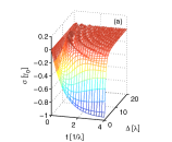
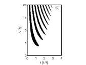
Figure 1: (Color online) (a) The rate of change $\sigma$ of the trace distance as a function of time $t$ and detuning $\Delta$ for the initial pair of states $\rho_{1}(0)=|+\rangle\langle+|$ and $\rho_{2}(0)=|-\rangle\langle-|$. (b) The black regions represent the regions in which $\sigma$ is positive.

By construction, we have ${\mathcal{N}}(\Phi)=0$ for all processes which have the divisibility property (9). In the following we discuss two simple examples for which our measure of non-Markovianity is greater than zero. The aim is to illustrate how to determine this quantity in specific cases and how non-Markovianity is related to a violation of the divisibility property and to the emergence of negative rates in master equations of the structure (6).

The first example describes a two-level system with excited state $|+\rangle$ and ground state $|-\rangle$ which interacts with a reservoir of field modes. The exact interaction picture master equation BREUER2007 describing the dynamics of the density matrix is of form of Eq. (6) with the generator (Measure for the degree of non-Markovian behavior of quantum processes in open systems), where $H(t)=0$ and we have only a single time-independent Lindblad operator $A=\sigma_{-}$ and a time-dependent rate $\gamma(t)$. The function $\gamma(t)$ is determined by the spectral density $J(\omega)$ of the reservoir. We investigate the case of a Lorentzian spectral density $J(\omega)=\gamma_{0}\lambda^{2}/2\pi[(\omega_{0}-\Delta-\omega)^{2}+\lambda^{2}]$, the center of which is detuned from the transition frequency $\omega_{0}$ of the two-level system by an amount $\Delta$, and work in the weak coupling limit $\gamma_{0}/\lambda=0.01$ (damped Jaynes-Cummings model). For sufficiently large detunings $\Delta$, the function $\gamma(t)$ then describes an exponentially damped oscillation and takes on negative values within certain intervals of time corresponding to a revival of the coherence in the system BREUER2007 ; Piilo2007 . We emphasize that this does not imply a violation of the complete positivity of the corresponding dynamical map $\Phi(t)$ because the necessary and sufficient condition for the complete positivity of $\Phi(t)$ is given by $\Gamma(t)\equiv\int_{0}^{t}dt^{\prime}\gamma(t^{\prime})\geq 0$, which is indeed satisfied here.

However, the trace distance increases for those $t$ for which $\gamma(t)<0$, i.e., we have $\sigma(t,\rho_{1,2}(0))>0$ for these times. This point is illustrated in Fig. 1 which shows $\sigma$ as a function of time $t$ and detuning $\Delta$ for the pure initial states $\rho_{1}(0)=|+\rangle\langle+|$ and $\rho_{2}(0)=|-\rangle\langle-|$. For these initial states one finds the simple expression

$$\sigma(t,\rho_{1,2}(0))=-\gamma(t)\exp[-\Gamma(t)],$$ (13)

which shows that a positive $\sigma$ and an increase of the trace distance is linked to a negative rate in the master equation. Thus, the appearance of negative rates signifies a violation of the divisibility property (9) and a flow of information from the environment back to the system.

The maximization over the pair of initial states $\rho_{1,2}(0)$ in expression (11) can be performed by drawing a sufficiently large sample of random pairs of initial states. The results are shown in Fig. 2 and provide strong numerical evidence that the maximum is attained for the initial states $\rho_{1}(0)=|+\rangle\langle+|$ and $\rho_{2}(0)=|-\rangle\langle-|$. This result could have been expected since $\rho_{2}(0)$ represents the invariant state and $\rho_{1}(0)$ has the largest distance to this state. According to Fig. 2 ${\mathcal{N}}(\Phi)$ exhibits a non-monotonic behavior: The increase of the number of intervals in which $\sigma>0$ is overcompensated for large $\Delta$ by the decrease of the size of $\sigma$ in these intervals.

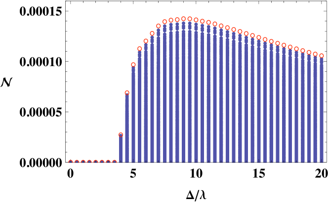
Figure 2: (Color online) The non-Markovianity ${\mathcal{N}}(\Phi)$ for the damped Janes-Cummings model as a function of the detuning $\Delta$. Blue dots: 1000 randomly drawn pairs of pure and mixed initial states. Red circles: The initial pair $\rho_{1}(0)=|+\rangle\langle+|$ and $\rho_{2}(0)=|-\rangle\langle-|$ which leads to the maximum in Eq. (11).

For the previous example the non-Markovianity ${\mathcal{N}}(\Phi)$ was found to take on finite, positive values. Our second example represents a rather extreme case, demonstrating that there are also processes for which ${\mathcal{N}}(\Phi)$ is infinite. We consider a central spin with Pauli operator $\bm{\sigma}$ which interacts with a bath of $N$ spins with Pauli operators $\bm{\sigma}^{(k)}$ through the Hamiltonian $H=A\sum_{k=1}^{N}\sigma_{z}\sigma_{z}^{(k)}$, where $A$ is a coupling constant. This simple model can easily be solved exactly BREUER2004b . Assuming the initial state of the bath to be a maximally mixed state, one finds that the populations of the density matrix of the central spin stay constant in time, while the coherences are multiplied by the factor $f(t)=\cos^{N}(2At)$. This leads to a simple formula for the trace distance of the states $\rho_{1}(t)$ and $\rho_{2}(t)$,

$$D(\rho_{1}(t),\rho_{2}(t))=\sqrt{a^{2}+f^{2}(t)|b|^{2}},$$ (14)

where $a=\rho^{++}_{1}(0)-\rho^{++}_{2}(0)$ denotes the difference of the populations, and $b=\rho^{+-}_{1}(0)-\rho^{+-}_{2}(0)$ the difference of the coherences of the two initial states. It follows that the trace distance oscillates periodically between $D_{\max}=\sqrt{a^{2}+|b|^{2}}$ and $D_{\min}=|a|$. This can be interpreted as a periodic oscillation of the distinguishability of the two states, i.e., as a periodic exchange of information between the central spin and the spin bath.

The maximal growth of the trace distance occurs if one takes as initial states the two eigenstates of $\sigma_{x}$, or any other pair of states corresponding to antipodal points on the equator of the Bloch sphere, such that $a=0$ and $|b|=1$. The trace distance then oscillates periodically between the values $1$ and $0$. The sum in Eq. (12) therefore diverges and we obtain ${\mathcal{N}}(\Phi)=+\infty$, which implies that a Markovian approximation of the system dynamics is never possible. One can formally write a master equation of the form (6) with $H=0$, a single Lindblad operator $A=\sigma_{z}$ and the rate $\gamma(t)=AN\tan(2At)$, which shows again the connection between the growth of the trace distance and the emergence of negative rates.

Summarizing, we have constructed a measure ${\mathcal{N}}(\Phi)$ for the non-Markovianity of quantum processes in open systems. The definition (11) of the measure neither relies on any specific representation or approximation of the dynamics, nor does it presuppose the existence of a master equation or of invariant states. The exact determination of the measure generally requires solving the complete reduced system dynamics which could be a difficult task for more complex problems. However, any observed growth of the trace distance is a clear signature for non-Markovian behavior and leads to a lower bound for ${\mathcal{N}}(\Phi)$. The measure for non-Markovianity introduced here could therefore be useful also for the experimental validation of theoretical models or approximation schemes. To detect non-Markovianity experimentally one has to perform a state tomography on different ensembles at different times in order to decide whether or not the trace distance has increased. A great advantage of the present approach is given by the fact that it allows to plan experiments which test non-Markovianianity without knowing anything about the properties of the environment or about the structure of the system-environment interaction. Hence, we think that our measure is a useful tool for the characterization of non-Markovianity, both in theoretical descriptions and in experiments.

- (1) V. Gorini, A. Kossakowski, and E. C. G. Sudarshan, J. Math. Phys. 17, 821 (1976).
- (2) G. Lindblad, Commun. Math. Phys. 48, 119 (1976).
- (3) H. P. Breuer and F. Petruccione, The Theory of Open Quantum Systems (Oxford University Press, Oxford, 2007).
- (4) J. Piilo, S. Maniscalco, K. Härkonen and K.-A. Suominen, Phys. Rev. Lett. 100, 180402 (2008); J. Piilo, K. Härkonen, S. Maniscalco and K.-A. Suominen, Phys. Rev. A 79, 062112 (2009); H. P. Breuer and J. Piilo, EPL 85, 50004 (2009).
- (5) M. M. Wolf, J. Eisert, T. S. Cubitt, and J. I. Cirac, Phys. Rev. Lett. 101, 150402 (2008).
- (6) H. P. Breuer and B. Vacchini, Phys. Rev. Lett. 101, 140402 (2008); Phys. Rev. E 79, 041147 (2009).
- (7) H. P. Breuer, Phys. Rev. A 70, 012106 (2004).
- (8) D. Chruściński, A. Kossakowski and S. Pascazio, eprint arXiv:0906.5122v1 [quant-ph].
- (9) H. Krovi, O. Oreshkov, M. Ryazanov, and D. A. Lidar, Phys. Rev. A 76, 052117 (2007).
- (10) A. J. van Wonderen and K. Lendi, Europhys. Lett. 71, 737 (2005); J. Phys. A 39, 14511 (2006).
- (11) A. A. Budini, Phys. Rev. A 74, 053815 (2006).
- (12) S. M. Barnett and S. Stenholm, Phys. Rev. A 64, 033808 (2001).
- (13) J. Wilkie and Y. M. Wong, J. Phys. A 42, 015006 (2009).
- (14) S. Daffer, K. Wodkiewicz, J. D. Cresser, and J. K. McIver, Phys. Rev. A 70, 010304(R) (2004).
- (15) A. Kossakowski and R. Rebolledo, Open Syst. Inf. Dyn. 15, 135 (2008); Open Syst. Inf. Dyn., to be published.
- (16) M. M. Wolf and J. I. Cirac, Commun. Math. Phys. 279, 147 (2008).
- (17) M.A. Nielsen and I. L. Chuang, Quantum Computation and Quantum Information (Cambridge University Press, Cambridge, 2000).
- (18) M. B. Ruskai, Rev. Math. Phys. 6, 1147 (1994).
- (19) H. P. Breuer, Eur. Phys. J. D 29, 105 (2004).