A method to measure a relative transverse velocity of source-lens-observer system using gravitational lensing of gravitational waves

Abstract

Gravitational waves propagate along null geodesics like light rays in the geometrical optics approximation, and they may have a chance to suffer from gravitational lensing by intervening objects, as is the case for electromagnetic waves. Long wavelength of gravitational waves and compactness of possible sources may enable us to extract information in the interference among the lensed images. We point out that the interference term contains information of relative transverse velocity of the source-lens-observer system, which may be obtained by possible future space-borne gravitational wave detectors such as BBO/DECIGO.

I Introduction

Direct observations of gravitational waves from astrophysical sources would open a new window to the universe, and a new era of astronomy. It is now well known that there are many gravitational lens systems of various sorts in the electromagnetic astronomy. This must also happens in gravitational wave astronomy in the future. One difference between electromagnetic waves and gravitational waves are their wavelength. The wavelength of gravitational waves which the currently working and the planned gravitational wave observatories may detect are typically much larger than the electromagnetic waves in the current astronomy. Therefore once they suffer from gravitational lensing, we have a chance to observe interference. To be more quantitatively, a condition may be met for interference to be seen. In the electromagnetic astronomy, a wave source is typically extended and it consists of pieces of incoherent emitters. Then, to observe interference, the typical linear dimension of the source $l$ should be smaller than or comparable to the wavelength $\lambda$ divided by the angular separation among the multiple images $\theta$ (in radians), or $l\lower 2.15277pt\hbox{$\;\buildrel<\over{\sim}\;$}\kappa\lambda/\theta\equiv\kappa l_{0}$ with $\kappa$ of order unity in a typical gravitational lensing occurring in cosmology. Otherwise incoherent waves from different parts of the source distract the interference. Observing at, say, $\lambda=1\mu$m and assuming $\theta=10^{\prime\prime}\simeq 5\times 10^{-5}$ radians, $l_{0}\simeq 2$ cm. This is one reason why we usually do not see interference in the electromagnetic astronomy. One exception where wave effects become important is scintillation for radio sources due to ionized interstellar/interplanetary gas (See, e.g., Chap. 13.4 of Thompson et al. (2001)). As an application, for example, the size of a gamma-ray burst (GRB) can be estimated using the interstellar scintillation of radio afterglow of a GRB (See, e.g., Frail et al. (1997)). On the other hand, there are compact gravitational wave sources whose linear sizes are of order the wavelength they emit. These include relativistic coalescing binaries such as neutron stars binaries and isolated non-axisymmetric pulsars, both of which are two of the most promising sources (e.g., Cutler and Thorne (2002)) for the gravitational wave detectors that are currently working or planned, such as LIGO Abramovici et al. (1992), LCGT Kuroda et al. (1999), LISA Danzmann and et al. (1996), BBO Phinney and et al. (2003), and DECIGO Seto et al. (2001). At around the BBO/DECIGO observing frequency of $f=0.1$Hz, the orbital separation $l$ of a neutron stars binary would be $l\sim 10^{4}{\rm km}(2M_{\rm NS}/2.8M_{\odot})^{1/3}(f/0.1{\rm Hz})^{-2/3}$, while $l_{0}\sim 4\times 10^{2}{\rm AU}(f/0.1{\rm Hz})^{-1}(\theta/10^{\prime\prime})^{-1}>>$ $l$.

In the above argument, we saw that there is an upper limit on the size of the emitter to see interference. This is not a sufficient condition for interference pattern to form in the space and for us to observe its amplitude changing as the Earth (or a detector) moves in that spatial pattern. For a clear interference pattern to form in the space, coherence time must be larger than the time delay among multiple images. Note that the coherence time is of order $1/\Delta f$ where $\Delta f$ is the frequency shift during an observation. Suppose an extragalactic neutron stars binary as a gravitational wave source. Then to have a large enough signal to noise ratio with BBO/DECIGO to claim detection, we may integrate the signal from the binary for a couple of years during which the signal frequency of the source binary would shift over of order of the BBO/DECIGO observing frequency, $f\sim\Delta f\sim 0.1$ Hz. The coherence time would then be $10$ seconds, which is smaller than, for example, the time delays of the known gravitational lensing systems listed in the CASTLE data base Kochanek et al. (2006); Muñoz et al. (1998). So unless the time delay is smaller than $\sim 10$ seconds or the source is highly monochromatic, we are not in a situation where we (on the Earth) move in a clear spatial interference pattern.

The above argument does not preclude a possibility of detecting an interference term in the time domain, or equivalently, in the frequency domain. In this paper, we do not aim to detect an interference pattern in the space. Rather, we propose a method of a filtered cross-correlation of gravitational lens images in the frequency domain. We shall point out that the interference term contains information of the relative transverse velocity of the source-lens-observer system and study how well we could determine it using the future BBO/DECIGO detector.

There have already been several works that point out importance of interference and, more broadly, wave optics effects in gravitational lensing phenomena of gravitational waves Peterson and Falk (1991); Takahashi (2004); Matsunaga and Yamamoto (2006); Takahashi (2006); Yoo et al. (2007). Since a gravitational wave source such as a coalescing binary is essentially a point source, we have to use wave optics rather than geometrical optics approximation for such a source near caustics Schneider et al. (1992); Baraldo et al. (1999). The works Takahashi (2006); Yoo et al. (2007) studied observable effects on the gravitational waves propagating in an inhomogeneous universe. In this paper, we propose a method for extracting an interference term in the geometrical optics limit and for obtaining information on a relative transverse velocity of the source-lens-observer system. There are various methods to measure a relative transverse velocity of astronomical objects at a cosmological distance in the electromagnetic astronomy. Those includes for example, a method to measure transverse velocities of clusters of galaxies detecting a signature of gravitational scattering of the cosmic microwave background Birkinshaw and Gull (1983); Pyne and Birkinshaw (1993); Aso et al. (2002) and to measure those of galaxies using a parallax effect due to gravitational micro-lensing Grieger et al. (1986); Gould (1995). Possibilities are also discussed in in the gravitational lens literature by Molnar and Birkinshaw (2003). Gravitational lensing of gravitational waves possibly offers another way to measure a relative transverse velocity of cosmological objects in addition to those methods above.

Our method could be applied to various sources including continuous waves from pulsars, cosmic strings and so on. However, to be specific, we consider a coalescence neutron stars binary at a cosmological distance.

This paper is organized as follows. In the next section, we explain our situation by discussing a (astronomical scale) Young’s interference experiment. In Sec. III, we remind readers of the basic equations and the notations for study of gravitational lensing of gravitational waves, for which we follow Takahashi and Nakamura (2003). After remarks on a situation we would be in when searching for gravitational lensing of gravitational waves and on the geometrical optics approximation, Sec IV explains how to extract interference term when the approximation applies. In the section V, we propose a method for extracting information contained in the interference term, namely, the relative transverse velocity of the source-lens-observer system. We then study a correlation between the time delay and the transverse velocity in Sec VI and a correlation among parameters in VII in the absence of noise. Sec. VIII then shows the precision to which we could measure a transverse velocity by introducing detector noise. The section IX gives summary of our result.

In this paper we use a unit of $G=c=1$ unless otherwise written explicitly. An amplitude of a gravitational wave inversely depends on the luminosity distance from the observer to the source, to compute which we assume a flat universe with $\Omega_{\Lambda}=0.7$, $\Omega_{{\rm matter}}=0.3$, and $h=0.7$.

II Young’s interference experiment

To explain our situation, consider the (astronomical scale) Young’s two pin-holes interference experiment. The (gravitational) wave intensity $I$ at the observer’s time and position $(t,x)$ on the screen is

$$I(t,x) = \left|\frac{1}{r_{1}}e^{i\sigma_{1}}+\frac{1}{r_{2}}e^{i\sigma_{2}}\right|^{2}\simeq 2\frac{1}{r^{2}}(1+\cos(\sigma_{1}-\sigma_{2})),$$ (1)

where $r_{k}$ is the distance from the $k$-th pin-hole to the observer and $\sigma_{k}$ is the phase of the wave from the $k$-th pin-hole. We neglect the difference in $r_{1}$ and $r_{2}$ in the amplitude and write $r_{1}\simeq r_{2}\equiv r$. The phase difference $\sigma(t,x)\equiv\sigma_{1}-\sigma_{2}$ may be written as

$$\sigma(t,x)=2\pi\int_{t_{r}}^{t_{r}+\Delta t_{d}(t,x)}f(t^{\prime})dt^{\prime},$$ (2)

where $t_{r}=t_{r}(t,x)=t-\tau_{1}(t,x)$ is the source retarded time for the wave through the pin-hole 1, $\tau_{k}(t,x)$ is the time length for a wave crest to propagate from the source to the observer through the $k$-th pin-hole, and $\Delta t_{d}(t,x)=\tau_{2}(t,x)-\tau_{1}(t,x)$ is the time delay between two pin-holes.

For a monochromatic wave at the frequency $f(t)=f_{c}=$ constant, $\sigma(t,x)=2\pi f_{c}\Delta t_{d}(t,x)$ and the scale of the interference pattern is $\Delta x=c/\theta/f/2$ ($\theta$ being the angular separation of the two pin-holes seen from the observer) as usual. Known possible monochromatic gravitational wave sources are isolated pulsars. The planned next generation gravitational wave antennas would see those within the Milky way galaxy. So considering micro-lensing phenomena on a gravitational wave emitted by an isolated millisecond pulsar in a globular cluster (say), the spatial scale of the interference pattern is

$$\Delta x \simeq 3\times 10^{10}{\rm km}\left(\frac{1{\rm mas}}{\theta}\right)\left(\frac{1{\rm kHz}}{f_{c}}\right)\simeq 200{\rm AU}.$$ (3)

Suppose, in the spatial interference pattern due to the monochromatic wave, we move at 200 km/s (about the orbital speed of the Solar system around the Galactic center), it takes $\sim 5$ years for us to go across the spatial interference pattern. The wave intensity will vary in time as

$$I(t,x)\sim\cos\left(2\pi\frac{fv\theta}{c}t+{\rm const}.\right)+{\rm const}.$$ (4)

In principle, for a monochromatic wave, we would be able to detect relative transverse velocity of the source-lens-observer system by using interference pattern (by measuring the temporal variation of $I(t,x)$). If we recognise such interference pattern, we would conclude that gravitational force shows interference phenomena and propagate as “wave”. Other than that, the information we could obtain, $v\theta$, is in principle the same as that in micro-lensing experiments in the conventional electromagnetic astronomy. (And the number of millisecond pulsars is much smaller than that of the stars in the Magellanic clouds, say.)

When observing pulsars within the Milky way, it is also important to note that diffraction effect becomes non-negligible when gravitational wavelength $\lambda$ is larger than the lens mass $M_{L}$ Takahashi and Nakamura (2003), or $M_{L}\lower 2.15277pt\hbox{$\;\buildrel<\over{\sim}\;$}10^{2}M_{\odot}(f/1{\rm kHz})^{-1}$. If we observe interference of gravitational waves from pulsars in the Milky way, then the lens should have mass larger than $\sim 10^{2}M_{\odot}$

Eq. (3) suggests a cosmological application of gravitational lensing phenomena on gravitational waves.

$$\frac{\Delta x}{v} \simeq 5{\rm years}\left(\frac{200{\rm km/s}}{v}\right)\left(\frac{10^{\prime\prime}}{\theta}\right)\left(\frac{0.1{\rm Hz}}{f_{c}}\right).$$ (5)

Unfortunately for our purpose of seeing an interference pattern, the most promising cosmological sources, relativistic compact binaries in an inspiralling phase, do not emit monochromatic wave. For such a source the frequency of the gravitational wave varies in time, to the lowest order,

$$\frac{df}{dt} = \frac{96\pi^{8/3}}{5}\left(\frac{GM_{\rm c}}{c^{3}}\right)^{5/3}f^{11/3},$$ (6)

with $M_{\rm c}=(m_{1}m_{2})^{5/3}/(m_{1}+m_{2})^{1/5}$ is the chirp mass, $m_{k}$ being the mass of the $k$-th star in the binary. For wave having time-varying frequency $df(t)/dt=Af^{\eta}(t)$ with $A$ and $\eta$ constants,

$$\frac{\sigma(t,x)}{2\pi} = ((\eta-1)(t_{c}-t-\Delta t_{d}(t,x))A+f_{{\rm max}}^{1-\eta})^{\frac{1}{1-\eta}}-((\eta-1)(t_{c}-t)A+f_{{\rm max}}^{1-\eta})^{\frac{1}{1-\eta}},$$ (7)

with $f(t=t_{c})=f_{{\rm max}}$ at which inspiralling phase ends and the binary stars crush into each other. The interference pattern changes with time even if there is no relative transverse velocity in the system. Moreover because of the smallness of the amplitudes of possible gravitational waves, we normally need to integrate signals for some time duration to get a sufficiently-large-for-claiming-detection signal to noise ratio. Schematically, we would do

$$\int^{T_{{\rm obs}}}_{0}I(t^{\prime},vt^{\prime}+{\rm const}.)dt^{\prime}.$$ (8)

$T_{{\rm obs}}$ is determined by either the source lifetime, its pass-time over the frequency band of our detector, or a pre-set threshold for claiming detection (, say, signal to noise ratio larger than 5). Large $T_{{\rm obs}}$ in the integration makes the interference term vanishingly smaller than the bolometric (non-interference) term. For a massive compact binary, depending on binary masses, it is possible that $T_{{\rm obs}}<<({\rm time}\,\,{\rm delay})$ so that one wave packet through the pin-hole 1 comes to the detector, and after some quiet period, the second through the pin-hole 2 visits it. In this case, no interference pattern forms in the space and we would detect their interference by taking a cross-correlation (in a computer). This paper shall use a filtered cross-correlation technique to take care of the issues above. But before moving onto explaining the technique we use in this paper, we start our discussion by explaining lensed waveform of gravitational waves in the next section.

III Lensed waveform of gravitational wave

We consider a coalescence compact stars binary at the redshift $z_{S}$ with the redshifted chirp mass ${M}_{cz}={M}_{c}(1+z_{S})$ as a target source to be lensed. The detector is assumed to be a space borne interferometer such as (one-triangle) BBO/DECIGO, which outputs two independent data streams $h_{\alpha=I,II}(f)$. When the gravitational wave from the binary is lensed by a lensing object of redshifted mass $M_{Lz}=M_{L}(1+z_{L})$, the wave through the $j$-th image to the detector in the frequency domain would be written, in the geometrical optics limit and in the stationary phase approximation, as Takahashi and Nakamura (2003)

$$h_{\alpha,j}^{L}(f) = \frac{\sqrt{3}}{2}|\mu_{j}|^{1/2}\Lambda_{\alpha,j}(t_{j})e^{-i\pi n_{j}-i\Phi_{\alpha,j}(t_{j})}Af^{-7/6}e^{i\Psi_{j}(f)},$$ (9)

with

$$\Phi_{\alpha,j}(t) = \phi_{D,j}(t)+\phi_{p,j,\alpha}(t),$$ (10)

where $n_{j}=0,1/2$ and 1 when the j-th image corresponds to a minimum, saddle, and maximum point, respectively. $\Lambda_{\alpha,j}(t)$ is written in terms of the detector beam pattern functions $F_{\alpha}^{+}(t),F_{\alpha}^{\times}(t)$ Cutler (1998) and defined as

$$\Lambda_{\alpha,j}(t) = \left((1+(\vec{L}\cdot\vec{N}_{j})^{2})^{2}F_{\alpha}^{+}(t)+4(\vec{L}\cdot\vec{N}_{j})^{2}F_{\alpha}^{\times}(t)\right)^{1/2},$$ (11)

where $\vec{L}$ (given by $\bar{\theta}_{L},\bar{\phi}_{L}$) and $\vec{N}_{j}$ (given by $\bar{\theta}_{S,j},\bar{\phi}_{S,j}$) are the direction unit vector of the binary orbital angular momentum and the direction unit vector toward the j-th image. These vectors are defined in the fixed barycenter frame of the solar system. The detector phase $\phi_{D,j}(t)$ and the source phase $\phi_{p,j,\alpha}(t)$ are

$$\phi_{D,j}(t) = 2\pi f(t)R\sin\bar{\theta}_{S,j}\cos\left(\bar{\phi}(t)-\bar{\phi}_{S,j}\right),$$ (12)

$$\phi_{p,j,\alpha}(t) = \tan^{-1}\left(\frac{2(\vec{L}\cdot\vec{N}_{j})F^{\times}_{\alpha}(t)}{(1+(\vec{L}\cdot\vec{N}_{j})^{2})F^{+}_{\alpha}(t)}\right),$$ (13)

where $\bar{\phi}(t)=2\pi t/T+\bar{\phi}_{0}$ with $R=1{\rm AU}$ and $T=$ 1 year for BBO/DECIGO (Those detectors are planned to orbit around the solar system barycenter with its average orbital radius 1 AU. For simplicity we assumed a circular orbit for the detector here). The amplitude of the gravitational wave $A$ and the phase of the gravitational wave $\Psi_{j}(f)$, to the Newtonian approximation, are

$$\Psi_{j}(f) = 2\pi ft_{d,j}+\Psi(f)=2\pi ft_{c,j}-\phi_{c}-\frac{\pi}{4}+\frac{3}{4}\left(8\pi{M}_{cz}f\right)^{-5/3},$$ (14)

$$A = \frac{1}{D_{S}(1+z_{S})^{2}}\left(\frac{5}{96}\right)^{1/2}\pi^{-2/3}{M}_{cz}^{5/6},$$ (15)

where $D_{S}$ is the source angular diameter distance. $\mu_{j}$ and $t_{d,j}$ are the amplification factor and the time delay for the j-th image measured with respect to the fictitious time of arrival of non-lensed signal. $t_{c,j}=t_{c}+t_{d,j}$. $t_{c}$ and $\phi_{c}$ are the time and the phase of the binary coalescence. Finally, the time variable $t$ in the above equations must be understood to be a function of frequency as

$$t(f) = =t_{c}-5(8\pi f)^{-8/3}{M}_{cz}^{-5/3},$$ (16)

$$t_{j}(f) = t(f)+t_{d,j}=t_{c,j}-5(8\pi f)^{-8/3}{M}_{cz}^{-5/3}.$$ (17)

In a gravitational wave search, the unknown parameters would be, to the lowest order,

$$\{{M}_{cz},\phi_{c},t_{c},D_{S},\bar{\theta}_{S,j},\bar{\phi}_{S,j},\vec{L},\kappa_{1}-\kappa_{2},\Delta t_{d}=t_{d,2}-t_{d,1},|\mu_{1}|/|\mu_{2}|\},$$ (18)

where the last three depend on the lens property.

IV Search for a lensed gravitational wave

We consider the following situation. First of all, for simplicity we study that two images occur due to gravitational lensing. Then the wave from one lens image would be in the detector’s observation frequency band in the time duration from, say, $t_{s,1}$ to $t_{e,1}$. The second wave would be in the band after the time delay $\Delta t_{d}$ later from $t_{s,2}=t_{s,1}+\Delta t_{d}$ to $t_{e,2}=t_{e,1}+\Delta t_{d}$. We assume the observation frequency and the time delay satisfy $f\Delta t_{d}\sim 0.1(f/0.1{\rm Hz})\Delta t_{d}>>1$ so that we can use the geometrical optics approximation (Takahashi and Nakamura (2003) studied the case where wave optics is important). As as result, we may detect the two waves separately using unlensed waveform templates as if those were unlensed, in the same sky direction (The angular resolution of the gravitational wave source is $\sim 10^{-2}$(Signal to noise ratio)^-1 radians with the current BBO design Cutler and Harms (2006), so we do not expect to resolve images). We would then realize that those two waves have similar parameters sets ${M}_{cz},\phi_{c},\vec{L}$, and conclude that those two are actually due to one lensed event. We may find the (relative) time delay $\Delta t_{d}=t_{d,2}-t_{d,1}$ and the ratio of the magnification $|\mu_{1}|^{1/2}/|\mu_{2}|^{1/2}=A_{1}/A_{2}$. The observational errors of these two numbers are at the same level as those of $t_{c}$ and $A$. We might now cross-correlate the two waves to see interference between these two (in a computer). However, a simple cross-correlation disappears when the geometrical optics approximation applies (and this is the reason we could detect two waves separately, anyway). Let us see this using some equations below and propose a method to extract information contained in the interference term even in this case.

IV.1 How to extract the interference term when the geometrical optics approximation applies

We consider a sort of cross-correlation between the two waves, given by (9). We use the waves with the supports in the time domain assumed to be from $t_{e,1}-\Delta t_{d}$ to $t_{e,1}$ for the wave that reaches the detector first, and from $t_{e,2}-\Delta t_{d}=t_{e,1}$ to $t_{e,2}$ for the second. The detector’s output $s_{k}(t)$ in the two time segments ($k=A,B$) are

$$s_{A}(t) = \sum_{j}h_{j}(t)\,\,\,{\rm for}\,\,\,t_{e,1}-\Delta t_{d}\leq t\leq t_{e,1},$$ (19)

$$s_{B}(t) = h_{2}(t)\,\,\,{\rm for}\,\,\,t_{e,1}\leq t\leq t_{e,2}.$$ (20)

The Fourier expansions of the gravitational wave $h_{1}(t)$ in the time segment $A$ and that of $h_{2}(t)$ in the time segment $B$ have a support from $f_{i}$ to $f_{e}$ in the frequency domain. The frequency domain support of $h_{2}(t)$ in the time segment $A$ is lower than $f_{i}$ . We now compute a simple cross-correlation between the two waves as

$$4Re\int_{f_{i}}^{f_{e}}\frac{s_{A}(f)s_{B}^{*}(f)}{S_{h}(f)}df = 4Re\sum_{\alpha}\int_{f_{i}}^{f_{e}}\frac{h_{\alpha,1}^{L}(f)h_{\alpha,2}^{L*}(f)}{S_{h}(f)}df,$$ (21)

with $S_{h}$ the one-sided spectral density of the detector’s noise. Because we defined the integral region from $f_{i}$ to $f_{e}$ so that there is no auto-correlation term of $h_{\alpha,2}^{L}(f)$ which otherwise appears due to $h_{2}(t)$ term in $s_{A}(t)$. Now, $h_{\alpha,j}^{L}(f)$ is given by Eq. (9) and the simple cross-correlation becomes

$$4Re\int_{f_{i}}^{f_{e}}\frac{h_{\alpha,1}^{L}(f)h_{\alpha,2}^{L*}(f)}{S_{h}(f)}df$$ (22)

$$= \frac{3}{2}|\mu_{1}|^{1/2}|\mu_{2}|^{1/2}A^{2}$$

$$\times Re\int_{f_{i}}^{f_{e}}\frac{f^{-7/3}}{S_{h}(f)}\Lambda_{\alpha,1}(t_{1})\Lambda_{\alpha}(t_{2})e^{2\pi if\Delta t_{d}-i\pi(\kappa_{1}-\kappa_{2})}e^{i\Phi_{\alpha,2}(t_{2})-i\Phi_{\alpha,1}(t_{1})}df.$$

This integrand is oscillatory and the result is effectively zero if $|f\Delta t_{d}|>>1$.

Now, how can we extract non-zero cross-correlation? We propose a filtered cross-correlation statistic. We multiply the two images, and before the frequency domain integration we further multiply $\cos(2\pi f\Delta t^{T}_{d}+\Theta(f,{\mathbf{p}^{T}}))$ where $\Delta t_{d}=t_{d,2}-t_{d,1}$, the tuplet $\mathbf{p}=(t_{c,1},t_{c,2},M_{cz},\kappa_{1}-\kappa_{2},\vec{N},\vec{L})$,

$$\Theta(f,\mathbf{p})\equiv\Phi_{\alpha,2}(t_{2}(f))-\Phi_{\alpha,1}(t_{1}(f))+\pi(\kappa_{1}-\kappa_{2}),$$ (23)

and $\mbox{}^{T}$ denoting a template. We define our detection statistic $\zeta_{\alpha}$ as

$$\zeta_{\alpha} = 4Re\int_{f_{i}}^{f_{e}}\frac{h^{L}_{\alpha,1}(f)h^{L*}_{\alpha,2}(f)}{S_{h}(f)}\cos(2\pi f\Delta t^{T}_{d}+\Theta(f,{\bf p}^{T}))df$$ (24)

$$\simeq 3|\mu_{1}|^{1/2}|\mu_{2}|^{1/2}A^{2}$$

$$\times \int_{f_{i}}^{f_{e}}\frac{f^{-7/3}}{S_{h}(f)}\Lambda_{\alpha,1}(t_{1})\Lambda_{\alpha,2}(t_{2})\cos(2\pi f(\Delta t_{d}-\Delta t_{d}^{T})+\Theta(f,\mathbf{p})-\Theta(f,{\mathbf{p}^{T}}))df.$$

Maximizing an absolute value of the detection statistic $|\zeta|$ (where $\zeta\equiv\sum_{\alpha}\zeta_{\alpha}$), we obtain our estimate of the time delay $\Delta t_{d}$. In the next section we study an effect on our statistic $\zeta$ of a relative transverse velocity of the source-lens-observer system. In the later sections, we shall study precision to which we could measure $\Delta t_{d}$ and the transverse velocity and correlations among errors of the parameters $\Delta t_{d}$, the transverse velocity, and ${\bf p}$.

V Transverse velocity

We can measure $\{t_{c,j},{M}_{cz},\bar{\theta}_{S},\bar{\phi}_{S},\vec{L},n_{j}\}$ using gravitational lensing phenomena in the usual electromagnetic astronomy. When one can use information in an interference term, we could get new information on the lens/source object: its relative transverse velocity. When there is a relative velocity among the source-lens-observer, there may be two effects. One is the time variation of the direction of the images $\vec{N}_{j}$, which may not be detected for cosmological sources in the foreseeable future because of the poor pointing ability of the planned gravitational wave detectors. The other is the Doppler effect which causes rescaling of the mass of the source, the time variables and the amplitudes of the gravitational waves. The rescaling due to the Doppler effect differs for different images as

$$\tilde{t}_{jk}(f) = \tilde{t}_{c,jk}-5(8\pi f)^{-8/3}\tilde{M}_{cz,k}^{-5/3},$$ (25)

and $\tilde{M}_{cz,j}=\gamma_{j}{M}_{cz},\tilde{t}_{c,jk}=\gamma_{k}t_{c,j},$ and $\tilde{A}_{j}=\gamma_{j}^{-7/6}A$ with $\gamma_{j}=(1+\vec{N}_{j}\cdot\vec{\beta}),$ where the velocity $\vec{\beta}=\vec{v}/c$ is a linear combination of the observer velocity $\vec{v}_{O}$, the lens velocity $\vec{v}_{L}$, and the source velocity $\vec{v}_{S}$ as Kayser et al. (1986); Wucknitz and Sperhake (2004)

$$\vec{v} = \vec{v}_{O}+\frac{1+z_{L}}{1+z_{S}}\frac{D_{L}}{D_{LS}}\vec{v}_{S}-\frac{D_{LS}+D_{L}}{D_{LS}}\vec{v}_{L},$$ (26)

with $D_{LS}$ being the angular diameter distance between the lens and the source.

The lensed gravitational waveform from a coalescing binary now becomes

$$\tilde{h}_{\alpha,j}^{L}(f) = \frac{\sqrt{3}}{2}|\mu_{j}|^{1/2}\Lambda_{\alpha,j}(\tilde{t}_{jj})e^{-i\pi n_{j}}e^{-i\Phi_{\alpha,j}(\tilde{t}_{jj})}\tilde{A}_{j}f^{-7/6}e^{i\tilde{\Psi}_{jj}(f)},$$ (27)

with

$$\tilde{\Psi}_{jk}(f) = 2\pi f\tilde{t}_{c,jk}-\phi_{c}-\frac{\pi}{4}+\frac{3}{4}\left(8\pi\tilde{M}_{cz,k}f\right)^{-5/3}.$$ (28)

If there is only one image, then we could not resolve the degeneracy and would get, in principle, a biased estimate of the masses and the source distance. However, if we know in advance that we see multi-waves due to gravitational lensing (see Sec. IV), then we could find the differences of the Doppler factors among different images.

For later convenience, we introduce a notation for the ratio of the Doppler factors as

$$\Gamma = \frac{\gamma_{1}}{\gamma_{2}}=1+(\vec{N}_{1}-\vec{N}_{2})\cdot\vec{\beta}+O(\beta^{2}).$$ (29)

Note that $\Gamma-1\simeq\theta\beta_{\perp}$ where $\theta$ is the angular size of the lens. Finding $\Gamma$ using the interference term of the lensed gravitational wave then gives us the transverse velocity $\beta_{\perp}$ , given that $\theta$ is known from, say, electromagnetic observation of the lens object (say, galaxies/clusters) and the host object (say, a galaxy) of the gravitational wave source.

We compute a cross-correlation between the lensed wave with itself but with frequency shifted by $\Gamma^{T}$ here $\mbox{}^{T}$ denoting a template, and further multiply the cosine filter as in the previous section,

$$\zeta_{\alpha} = 4Re\int_{f_{i}}^{f_{e}}\frac{df}{S_{h}(f)}\tilde{h}^{L}_{\alpha,1}(f)\tilde{h}^{L*}_{\alpha,2}\left(\Gamma^{T}f\right)\cos(2\pi f\Delta\tilde{t}^{T}_{d,1}+\Theta(f,\mathbf{p}^{T})))$$ (30)

$$\simeq 3|\mu_{1}|^{1/2}|\mu_{2}|^{1/2}\tilde{A}_{1}\tilde{A}_{2}Re\int_{f_{i}}^{f_{e}}\frac{df}{S_{h}(f)}f^{-7/3}{\cal H}\cos(2\pi f\Delta\tilde{t}^{T}_{d,1}+\Theta(f,\mathbf{p}^{T}))).$$

The function ${\cal H}$ is defined as

$${\cal H} = \Lambda_{\alpha,1}(\tilde{t}_{11}(f))\Lambda_{\alpha,2}(\tilde{t}_{22}(\Gamma^{T}f))$$ (31)

$$\times e^{i\Phi_{\alpha,2}(\tilde{t}_{22}(\Gamma^{T}f))-i\Phi_{\alpha,1}(\tilde{t}_{11}(f))}e^{i\tilde{\Psi}_{11}(f)-i\tilde{\Psi}_{22}(\Gamma^{T}f)},$$

with

$$\tilde{\Psi}_{11}(f)-\tilde{\Psi}_{22}(\Gamma^{T}f) = 2\pi f\tilde{t}_{c,11}+\frac{3}{4}\left(8\pi\tilde{M}_{cz,1}f\right)^{-5/3}$$ (32)

$$-2\pi f\Gamma^{T}\tilde{t}_{c,22}-\frac{3}{4}\left(8\pi\Gamma^{T}\tilde{M}_{cz,2}f\right)^{-5/3}.$$

The parameters to be searched for are, in addition to the parameters $\mathbf{p}^{T}$, the time delay between images, $\Delta t_{d}$, and the $\Gamma$ parameter. When $\Gamma^{T}\simeq 1+\theta\beta_{\perp}+\delta(\theta\beta_{\perp})$ with $\theta\beta_{\perp}<<1$ and $\delta(\theta\beta_{\perp})<<1$,

$$\tilde{\Psi}_{11}(f)-\tilde{\Psi}_{22}(\Gamma^{T}f) \simeq 2\pi f\Delta\tilde{t}_{d,1}-2\pi f\tilde{t}_{22}(f)\delta(\theta\beta_{\perp}),$$ (33)

with $\Delta\tilde{t}_{d,1}=\gamma_{1}\Delta t_{d}$.

Eq. (33) tells us that larger the observation frequency $f$ is, and/or longer the observation time is, with a better precision we measure the time delay $\Delta t_{d}$ and/or $\Gamma$ . This latter tendency will be studied further in the sections VII and VIII. Eq. (33) also indicates a correlation between $\Delta t_{d}$ and $\Gamma$, which we will study in the next section.

VI Correlation between the time delay and the transverse velocity

When one uses usual matched filtering technique to unlensed gravitational waves, the search parameters are 8 in the lowest order (See the list (18)). To find the transverse velocity of the source, in addition to those, we search for two parameters: the time delay $\Delta t_{d}$ and the transverse velocity $\Gamma$. Since these two parameters are the new aspects in our paper, in this section we show how our detection statistic $\zeta$ (where $\zeta\equiv\sum_{\alpha}\zeta_{\alpha}$) depends on these two parameters.

To demonstrate a correlation between $\Delta t_{d}$ and $\Gamma$, we consider a source with the parameters listed in the table LABEL:tbl:Q0957+561. The source redshift $z_{S}$, the lens redshift $z_{L}$, the image separation $\theta$, the time-delay and the direction of the source are taken from the famous lens system Q0957+561 Walsh et al. (1979); Kochanek et al. (2006). With those parameters, we compute our statistic $\zeta$ in the $\Gamma^{T}$-$\Delta t_{d}^{T}$ plane with other parameters fixed to be the right values. Fig. 1 shows the contour map of $\zeta$, which clearly shows a strong correlation between $\Gamma^{T}$ and $\Delta t_{d}^{T}$. As can be inferred from Eq. (33), the correlation is found well approximated by

$$\Delta t_{d}^{T}-\Delta t_{d} = -(\Gamma^{T}-\Gamma)T_{{\rm obs}},$$ (34)

near $\Delta t_{d}^{T}=\Delta t_{d}$. In fact, along this line and projected onto $\Gamma$, the detection statistic behaves as in Fig. 2, which shows the maximum appears at $\Gamma^{T}\simeq\Gamma$: The maximum of $\zeta$ occurs slightly shifted $\Gamma^{T}$ value from the true value ($\sim 1\%$). This happens because in Eq. (30), we should have used instead of $\Theta(f,{\bf p})$ defined in Eq. (23), $\tilde{\Theta}(f,{\bf p})$ of the form

$$\tilde{\Theta}(f,\mathbf{p})=\Phi_{\alpha,2}(t_{2}(\Gamma f))-\Phi_{\alpha,1}(t_{1}(f))+\pi(\kappa_{1}-\kappa_{2}).$$ (35)

Unfortunately, since use of this $\tilde{\Theta}$ demanded large computational power in our code, we used $\Theta$ instead paying $\sim 1\%$ bias in $\Gamma-1$.

Table 1: The source, lens, detector parameters for the figures 1 and 2. Here $T_{{\rm obs}}$ is the integration time (time for the wave to pass the frequency band from $f_{i}$ Hz to $f_{e}$ Hz) in years, and $v=|\vec{v}|$: magnitude of the relative transverse velocity of the source-lens-observer system defined in Eq. (26). Other parameters are explained in the main body of the text. The source redshift $z_{S}$, the lens redshift $z_{L}$, the image separation $\theta$, the time-delay and the direction of the source are taken from the lens system Q0957+561 Walsh et al. (1979); Kochanek et al. (2006).

$f_{i}$ [Hz]	$f_{e}$ [Hz]	$T_{{\rm obs}}$ [yrs]	$\Delta t_{d}$ [yrs]	$v$ [km/s]	$\theta$ [′′]	$\Gamma-1$
$0.113$	$1$	$1.137$	$1.14$	$480$	$6.26$	$4.9\times 10^{-8}$
$\mu_{1},\mu_{2}$	$t_{c}$ [yrs]	$m_{1},m_{2}$ [$M_{\odot}$]	$\bar{\theta}_{L}$ [rad]	$\bar{\phi}_{L}$ [rad]	$\bar{\theta}_{S}$ [rad]	$\bar{\phi}_{S}$ [rad]
$1.5,1$	$1.14$	$1.4,1.4$	$1.09$	$2.90$	$2.62$	$0.99$
$\bar{\phi}_{0}$ [rad]	$\phi_{c}$ [rad]	$\alpha_{0}$ [rad]	$z_{S}$	$z_{L}$
$2.64$	$2.55$	$2.06$	$1.41$	$0.36$

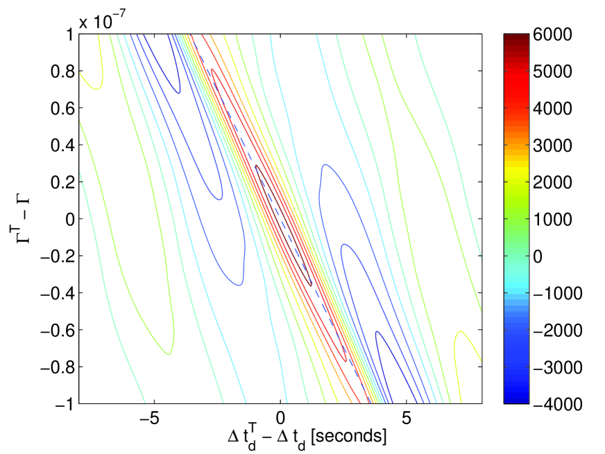
Figure 1: $\zeta$ contour map in the $\Gamma^{T}-\Gamma$ and $\Delta t_{d}^{T}-\Delta t_{d}$ plane, in the absence of noise. The source, lens, and detector parameters are listed in the table LABEL:tbl:Q0957+561. All the template parameters other than $\Gamma^{T}$ and $\Delta t_{d}^{T}$ are fixed to be the right values. The dotted line is Eq. (34), which approximately follows the ridge of $\zeta=\zeta(\Gamma^{T},\Delta t_{d}^{T})$.

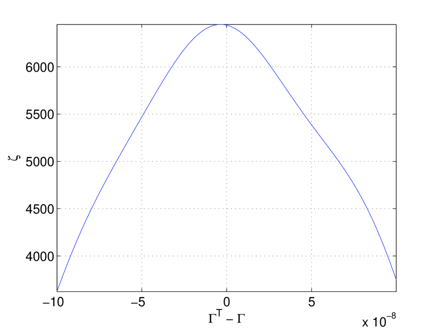
Figure 2: $\zeta$ along the line Eq. (34) projected onto the $\Gamma^{T}-\Gamma$ axis, in the absence of noise. The source, lens, and detector parameters are listed in the table LABEL:tbl:Q0957+561. All the template parameters other than $\Gamma^{T}$ and $\Delta t_{d}^{T}$ are fixed to be the right values.

VII Correlation among the parameters

As is mentioned in Sec. IV, we specifically assume the following situation: Two images occur due to gravitational lensing. A gravitational wave is in the detector’s observation frequency band during the time segment from $t_{s,1}$ to $t_{e,1}$. We use matched filtering technique to estimate the source parameters (8 in the lowest order, Eq. (18)). Another wave reaches the detector from $t_{s,2}=t_{s,1}+\Delta t_{d}$ to $t_{e,2}=t_{e,1}+\Delta t_{d}$, and we use matched filtering technique to estimate the source parameters. From similarity of the estimated values of the parameters, we would conclude that we see gravitational lensing of gravitational waves. We then construct a filter $\Theta(f,{\bf p}^{T})$ from the estimated parameters, compute a filtered cross-correlation $\zeta$, and estimate $\Gamma$ and $\Delta t_{d}$. Therefore, in practice, an estimates of $\Gamma$ and $\Delta t_{d}$ should be affected by errors in estimates of other parameters ${\bf p}^{T}$ in $\Theta(f,{\bf p}^{T})$ (We do not estimate ${\bf p}^{T}$ at the same time as $\Gamma^{T}$ and $\Delta t_{d}$ when computing the filtered cross-correlation).

To find the effect of the errors in ${\bf p}^{T}$ to the estimate of $\Gamma$, we performed the following simulations. We generate a wave with the source parameters ${\bar{\theta}_{L},\bar{\phi}_{L},\bar{\theta}_{S},\bar{\phi}_{S},\phi_{c},\bar{\phi}_{0},\alpha_{0}}$ randomly chosen (and thus we generate waves with randomly chosen ${\bf p}$). Other source parameters are fixed and listed in the table LABEL:tbl:Q0957+561. For each parameters set, we take the template parameters by adding random Gaussian errors $\delta{\bf p}$ to the injected signal parameters ${\bf p}$ as ${\bf p^{T}}={\bf p}+\delta{\bf p}$. The standard deviations of the errors are $10^{-6}$ for the relative errors in the mass $m_{j}$ and the time of coalescence $t_{c}$, and $0.1$ radians for the angular parameters ${\bar{\theta}_{L},\bar{\phi}_{L},\bar{\theta}_{S},\bar{\phi}_{S},\phi_{c},\bar{\phi}_{0},\alpha_{0}}$ Crowder and Cornish (2005). We then compute our statistic $\zeta$ and find $\Gamma$ and $\Delta t_{d}$ that maximize $|\zeta|$. We repeated the above steps 1100 times. Fig. 3 shows the result of the simulation. Here we search over the region of $|\Gamma^{T}-\Gamma|<10^{-7}\cap|\Delta t_{d}^{T}-\Delta t_{d}|<20$ sec (The size of the search region is limited from our computer power). We see the estimates of $\Gamma$ and $\Delta t_{d}$ roughly satisfy Eq. (34). Several points ($8\%$ of all) are accumulated around the upper left and the lower right boundaries of the search region, for which the estimates should in fact be outside of the region. Fig. 4 shows the result of the same simulation but with the true time delay $\Delta t_{d}$ enlarged to $5.1$ years, and correspondingly $f_{i}=0.065$ Hz. We see a better correlation to Eq. (34) and a smaller points accumulated around the boundary of the region ($3\%$). Both of the figures show a tendency that larger the value of $\zeta$ is, better the accuracy of our estimates for $\Gamma$ and $\Delta t_{d}$ are.

Now what are the effect of the errors in the ${\bf p}^{T}$ onto estimates of $\Gamma$ and $\Delta t_{d}$? Fig. 5 and Fig. 6 show the cumulative probabilities of the absolute errors in $|\Gamma^{T}-\Gamma|$ and $|\Delta t_{d}^{T}-\Delta t_{d}|$. From Fig.5, we conclude that errors in ${\bf p}^{T}$ cause errors of less than $2.5\times 10^{-8}$ in $\Gamma^{T}$ ($\Gamma=4.9\times 10^{-8}$) for $35\%$ of the simulation for $\Delta t_{d}=1.14$ years and $70\%$ of the simulation for $\Delta t_{d}=5.1$ years.

Finally, the scatter plot Fig. 7 shows how the errors in $M_{cz}$ and $t_{c}$ affect our estimate of $\Gamma$. Since $M_{cz,1}/M_{cz,2}=\Gamma$, we can determine $\Gamma$ using estimates of $M_{cz,j}$, if this ratio can be determined accurately enough. This figure shows that even though we admit errors in $M_{cz}$ of order $10^{-6}$ (note that the injected signals have $\Gamma=4.9\times 10^{-8}$), $\Gamma$ can be determined at less than $10^{-7}$ accuracy in our simulation, using our filtered cross-correlation method.

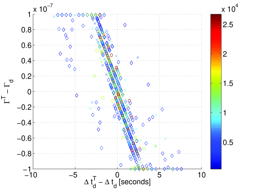
Figure 3: A scatter plot of maximum locations of $\zeta$ in the $\Gamma^{T}-\Gamma$ and $\Delta t_{d}^{T}-\Delta t_{d}$ plane for 1100 sets of randomly chosen source, lens, and detector parameters. Here $\Delta t_{d}=1.14$ years. Symbols indicate $\zeta$ values: $\zeta_{{\rm max}}\sim 2.8\times 10^{4}$ denoting the maximum value of $\zeta$ in the 1100 trials, diamonds for $0\leq\zeta<0.25\zeta_{{\rm max}}$, crosses for $0.25\zeta_{{\rm max}}\leq\zeta<0.5\zeta_{{\rm max}}$, circles for $0.5\zeta_{{\rm max}}\leq\zeta<0.75\zeta_{{\rm max}}$, and squares for $0.75\zeta_{{\rm max}}\leq\zeta\leq\zeta_{{\rm max}}$. See Sec. VII for details.

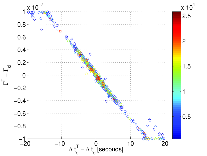
Figure 4: The same as Fig. 3 but here $\Delta t_{d}=5.1$ years and correspondingly $f_{i}=0.065$ Hz. See Sec. VII for details.

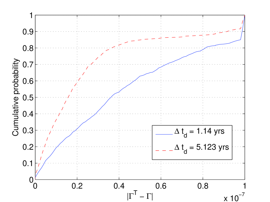
Figure 5: Cumulative probability distributions of $|\Gamma^{T}-\Gamma|$. See Sec. VII for details.

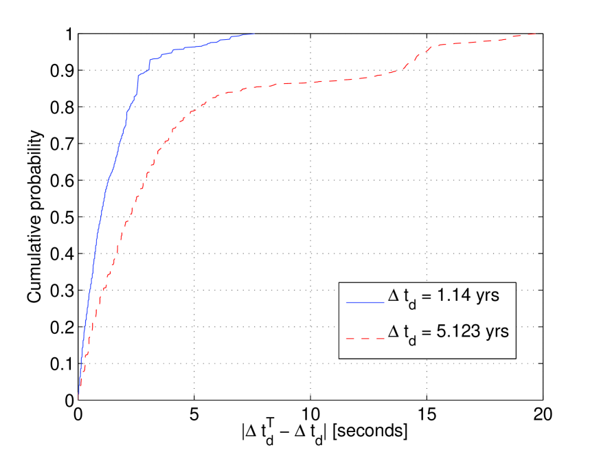
Figure 6: Cumulative probability distributions of $|\Delta t_{d}^{T}-\Delta t_{d}|$. See Sec. VII for details.

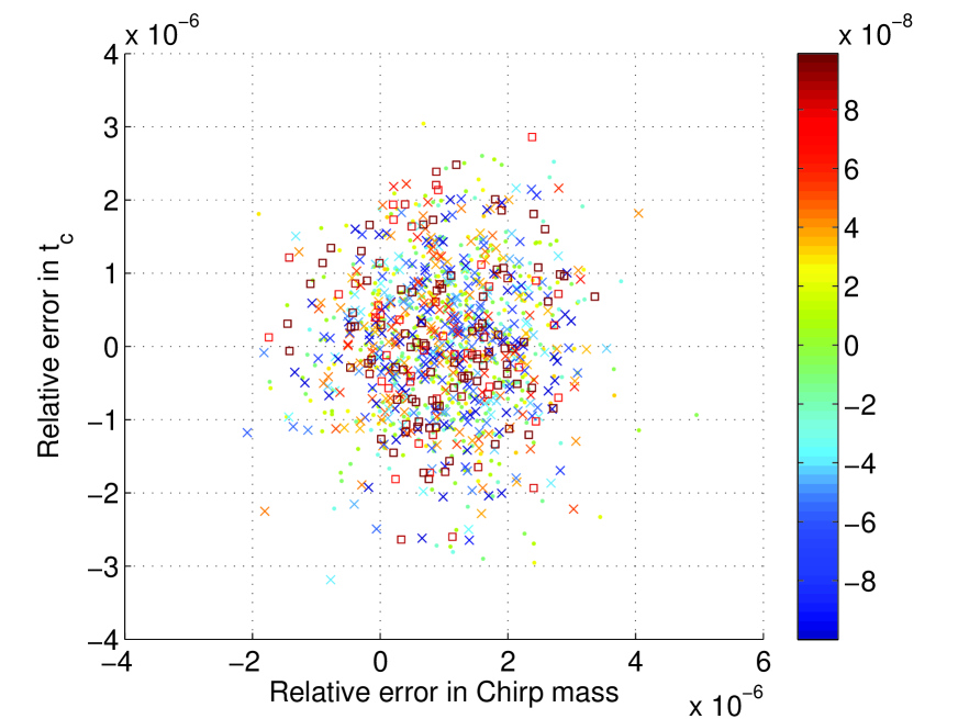
Figure 7: A scatter plot of maximum locations of $\zeta$ in the $M_{cz}^{T}/M_{cz}-1$ and $t_{c}^{T}/t_{c}-1$ plane for 1100 sets of randomly chosen source, lens, and detector parameters. Here $\Delta t_{d}=1.14$ years. Symbols indicate $|\Gamma^{T}-\Gamma|$ values: dots for $0\leq|\Gamma^{T}-\Gamma|<3.33\times 10^{-8}$, crosses for $3.33\times 10^{-8}\leq|\Gamma^{T}-\Gamma|<6.67\times 10^{-8}$, and squares for $6.67\times 10^{-8}\leq|\Gamma^{T}-\Gamma|$. The true value of $\Gamma$ is $4.9\times 10^{-8}$.

VIII Precision to which we could measure $\theta\beta_{\perp}$

In reality, there is a noise in detector’s outputs, so the Eqs. (20) and (21) should be actually

$$s_{A}(t) = \sum_{j=1,2}h_{j}(t)+n_{A}(t)\,\,\,{\rm for}\,\,\,t_{e,1}-\Delta t_{d}\leq t\leq t_{e,1},$$ (36)

$$s_{B}(t) = h_{j=2}(t)+n_{B}(t)\,\,\,{\rm for}\,\,\,t_{e,1}\leq t\leq t_{e,2},$$ (37)

where $n_{k=A,B}(t)$ are the detector’s noise. The presence of noise affects firstly the estimates of the filter parameters ${\bf p}^{T}$ when one use matched filtering to estimate those. Secondly, it affects the estimates of $\Gamma^{T}$ and $\Delta t_{d}^{T}$ when we use a filtered cross-correlation technique. We studied the former effect in the previous section, and here we study the combination of them. In the presence of the noise, $\zeta$ statistic should be

$$\zeta = 4Re\int_{f_{i}}^{f_{e}}\frac{s_{A}(f)s_{B}^{*}(f)}{S_{h}(f)}\cos(2\pi f\Delta\tilde{t}^{T}_{d,1}+\Theta(f,\mathbf{p}^{T}))df$$ (39)

$$= \zeta_{0}+4Re\sum_{\alpha}\int_{f_{i}}^{f_{e}}\frac{n_{A}(f)h_{\alpha,2}^{L*}(f)}{S_{h}(f)}\cos(2\pi f\Delta\tilde{t}^{T}_{d,1}+\Theta(f,\mathbf{p}^{T}))df$$

$$+ 4Re\sum_{\alpha}\int_{f_{i}}^{f_{e}}\frac{n_{B}(f)h_{\alpha,1}^{L*}(f)}{S_{h}(f)}\cos(2\pi f\Delta\tilde{t}^{T}_{d,1}+\Theta(f,\mathbf{p}^{T}))df$$

$$+ 4Re\int_{f_{i}}^{f_{e}}\frac{n_{A}(f)n_{B}^{*}(f)}{S_{h}(f)}\cos(2\pi f\Delta\tilde{t}^{T}_{d,1}+\Theta(f,\mathbf{p}^{T}))df.$$

$\zeta_{0}$ is $\zeta$ statistic without noise given by Eq. (24). As is in the previous section, we first generate a wave with a randomly chosen source parameters set ${\bar{\theta}_{L},\bar{\phi}_{L},\bar{\theta}_{S},\bar{\phi}_{S},\phi_{c},\bar{\phi}_{0},\alpha_{0}}$ where other parameters are taken from the table LABEL:tbl:Q0957+561. We then assume template parameters ${\bf p}^{T}$ by adding Gaussian errors to the true parameters of the generated signal. The standard deviations of the errors are the same as before. For each realization of the wave, we further add random Gaussian noise $n_{j}(f)$ satisfying $<n(f)n^{*}(f^{\prime})>=S_{h}(f)\delta(f-f^{\prime})/2$ where $<...>$ denotes ensemble average. We then compute our statistic $\zeta$ and find $\Gamma$ and $\Delta t_{d}$ that maximize $|\zeta|$. For each generation of a wave, noise frequency series is generated 1000 times. We went through these steps 10 times, so that we obtained total of $10\times 1000$ estimates of $\Gamma$ and $\Delta t_{d}$.

The results of the simulation are as follows. The cumulative probabilities of the errors in $|\Gamma^{T}-{\rm Mean}(\Gamma^{T})|$ are shown for 8 out of 10 waves in Fig. 8 (For the excluded 2 waves the maximum of the $\zeta_{0}$ appears to close to the search region boundary and we could not compute the cumulative probabilities properly). Here ${\rm Mean}(\Gamma^{T})$ for each source parameters set is the mean of $\Gamma^{T}$ over 1000 realizations of the noise series and does not necessarily equals the true value of $\Gamma$, as studied in the previous section. The standard deviation of the errors is $1.9\times 10^{-8}$ and $90\%$ of the time the error is less than $3\times 10^{-8}$ on average of 8 waves. We also performed the same analysis but with $\Delta t_{d}=1.14$ years replaced by $\Delta t_{d}=5.1$ years (so that $f_{i}=0.113$ Hz by $f_{i}=0.065$ Hz). Fig. 9 shows the result for this longer time delay (and thus longer integration time of 5 years). The standard deviation of the errors in this case is $1.1\times 10^{-8}$ and $90\%$ of the time the error is less than $2\times 10^{-8}$ on average of 10 waves.

Finally, we performed the same analysis for $v=1000{\rm km/s}$ or $\Gamma=10^{-7}$, and obtained quantitatively the same results as above. Combining the results in the previous sections, we conclude that $\Gamma^{T}$ would be determined, in our example, with the future (one-triangle) BBO/DECIGO detectors

$$\Gamma^{T}=\Gamma\pm 5.5\times 10^{-8}\pm 1.9\times 10^{-8}$$ (40)

for 1.14 years integration and

$$\Gamma^{T}=\Gamma\pm 2.0\times 10^{-8}\pm 1.1\times 10^{-8}$$ (41)

for 5.1 years integration, where the first error in each equation is due to the errors in the estimates of the filter parameters ${\bf p}$ and the second error comes from the noise terms in the filtered cross-correlation analysis in Eq. (39).

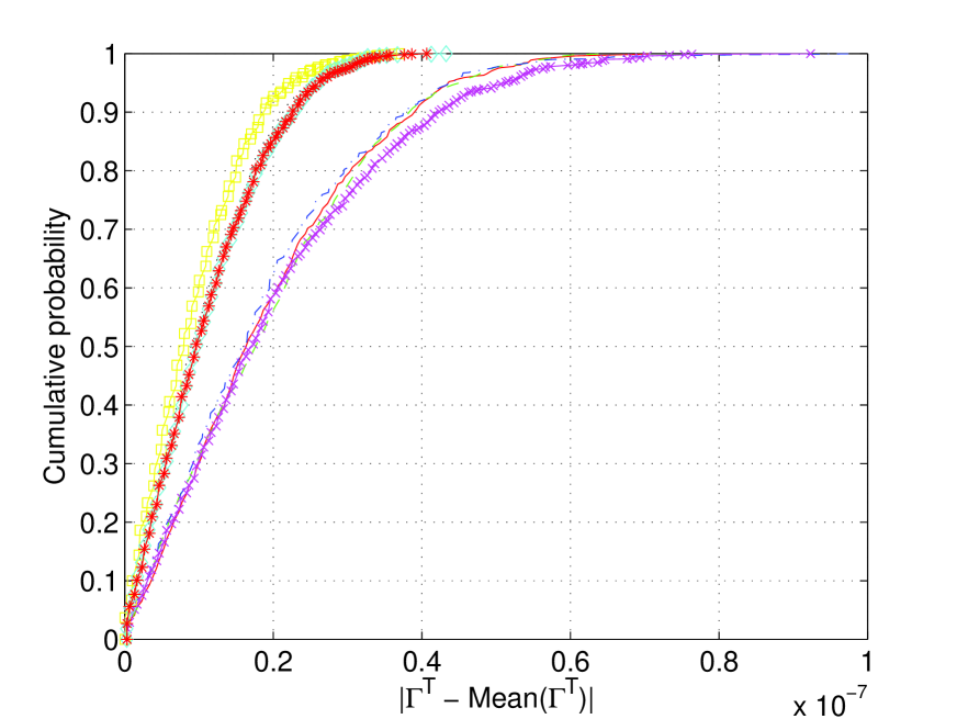
Figure 8: Cumulative probability distributions of $|\Gamma^{T}-{\rm Mean}(\Gamma^{T})|$ for 8 waves with different source-lens-detector parameters sets in the presence of noise. Here $\Delta t_{d}=1.41$ years. See Sec. VIII for details.

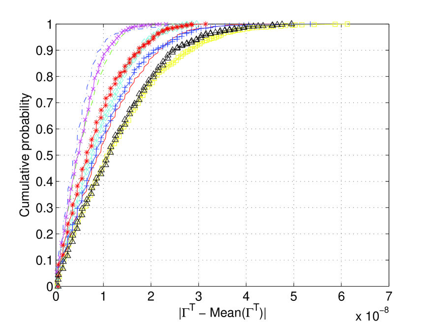
Figure 9: Cumulative probability distributions of $|\Gamma^{T}-{\rm Mean}(\Gamma^{T})|$ for 10 waves with different source-lens-detector parameters sets in the presence of noise. Here $\Delta t_{d}=5.1$ years. See Sec. VIII for details.

IX Summary

In this paper, we considered a gravitational lensing phenomena of gravitational waves in the case when the geometrical optics approximation applies. To be specific, the source was assumed to be a coalescing neutron stars binary at a cosmological distance and a detector to be the planned space-borne detector (one-triangle) BBO/DECIGO. We then proposed a filtered cross-correlation method of extracting the relative transverse velocity of the source-lens-observer system using an interference term.

We performed series of simulations to study correlations among parameters and to estimate errors due to detector’s noise. In these simulations, we adopted lens parameters taken from the lens system Q0957+561 Walsh et al. (1979); Kochanek et al. (2006) as a reference for a demonstration purpose, in which the time delay is $\Delta t_{d}=1.41$ years. With our method, we found the absolute error in $\Gamma=\theta\beta_{\perp}$ ($\theta$ is the images separation and $\beta_{\perp}$ is the relative transverse velocity), with the future (one-triangle) BBO/DECIGO detectors to be $\delta(\Gamma)=\pm 5.5\times 10^{-8}\pm 1.9\times 10^{-8}$ for the time delay of 1.14 years, where the first error in the equation is due to the error in the estimates of the filter parameters ${\bf p}$ and the second error comes from the noise terms in the filtered cross-correlation analysis in Eq. (39). The errors in the equation are the standard deviation estimated in our simulations. We also performed the same analysis but with $\Delta t_{d}=5.1$ years. In this case, we found $\delta(\Gamma)=\pm 2.0\times 10^{-8}\pm 1.1\times 10^{-8}$.

Although the probabilities of lens phenomena is highly uncertain mainly due to the fact that the event rate of neutron stars binaries coalescence is highly uncertain, one observation of transverse velocity of a neutron stars binary may give us valuable information of such population.