Anomalous Thermostat and Intraband Discrete Breathers

Abstract

We investigate the dynamics of a macroscopic system which consists of an anharmonic subsystem embedded in an arbitrary harmonic lattice, including quenched disorder. The coupling between both parts is bilinear. Elimination of the harmonic degrees of freedom leads to a nonlinear Langevin equation with memory kernels $\mathbf{\Gamma}(t)$ and noise term $\bm{\zeta}(t)$ for the anharmonic coordinates $\mathbf{q}(t)={(q_{\alpha}(t))}$. For zero temperature, i.e for $\bm{\zeta}(t)\equiv 0$, we prove that the support of the Fourier transform of $\bm{\Gamma}(t)$ and of the time averaged velocity-velocity correlations functions $\bm{K}(t)$ of the anharmonic system can not overlap. As a consequence, the asymptotic solutions can be constant, periodic, quasiperiodic or almost periodic, and possibly weakly chaotic. For a sinusoidal trajectory $\bm{q}(t)$ with frequency $\Omega$ we find that the energy $E_{T}$ transferred to the harmonic system up to time $T$ is proportional to $T^{\alpha}$. If $\Omega$ equals one of the phonon frequencies $\omega_{\nu}$, it is $\alpha=2$. We prove that there is a zero measure set $\mathcal{L}$ such that for $\Omega$ in its full measure complement $\mathcal{R}\backslash\mathcal{L}$, it is $\alpha=0$, i.e. there is no energy dissipation. Under certain conditions $\mathcal{L}$ contains a subset $\mathcal{L}^{\prime}$ such that for $\Omega\in\mathcal{L}^{\prime}$ the dissipation rate is nonzero and may be subdissipative $(0\leq\alpha<1)$ or superdissipative $(1<\alpha\leq 2)$, compared to ordinary dissipation $(\alpha=1)$. Consequently, the harmonic bath does act as an anomalous thermostat, in variance with the common belief that elimination of a macroscopically large number of degrees of freedom always generates dissipation, forcing convergence to equilibrium. Intraband discrete breathers are such solutions which do not relax. We prove for arbitrary anharmonicity and small but finite coupling that intraband discrete breathers with frequency $\Omega$ exist for all $\Omega$ in a Cantor set $\mathcal{C}(k)$ of finite Lebesgue measure. This is achieved by estimating the contribution of small denominators appearing for $\mathbf{G}(t;\Omega)$, related to $\mathbf{\Gamma}(t)$. For $\Omega\in\mathcal{C}(k)$ the small denominators do not lead to divergencies such that $\mathbf{G}(t;\Omega)$ is a smooth and bounded function in $t$.

Ginwidth=0.7

and

1 Introduction

The analytical treatment of the dynamics of a macroscopic system of $N$ particles is not possible, in general. But there are situations which allow to simplify the dynamical description. We will restrict ourselves to classical systems. One of the prominent examples is Brownian motion. A big particle with mass $M$ interacts with a solvent. If the solvent particles have a mass $m$ much smaller than $M$ a time scale separation exists. Separating the fast motion of the solvent particles from that of the big one, called Brownian particle, a Langevin equation results for the motion of the Brownian particle. The influence of the solvent particles occurs through a friction and a fluctuating force. These two are related to each other by the so-called fluctuation- dissipation theorem of second kind. For a general system with time scale separation, the Mori-Zwanzig projection formalism [1, 2] allows to derive a Langevin equation for the slow variables. If there is a single slow variable $A$, then one gets [1, 2]

$$\frac{d}{dt}A(t)+i\Omega A(t)+\int\limits_{0}^{t}dt^{\prime}\,M(t-t^{\prime})A(t^{\prime})=f(t)$$ (1)

where $\Omega$ is a microscopic frequency, $M(t)$ a memory kernel and $f(t)$ the fluctuating force. Elimination of a macroscopic number of fast degrees of freedom always leads to memory effects. If $M(t)$ relaxes much faster then the average of $A(t)$, one can perform a Markov approximation, i.e. $M(t)\approx 2\gamma\delta(t-t^{\prime})$. The analytical calculation of $M(t)$ is not feasible, in general. However, there exists a class of models for which the exact elimination of a macroscopic number of degrees of freedom is possible, even if there is no time scale separation. These models we call Kac-Zwanzig models [3, 4]. They consist of a subsystem coupled to a macroscopic bath of harmonic oscillators. The subsystem can be microscopic, i.e. the number of its degrees of freedom is of order one or it can also be macroscopic with, e.g. 10²³ degrees of freedom. Since the equations of motion are linear in the oscillator coordinates, the harmonic degrees of freedom can be microscopic, i.e. the number of its degrees of freedom is of order one or it can also be macroscopic with, e.g. 10²³ degrees of freedom. As a result, one obtains for the coordinates of the subsystem a stochastic differential equation of type of eq.(1). The memory kernel $M$ (which is a matrix in general) can be expressed by an integral over the frequencies of the harmonic bath. Its spectral properties strongly influence the time dependence of $M$ and therefore that of the coordinates of the subsystem, too. In the Langevin case where the spectrum is absolutely continuous with infinite support, the subsystem will relax to equilibrium for all of its initial conditions. In this case, the harmonic oscillators act as a normal thermostat. However, if, e.g. that spectrum contains a dense discrete component as it occurs for harmonic systems with quenched disorder, the situation may be different. Then, there exist initial conditions, which will not relax to equilibrium, but may converge to periodic, quasiperiodic or possibly weakly chaotic solutions. This behavior is closely related to the existence of spontaneous energy localization.

Spontaneous energy localization in large nonlinear discrete systems is now known as an ubiquitous phenomena related to the existence of Discrete Breathers (DBs). When a sufficiently large amount of energy is injected locally in a system which may sustain DBs and which is initially at low temperature, it is found that although some part of this energy spreads over the system, a substantial part of this energy may remain localized as a DB [5] over very long time. The discovery of this kind of localized modes was so surprising because they existed in systems with discrete translational invariance in space. DBs also called Intrinsic Localized Modes(ILM) are spatially localized time periodic solutions of discrete nonlinear Hamiltonian systems [6, 7, 8, 9]. Since many of them are linearly stable and thus can trap energy over long times, they should play an essential role in energy relaxation in complex systems.

The existence of DBs has been rigorously proven by several methods and for a variety of models with optical or acoustic phonons, with or without gaps, in one or any dimension and without or with randomness [10, 11, 12, 13, 14]. All these existence proofs require that the DB frequency and its harmonics do not belong to the phonon spectrum (obtained by linearization of the dynamical equations in the vicinity of the ground state). Otherwise, the DB would be expected to radiate energy in the phonon band and to decay. In addition, the proofs [10, 11, 12, 13, 14] only concern the existence of out-of-band DBs, i.e. their frequencies and those of the higher harmonics are in the band gaps of the phonon spectrum. For certain models the existence of DBs was even proven before by Albanèse and Fröhlich [15, 16] and by Albanèse, Fröhlich and Spencer [17] under the requirement of randomness. In that case the eigenstates of the linear eigenvalue problem are already localized (in dimensions larger than two the randomness has to be large enough) and therefore it is more intuitive that localized time periodic solutions could persist in the presence of nonlinearities, although to prove this is highly nontrivial

When the phonon spectrum is discrete, for example in a strongly disordered system with Anderson localization, energy radiation of linear phonons by a localized time periodic solution cannot occur. Then, the existence of Intraband Discrete Breathers (IDBs) with their frequency or some of their harmonics inside the phonon spectrum, might be a priori possible. Indeed, numerical evidence [18, 19] suggested that such solutions do exist. More precisely, it was conjectured that for each localized Anderson mode, there is an associated family of IDBs with variable frequencies (and amplitude), which converges to this Anderson mode at the small amplitude limit. It was also conjectured that the IDBs with respect to their frequency dependence do not form a continuous family of solutions as for ordinary (out-of-band) DBs, but are defined only on a fat Cantor set of frequencies (i.e. with nonvanishing Lebesgue measure). A forbidden frequency gap is associated with each of the other frequencies of the linear Anderson modes. These frequencies are dense in the linear phonon spectrum but the width of these gaps drops to zero very fast as a function of the spatial distance of the corresponding Anderson mode of the center to the IDB. Then, the complementary Cantor set of frequencies where the IDB exists is non void with a strictly positive Lebesgue measure. Moreover, the measure density of this Cantor set is expected to go to full measure when the amplitude of the IDB goes to zero that is when the IDB tends to be a linear mode.

The IDB should not be confused with so-called embedded solitons in discrete lattice systems (see [20, 21] and references therein). These are nonlinear excitations with a discrete frequency lying within the linear spectrum, whereas IDB take frequencies from a set of full measure. Furthermore, in contrast to IDB the existence of embedded solitons requires exponentially localized linear modes.

The first proof of existence of such IDBs for a certain class of random models was done by Albanèse and Fröhlich [15, 16] and by Albanèse, Fröhlich and Spencer [17]. The models studied by these authors are the random, discrete Schrödinger equation and the wave equation with a cubic nonlinearity. A perturbational approach was used to prove that all periodic solutions of the linear equation can be continued for small enough $\lambda$, the strength of nonlinearity. For arbitrary $\lambda$ it was proven that there exist at least certain periodic solutions. Transforming a random, nonlinear dynamical system without acoustic phonons into Anderson space, i.e. to the space of the localized eigenstates of the linear problem and restricting to nearest neighbor interactions in Anderson space, Fröhlich, Spencer and Wayne [22] have even proven (under certain conditions) the existence of localized almost periodic solutions, i.e. of KAM tori.

Besides the existence of IDBs, it was also conjectured in [18, 19] the existence of families of multibreather states which exhibit several energy peaks associated with different Anderson modes. We may explain intuitively this conjecture by the fact that the frequency of a nonlinear mode depends on its amplitude. It is thus possible to tune the amplitude of an arbitrary number of different Anderson modes in order they get the same frequency. Despite nonlinear modes cannot be simply superposed as in the linear case, a time periodic multibreather solution can be constructed numerically. When, the number of IDBs involved in the multibreather state is infinite, these multibreather states are spatially extended and able to transport energy by phase torsion [23]. As a result, nonlinearity restores the ability of the system to transport energy.

The aim of this paper is to provide an exact proof of these conjectures for a special class of random models where the underlying physical arguments appear explicitly. These models, consisting of a microscopic or macroscopic anharmonic subsystem coupled to a bath of harmonic oscillators, are designed on one hand for obtaining simpler mathematical proofs and on the other hand to contain nevertheless the essential features, e.g. for the trajectories $\bm{q}(t)$ of the anharmonic system, which can be found in more general complex and realistic models. Although these results do not provide a rigorous proof (in the mathematical sense) for general and fully anharmonic systems, they nevertheless make clearer the fundamental reasons for their existence and thus support the earlier conjecture that they might exist in general.

Particulary, we will derive for rather general anharmonic and harmonic subsystems(arbitrary dimension, with or without disorder) an exact formula which relates the energy dissipation rate ${\overline{{\dot{E}}_{T}}}$ of the anharmonic system averaged over a time interval of length $T$ to the Fourier transform ${\tilde{\bm{\Gamma}}}(\omega)$ of the dissipation kernels $\bm{\Gamma}(t)$ and to ${\bm{\tilde{K}}}(\omega)$, the Fourier transform of the velocity-velocity correlation functions of the trajectories $\bm{q}(t)$. For finite initial energy and bounded Hamiltonian from below it is ${\overline{\dot{E}}_{T}}\rightarrow 0$ for $T\rightarrow\infty$. This will yield the nonoverlapping criterion for the support of ${\bm{\tilde{\Gamma}}}(\omega)$ and ${\bm{\tilde{K}}}(\omega)$ which will have consequences for the possible asymptotic behavior of $\bm{q}(t)$ for $t\rightarrow\infty$. Calculation of the energy dissipation rate ${\overline{\dot{E}}_{T}}$ for a sinusoidal force with frequency $\Omega$ will demonstrate the existence of extreme sensitivity of the dissipated energy by that force on its frequency $\Omega$. Compared to ordinary dissipation where $E_{T}\sim T$, superdissipative and subdissipative behavior may occur for which $E_{T}$ increases, respectively, faster and slower than $T$. We will also show that there exists a set of full measure such that $E_{T}$ is bounded for all $\Omega$ in that set, i.e. no energy dissipation exists at all.

The possibility of no energy dissipation allows the existence of periodic solutions $\bm{q}(t+2\pi/\Omega)=\bm{q}(t)$, also within the phonon band. We will show that such IDB exist with frequencies on a fat Cantor set. In that case relaxation to equilibrium is prohibited such that the harmonic bath acts as an anomalous thermostat. This behavior is related to the pioneering work of Fermi, Pasta and Ulam, which has given evidence for nonergodic dynamics. New results confirm that ergodicity in phase space of large and complex dynamical systems is not as smooth as it was believed through Langevin bath theory. When starting from initial states which are not at thermal equilibrium, there are many islands in phase space which may trap the state of the system for long time and could result in unusual and slow relaxation processes toward the thermal equilibrium.

2 Modeling the Intraband Discrete Breather Problem

In order to keep our presentation selfcontained we review and discuss properties of linear spectra which have been proven earlier or are well-admitted in order to define a model and an associated set of hypothesis which could match with the different physical situations. Our purpose is to describe the main characteristics which could be expected for large families of nonlinear random models with linear spectrum involving both discrete and continuous components. Continuous spectra occur only in the thermodynamic limit, i.e. for an infinite system.

In order to fix the ideas, let us consider as an example a random model on a d-dimensional hypercubic lattice, for example a Klein-Gordon type model with Hamiltonian

$$\mathcal{H}=\sum_{i}\left(\frac{p_{i}^{2}}{2}+V_{i}(u_{i})\right)+\sum_{\langle i,j\rangle}\frac{C}{2}(u_{i}-u_{j})^{2}$$ (2)

where the momentum $p_{i}$ is the variable conjugate to the displacement $u_{i}$ at site $i$. The local potential $V_{i}(u_{i})$ is random. For example it could have the form

$$V_{i}(u_{i})=\frac{\omega_{i}^{2}}{2}u_{i}^{2}+\frac{\kappa_{3}}{3}u_{i}^{3}+\frac{\kappa_{4}}{4}u_{i}^{4}+...$$ (3)

where $\omega_{i}$ is chosen according to some probability law $P(\omega)$. $\langle i,j\rangle$ denotes the bonds which connect neighboring sites $(i,j)$ (counted once). Accordingly, the sum in eq.(2) is a double sum over all $i$ and $j$ which are nearest neighbors. $C$ is the constant of the harmonic coupling between nearest neighbors, which is assumed to be identical for all nearest neighbor bonds. The dynamical equations are

$$\ddot{u}_{i}+V_{i}^{\prime}(u_{i})+\sum_{j:i}C(u_{j}-u_{i})=0$$ (4)

$j:i$ denotes the sites $j$ which are nearest neighbors to $i$, i.e. the sum in eq.(4) is a single sum over $j$ which are nearest neighbors of $i$. DBs are spatially localized time periodic solutions of eq.(4). Thus, their amplitude must decay to zero at infinity. Consequently, we may approximate this dynamical system by another dynamical one which obeys the same eq.(4) for the few sites $i$ where the amplitudes of the DB is not small and the linearized equations

$$\ddot{u}_{i}+V_{i}^{\prime\prime}(0)u_{i}+\sum_{j:i}C(u_{j}-u_{i})=0$$ (5)

for all the other sites $i$. Thus, the system becomes equivalent to a finite anharmonic system coupled linearly by local interactions to a harmonic system (phonon bath). Note, we start with a finite harmonic system and finally take the thermodynamic limit. For a finite harmonic system the linear spectrum is always discrete.

This kind of approximation strongly simplifies the investigation of DBs. Assuming the existence of time periodic solutions (DBs) of the isolated anharmonic system (i.e. uncoupled with the harmonic phonon bath) we will discuss under which conditions these solutions could persist when the coupling to the phonon bath is non vanishing, although not too large. This harmonic phonon bath considered uncoupled to the anharmonic system, is characterized by its frequency spectrum. When the frequency of the DB and its harmonics do not belong to the frequency spectrum of the phonon bath, the proof that the DB solutions can be continued to nonzero coupling can be obtained as in [10]. This will be performed in the $5.$ section. When the frequency of the DB, one of its harmonics or several belong to the frequency spectrum of the phonon bath, it is essential to consider whether this phonon spectrum is discrete or continuous.

Figs. 1 and 2, respectively, show possible schemes representing situations where the linear phonons are either spatially extended or localized at the DB frequency.

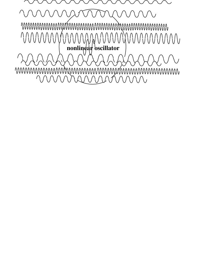
Figure 1: The eigenmodes of the uncoupled phonon bath are extended waves at the DB frequency. Then, at nonvanishing coupling periodic oscillations of the anharmonic system should generate waves which propagate and carry energy at infinity. As a result, the DB solution cannot persist as a finite energy (spatially localized) time periodic solution.

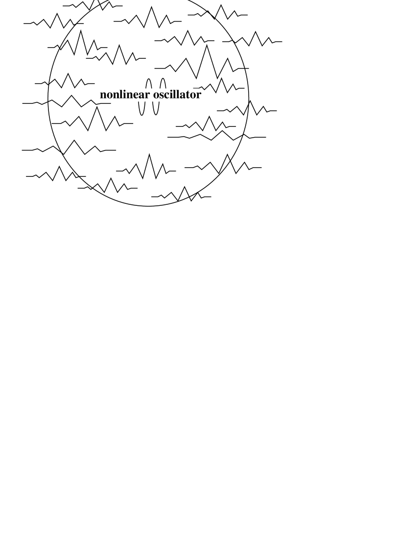
Figure 2: The eigenmodes of the uncoupled phonon bath are spatially localized at the DB frequency. No energy propagation is possible. Then, the DB solution of the anharmonic system may persist at finite coupling.

The model we propose is simply to consider the system as harmonic in the regions where the amplitude of the DB is expected to be small and to keep it anharmonic in the region where the solution has a large amplitude. Of course, our model shall depend on the location of the IDB or multiDBs we consider since it determines the selection of the anharmonic subsystem.

This kind of simplification also allows to investigate the relaxation of an arbitrary localized initial excitation. If the finite initial energy is spread completely over the system the displacements become arbitrary small and the linearization of eq.(4) is allowed for large enough times. However, if the spreading is incomplete, we are allowed to linearize eq.(4) outside the localized region.

When $\{u_{i}\}$ is uniformly small, the linearized equations which yield the linear phonon spectrum are

$$\ddot{\epsilon}_{i}+\omega_{i}^{2}\epsilon_{i}+\sum_{j:i}C(\epsilon_{j}-\epsilon_{i})=0$$ (6)

which has time periodic solutions of the form $\epsilon^{(\alpha)}_{i}(t)=\epsilon^{(\alpha)}_{i}e^{i\omega_{\alpha}t}$. The eigenfrequencies $\omega_{\alpha}$ and eigenmodes $\bm{\epsilon}^{(\alpha)}=\{\epsilon_{i}^{(\alpha)}\}$ obey the eigenequation

$$\left(\mathbf{A_{0}\bm{\epsilon}^{(\alpha)}}\right)_{i}=\omega_{i}^{2}\epsilon_{i}^{(\alpha)}+\sum_{j:i}C(\epsilon_{j}^{(\alpha)}-\epsilon_{i}^{(\alpha)})=\omega_{\alpha}^{2}\epsilon_{i}^{(\alpha)}$$ (7)

where $\mathbf{A}_{0}$ is the matrix of the second order variation of the potential energy from its ground state. The eigenfrequencies $\omega_{\alpha}$ should not be confused with the frequencies $\omega_{i}$ of the small amplitude oscillations in the local potential $V_{i}(u_{i})$.

2.1 Linear Spectrum Properties

It has been proven [24] that the linear spectrum of eq.(7) is discrete and its eigenvectors (Anderson modes) are square summable and exponentially localized with probability one, when either the spatial dimension is less than three or the coupling is not too large. At larger coupling and when the dimension of the lattice is at least three, it is believed that there exist mobility edges in the spectrum (although no rigorous proof is available up to now). There are two mobility edges which determine a central interval where the spectrum is continuous. The corresponding eigenmodes are extended and non square summable. In two intervals limited by the edge of the spectrum, the spectrum is discrete and the corresponding eigenmodes are square summable and exponentially localized.

More generally, we may consider nonlinear models on arbitrary discrete lattices where the small amplitude solution leads to the eigenvalue equation

$$\mathbf{A}\mathbf{x}_{\alpha}=E_{\alpha}\mathbf{x}_{\alpha}$$ (8)

for an arbitrary positive bounded self-adjoint linear operator $\mathbf{A}$ operating in the Hilbert space $\mathbf{x}=\{x_{\mathbf{n}}\}$ where $\mathbf{n}$ represent the sites of an infinite discrete lattice $\mathcal{L}$ in $1,2,3...$ dimensions (or any discrete network), with the standard Hermitian product $\langle\mathbf{x}|\mathbf{y}\rangle=\sum_{\mathbf{n}}x_{\mathbf{n}}^{*}y_{\mathbf{n}}$ and $||\mathbf{x}||=(\langle\mathbf{x}|\mathbf{x}\rangle)^{1/2}$. Since we consider physical systems which have to be linearly stable, we must assume the spectrum to be positive or zero and then, the eigenvalues $E_{\alpha}=\omega_{\alpha}^{2}$ are the square of the eigenmode frequencies. We may also consider systems with acoustic phonons where the spectrum is gapless and contains the translation mode $x_{\mathbf{n}}\equiv a$ associated with zero eigenfrequency which is always extended.

Standard mathematical theories decompose the spectrum $\mathcal{S}$ of such a self-adjoint bounded linear operator $\mathbf{A}$ in three parts: the absolutely continuous spectrum, the discrete spectrum and the singular continuous spectrum [25]. The characteristics of the spectrum manifests itself in finite size systems in the limit of large size $N$ as explained now. The eigenvalue equation restricted to a finite subset $\mathcal{N}$ of $N$ indices of $\mathcal{L}$ corresponds to the diagonalization of a finite self-adjoint matrix

$$\mathbf{A}^{(\mathcal{N})}\mathbf{x}_{\alpha}^{(\mathcal{N})}=E_{\alpha}^{(\mathcal{N})}\mathbf{x}_{\alpha}^{(\mathcal{N})}$$ (9)

which yields $N$ orthogonal and normalized eigensolutions $\mathbf{x}_{\alpha}^{(\mathcal{N})}$ with compact support $\mathcal{N}$ corresponding to real eigenvalues. Taking $N\rightarrow+\infty$ such that the finite support tends to cover the infinite lattice $\mathcal{N}\rightarrow\mathcal{L}$, the nonvanishing accumulation points for the weak topology $\mathbf{x}_{\alpha}$ of the eigensolutions of finite systems $\mathbf{x}_{\alpha}^{(\mathcal{N})}$ are eigensolutions of eq.(8) for an eigenvalue $E_{\alpha}$, the corresponding limit of $E_{\alpha}^{(\mathcal{N})}$. The nonvanishing limit solutions are necessarily square summable with a nonzero norm smaller or equal to $\|\mathbf{x}_{\alpha}^{(\mathcal{N})}\|=1$ and thus can be normalized.

This set of square summable eigensolutions $\mathbf{x}_{\alpha}$ with eigenvalues $E_{\alpha}$ determines the discrete spectrum of $\mathbf{A}$. Since $\mathcal{L}$ is countable, the discrete set of normalized eigenvectors is also countable (or finite). The inverse rate of the exponential decay of the eigenmodes determines the so called localization length which is a smooth function of the eigenfrequency and diverges when approaching mobility edges. In systems with acoustic phonons in 3 dimensions and more, it is believed that the spectrum becomes continuous in a nonvanishing positive interval close to zero and then there is only one mobility edge.

Extended states (e.g. plane waves) are not square summable and their norm diverges proportionally to the system size $N$. These eigenstates can be nevertheless obtained as nonvanishing accumulations points of $\sqrt{N}\mathbf{x}_{\alpha}^{(\mathcal{N})}$. This set of nonsquare summable solutions and their corresponding eigenvalues of the eigenvalue equation (8) are usually called pseudo eigensolutions and pseudo eigenvalues. They corresponds to the absolutely continuous spectrum of $\mathbf{A}$. They form uncountable continua.

The limits of the other finite size eigenstates which behave spatially differently for example which develop a fractal structure at large scale or which exhibit algebraic decay at infinity, determine the remaining part of the spectrum which is the singular continuous spectrum of $\mathbf{A}$. Although there are examples of operators with purely singular continuous spectrum (for example with quasiperiodic potentials), their contribution to the spectrum of most operators is expected to be marginal, generally, and then it reduces to few isolated specific points of the spectrum (corresponding to the mobility edges).

The spectrum of an operator $\mathbf{A}$ (for example random) is a closed subset $\mathcal{S}$ of the real axis. It might be purely absolutely continuous (for example for operators with spatial periodicity) or purely discrete (for example for operators in 1d with randomness or higher dimension with strong disorder) or it might decompose into two disconnected subsets $\mathcal{S}_{d}$ and $\mathcal{S}_{ac}$ where the spectrum is discrete and absolutely continuous, respectively, separated by mobility edges. This situation is supposed to occur for random operators in 3 dimensions and more at weak enough disorder[19].

2.2 The anticontinuous Limit

Considering now again, the nonlinear system (4) at the anticontinuous limit $C=0$, it simply becomes a collection of uncoupled nonlinear oscillators with Hamiltonian $H_{i}=\frac{p_{i}^{2}}{2}+V_{i}(u_{i})$ and thus is trivially integrable. It is then convenient to represent each anharmonic oscillator with the standard action-angle variables $I_{i},\theta_{i}$. Then, the local Hamiltonian $H_{i}(I_{i})$ is only a function of its action $I_{i}$, and its frequency is $H^{\prime}_{i}(I_{i})=\omega_{i}(I_{i})$. Note, that $\omega_{i}(I_{i})$ should not be confused with the frequencies $\omega_{i}$ in eq.(3). Time periodic solutions at frequency $\Omega$ are obtained by choosing each oscillator $i$ either at rest or oscillating at frequency $\Omega=\omega_{i}(I_{i})$ if there exists $I_{i}$ such that this equality may be fulfilled. The solution corresponding to a Discrete Breather at site $i$ and at frequency $\Omega$ is obtained by choosing all the oscillators $j\neq i$ at rest, except oscillator $i$ which is oscillating at frequency $\Omega$.

At $C=0$, the linear spectrum of eigenfrequencies defined by eq.(7) is the closure $\mathcal{S}_{L}=\overline{\bigcup_{i}\{\omega_{i}\}}$ of the set of linear frequencies. Considering a DB solution at the anticontinuous limit at site $i$ and at a frequency $\Omega$ which is nonresonant with the linear spectrum (that is $p\Omega\notin\mathcal{S}_{L}$ for any integer $p$), and fulfills the condition that $d\omega_{i}(I_{i})/dI_{i}=H^{\prime\prime}_{i}(I_{i})\neq 0$ at $\omega_{i}(I_{i})=\Omega$, it was proven by the implicit function theorem [10], that this solution can be continued as a spatially localized solution for $C\neq 0$ belonging to a nonvanishing interval.

When $\Omega\in\mathcal{S}_{L}$, the proof for the DB existence given in [10] which requires the invertibility of $\mathbf{A}_{0}-\Omega^{2}\mathbf{1}$ breaks down. However, numerical investigations suggested the existence of stable IDBs with frequency $\Omega\in\mathcal{S}_{L}$ although they are not continuous functions of the model parameters. Otherwise, this numerical work also suggested the existence of intraband multisite breathers called multibreathers. A direct proof of existence of IDB in fully anharmonic models is likely possible (as an extension of the present work) but it should be more complex for technical reasons than in the simplified model we propose. We think, however, that this model captures the essential physical features of general nonlinear random models.

2.3 Defining a model for IDBs

We denote by $\mathbf{q}=\{q_{\alpha}\}$ the set of variables which describe the coupled anharmonic oscillators and by $\mathbf{p}$ their conjugate variables. This subsystem is described by an anharmonic Hamiltonian

$$\mathcal{H}_{0}(\mathbf{p},\mathbf{q})=\frac{1}{2}\mathbf{p}^{2}+V(\mathbf{q})$$ (10)

Without restricting generality the masses are chosen to be equal to one. The single anharmonic oscillator where $\mathbf{q}$ is a scalar, is the simplest but a special case. This anharmonic part is linearly coupled to an infinite harmonic system described by the set of variables $\bm{u}=\{u_{i}\}$ and conjugate momenta $\bm{p}=\{p_{i}\}$ where the indices $i$ are nodes of an arbitrary network. The harmonic Hamiltonian is $\mathcal{H}_{\rm harm}(\{u_{i},p_{i}\})=\frac{1}{2}\bm{p}^{2}+\frac{1}{2}\bm{u}^{t}\bm{M}\bm{u}$ where $\bm{M}$ is a bounded self-adjoint operator and $t$ denotes transposition. Again, the masses can be taken equal to unity without lack of generality. The total Hamiltonian takes the form

$$\mathcal{H}=\mathcal{H}_{0}(\mathbf{p},\mathbf{q})+\mathcal{H}_{\rm harm}(\{u_{i},p_{i}\})-\lambda\mathbf{q}^{t}\mathbf{C}\bm{u}$$ (11)

where the matrix of coupling constants is $\mathbf{C}=\{C_{\alpha,i}\}$ and $\lambda$ is introducted for convenience. These coupling constants are short ranged that is $\sum_{i}|C_{\alpha,i}|^{2}<+\infty$.

It is more convenient to describe the harmonic system as a collection of noninteracting harmonic oscillators $\nu$ which corresponds to its normal modes. The normal mode coordinates of the harmonic oscillators of the phonon bath are now the coefficients $u_{\nu}$ of the expansion of $\{u_{i}\}$ with respect to the normalized eigenmodes $\bm{u}^{(\nu)}$ with frequency $\omega_{\nu}$ which fulfills $\bm{M}\bm{u}^{(\nu)}=\omega_{\nu}^{2}\bm{u}^{(\nu)}$. They are now coupled to the anharmonic system by the set of coefficients $\mathbf{C}_{\nu}=\bm{u}^{(\nu)t}\bm{C}$ or explicitly $C_{\nu,\alpha}=\sum\limits_{i}u^{(\nu)}_{i}C_{\alpha,i}$.

As we assumed above, the set of coupling constants $\mathbf{C_{i}}=(C_{\mathbf{\alpha},i})$ between $\mathbf{q}$ and $u_{i}$ are short ranged. In most physical situations, they decay exponentially, that is there exists two positive constants $K$ and $\gamma$ such that

$$|\mathbf{C}_{\mathbf{i}}|<Ke^{-\gamma|\mathbf{i}|}\quad.$$ (12)

Thus, we may assume the stronger $\textit{L}_{1}$ condition $\sum_{\mathbf{i}}|\mathbf{C}_{i}|<+\infty$ without loosing much generality.

Then, we obtain a total Hamiltonian of the form

$$\mathcal{H}=\mathcal{H}_{0}(\mathbf{p},\mathbf{q})-\lambda\sum_{\nu}\mathbf{C}_{\nu}^{t}\mathbf{q}~{}u_{\nu}+\sum_{\nu}\left(\frac{1}{2}\dot{u}_{\nu}^{2}+\frac{1}{2}\omega_{\nu}^{2}u_{\nu}^{2}\right)\quad.$$ (13)

The reorganization energy $\mathcal{H}_{R}$ is the change in the groundstate energy of the whole system under the constraint of a static displacement $\bm{q}$ of the anharmonic oscillators. It is obtained by minimizing the last two terms of the energy (13) with respect to $u_{\nu}$ for fixed $\mathbf{q}$. This readily yields $\mathcal{H}_{R}(\mathbf{q})=-\frac{\lambda^{2}}{2}\mathbf{q}^{t}\mathbf{K}_{R}\,\mathbf{q}$ where

$$K_{\alpha,\beta}^{(R)}=\sum_{\nu}\frac{C_{\nu,\alpha}C_{\nu,\beta}}{\omega_{\nu}^{2}}<+\infty\quad.$$ (14)

In well-behaved physical models, this sum is always finite since any finite static displacement $\mathbf{q}$ should involve a finite reorganization energy (and a finite force). This condition requires the assumption that the positive definite series ((14)) is always absolutely convergent. For example, the case of models with acoustic modes where one of the $\omega_{\nu}$ may vanish because there is always a mode at zero frequency (which corresponds to the free motion of the “center of mass” of the whole system). This feature may cause a divergency for coefficients of series (14). But in the limit of low frequency, these (acoustic) phonon modes decouple from the local degree of freedom describing the anharmonic part of the system ($\lim_{\omega_{\nu}\rightarrow 0}\mathbf{C}_{\nu}=0$) and thus this reorganization energy (14) remains finite since $\bm{C}_{\nu}$ is linear or even of higher order in $\omega_{\nu}$ for $\omega_{\nu}\rightarrow 0$. The reorganization energy $\mathcal{H}_{R}$ renormalizes the potential energy of the anharmonic subsystem, i.e. we can introduce an effective energy $\mathcal{H}_{eff}(\mathbf{p},\mathbf{q})=\mathcal{H}_{0}(\mathbf{p},\mathbf{q})+\mathcal{H}_{R}(\mathbf{q})$. Thus, the total Hamiltonian (13) may be written as

$$\mathcal{H}=\mathcal{H}_{eff}(\mathbf{p},\mathbf{q})+\sum_{\nu}\left(\frac{1}{2}\dot{u}_{\nu}^{2}+\frac{1}{2}\omega_{\nu}^{2}(u_{\nu}-\frac{\lambda\bm{C}^{t}_{\nu}\bm{q}}{\omega_{\nu}^{2}})^{2}\right)\quad,$$ (15)

where $u_{\nu}(\mathbf{q})=\lambda\mathbf{C}_{\nu}^{t}\mathbf{q}/\omega_{\nu}^{2}$ is the harmonic displacement minimizing the last two terms of (13), for fixed $\mathbf{q}$. Since we did not specify properties of the harmonic subsystem, which is considered as very general, it is now necessary to introduce some assumptions at this level for ensuring our model to be physically realistic. The density of the positive eigenfrequencies $\omega_{\nu}$ of the harmonic bath (called density of states) is the limit of the positive measure defined as

$$d\mu(\omega)=\lim_{N\rightarrow+\infty}\frac{1}{N}\sum_{\nu}\delta(\omega-\omega_{\nu})d\omega$$

In physical situations, it is generally an absolutely continuous measure, dense on a finite interval (that is $d\mu(\omega)=g(\omega)d\omega$ where $g(\omega)$ is a measurable positive function). But this assumption is not necessary and moreover does not characterize whether the phonon spectrum is discrete or continuous.

For example, in spatially periodic harmonic systems the whole phonon spectrum is absolutely continuous with extended eigenstates which are planewaves. In random Anderson models in three dimensions and at weak enough disorder, the phonon spectrum $\mathcal{S}$ may split into two disconnected sets $\mathcal{S}=\overline{\mathcal{S}_{ac}\bigcup\mathcal{S}_{d}}$ which consists of a central interval $\mathcal{S}_{ac}$ where the spectrum is supposed to be absolutely continuous (corresponding to extended eigenstates) and the union $\mathcal{S}_{d}$ of two side intervals where the spectrum is supposed to be discrete (and corresponding to square summable eigenstates). These intervals are separated by mobility edges (isolated points). At large disorder in 3d or at lower dimension for any disorder, the whole spectrum is discrete and consists of a single interval $\mathcal{S}_{d}$.

Actually, in all these examples, the density of states is an absolutely continuous measure which does not determine a priori whether or not the phonon spectrum is continuous or discrete. Note also that in the case of random potentials, the density of states depends only on the statistical properties of the potential and not on the realizations. The characteristics of the spectrum (absolutely continuous, singular continuous or discrete) appears in our model through the properties of the distribution of coupling constants $\mathbf{C}_{\nu}$. They determine the properties of the kernel which appears after elimination of the harmonic variables and which shall be discussed later.

3 Extended Langevin Theory

Models for an anharmonic system coupled to a harmonic phonon bath are ubiquitous in physics for describing relaxation processes, for example chemical reactions within Kramers theory [4, 26]. However, in those applications the spectrum of the harmonic bath was always assumed to be absolutely continuous. In that case, standard calculations yield after elimination of the phonon bath variables, extra damping terms for the anharmonic system (plus Langevin random forces, if the temperature is not zero). When there is a discrete spectrum, the results are totally different, as we shall see now.

The well-known advantage of a coupling with a harmonic phonon bath is that it is straightforward to eliminate the variables of the phonon bath in order to get effective equations for the anharmonic variables [4] (we already took advantage of such a situation for proving the existence of (interband) Discrete Breathers in systems with acoustic phonons [12]).

3.1 Derivation of a Langevin Equation

Making use of eqs. (10) and (13), the dynamical equations are

$$\ddot{\mathbf{q}}+V^{\prime}(\mathbf{q})-\lambda\sum_{\nu}\mathbf{C}_{\nu}u_{\nu} = 0$$ (16)

$$\ddot{u}_{\nu}+\omega_{\nu}^{2}u_{\nu}-\lambda\mathbf{C}_{\nu}^{t}\mathbf{q} = 0$$ (17)

where $V^{\prime}(\mathbf{q})$ stands for the gradient of $V$ with respect to $\mathbf{q}$. The second equation is linear and readily yields

$$u_{\nu}(t)=u_{\nu}^{(0)}(t)+\lambda\frac{1}{\omega_{\nu}}\cdot\int\limits_{0}^{t}\sin{\omega_{\nu}(t-\tau)}~{}\mathbf{C}_{\nu}^{t}\mathbf{q}(\tau)\,d\tau$$ (18)

where

$$u_{\nu}^{(0)}(t)=\left[\frac{\lambda}{\omega_{\nu}^{2}}\mathbf{C}_{\nu}^{t}\mathbf{q}(0)+\epsilon_{\nu}(0)\right]\cos{\omega_{\nu}t}+\frac{\dot{\epsilon}_{\nu}(0)}{\omega_{\nu}}\sin{\omega_{\nu}t}$$

is an arbitrary solution of the homogeneous part of eq.(17) . If we assume the phonon bath in thermal equilibrium, $\epsilon_{\nu}^{(0)}(t)$ is a random variable due to thermal fluctuations and we have at temperature $T$, $\langle\epsilon_{\nu}^{(0)}(0)\epsilon_{\nu}^{(0)}(t)\rangle=\frac{k_{B}{T}}{\omega_{\nu}^{2}}\cos\omega_{\nu}t$. Substituting $u_{\nu}(t)$ from (18) into (16), we obtain

$$\ddot{\mathbf{q}}(t)+V^{\prime}(\mathbf{q}(t))-\lambda^{2}\int\limits_{0}^{t}\mathbf{G}(t-\tau)\mathbf{q}(\tau)\,d\tau-\lambda^{2}\sum_{\nu}\mathbf{C}_{\nu}(\mathbf{C}_{\nu}^{t}\mathbf{q}(0))\cos\omega_{\nu}t-\lambda\bm{\zeta}(t)=0$$ (19)

where the coefficients $G_{\alpha,\beta}(t)$ of matrix $\mathbf{G}(t)$ are defined by

$$G_{\alpha,\beta}(t)=\sum_{\nu}\frac{C_{\nu,\alpha}C_{\nu,\beta}}{\omega_{\nu}}\sin\omega_{\nu}t$$ (20)

This series is absolutely convergent and yields a smooth function of $t$ because of hypothesis (14) and $\omega_{\nu}<\omega_{c}<\infty$:

$$\sum_{\nu}\frac{|C_{\nu,\alpha}C_{\nu,\beta}|}{\omega_{\nu}}<\omega_{c}\sum_{\nu}\frac{\mathbf{C}_{\nu}^{2}}{\omega_{\nu}^{2}}<+\infty$$

$\bm{\zeta}(t)$ is the Langevin random force

$$\bm{\zeta}(t)=\sum_{\nu}\epsilon_{\nu}^{(0)}(t)\mathbf{C}_{\nu}$$ (21)

It is convenient to rewrite eq.(19) as

$$\ddot{\mathbf{q}}(t)+V_{eff}^{\prime}(\mathbf{q}(t))+\lambda^{2}\int\limits_{0}^{t}\mathbf{\Gamma}(t-\tau)\mathbf{\dot{q}}(\tau)\,d\tau-\lambda\bm{\zeta}(t)=0$$ (22)

where

$$V_{eff}(\bm{q}) = V(\bm{q})-\frac{1}{2}\lambda^{2}\sum_{\alpha,\beta}\Gamma_{\alpha,\beta}(0)q_{\alpha}q_{\beta}$$ (23)

$$\Gamma_{\alpha,\beta}(t) = \sum_{\nu}\frac{C_{\nu,\alpha}C_{\nu,\beta}}{\omega_{\nu}^{2}}\cos\omega_{\nu}t$$ (24)

and $d\mathbf{\Gamma}(t)/dt=-\mathbf{G}(t)$. We note $\mathbf{\Gamma}(0)=\mathbf{K}_{R}$ which corresponds to the coefficients of the reorganization energy (14). Eq.(22) has the form of the Langevin equation (1), however with the nonlinear term $V_{eff}^{\prime}(\bm{q}(t))$.

The damping kernel $\mathbf{\Gamma}(t)$ is related to the random force $\bm{\zeta}(t)$ by the general Langevin relation

$$\langle\zeta_{\alpha}(0)\zeta_{\beta}(t)\rangle=k_{B}T\sum_{\nu}\frac{C_{\nu,\alpha}C_{\nu,\beta}}{\omega_{\nu}^{2}}\cos\omega_{\nu}t=k_{B}T\Gamma_{\alpha,\beta}(t)$$ (25)

where $\langle\quad\rangle$ denotes the canonical average with respect to $\{\varepsilon_{\nu}(0)\}$ and $\{\dot{\varepsilon}_{\nu}(0)\}$.

Definition (24) shows that the damping kernel $\mathbf{\Gamma}(t)=\int\bm{\tilde{\Gamma}}(\omega)e^{i\omega t}d\omega$ is the Fourier transform of $\bm{\tilde{\Gamma}}(\omega)$ with matrix elements which are measures

$$\tilde{\Gamma}_{\alpha,\beta}(\omega)d\omega=d\sigma_{\alpha,\beta}(\omega)=\pi\sum_{\nu}\frac{C_{\nu,\alpha}C_{\nu,\beta}}{\omega_{\nu}^{2}}(\delta(\omega-\omega_{\nu})+\delta(\omega+\omega_{\nu}))d\omega$$ (26)

Actually, measure $\sigma_{\alpha,\beta}(\omega)$ may be written in a more compact way as the result of an integration in the complex plane

$$\sigma_{\alpha,\beta}(\omega)=\int_{0}^{\omega}d\sigma_{\alpha,\beta}(\omega^{\prime})=\frac{1}{2}\frac{1}{2\pi i}\oint_{\mathcal{C}(\omega)}<\bm{C}_{\alpha}|\frac{1}{\bm{M}(z-\bm{M})}|\bm{C}_{\beta}>dz$$ (27)

on a closed contour $\mathcal{C}(\omega)$ which encompasses the part of the spectrum of the positive linear phonon operator $\bm{M}$ on the real axis which is smaller than $\omega^{2}$. Here it is $\bm{C}_{\alpha}=(C_{\alpha,i})$. Note that in the case of random potentials, this measure does depend on the realization of the disorder unlike the density of states. This positive measure $d\sigma_{\alpha,\beta}(\omega)$ can be split into three components which are respectively absolutely continuous, discrete and singular continuous measures. eq.(27) proves that this decomposition precisely corresponds to the decomposition of the spectrum $\mathcal{S}$ of operator $\bm{M}$ which describes the phonon bath, into its absolutely continuous $\mathcal{S}_{ac}$, discrete $\mathcal{S}_{d}$ and singular continuous parts $\mathcal{S}_{sc}$. Thus, the support of each of these measure components on the real $\omega$ axis is independent of $\alpha$ and $\beta$. Consequently, the properties of the Fourier transform measure of the memory kernel $\bm{\tilde{\Gamma}}(\omega)$ are directly related to the spectral properties of the phonon bath.

3.2 Relation between Phonon Spectrum and Kernel Properties

We now show how the properties of the kernel $\bm{\Gamma}(t)$ and of its Fourier transform $\bm{\tilde{\Gamma}}(\omega)$ are related to the properties of the phonon bath. Actually, the Fourier transform eq.(26) of the kernel $\bm{\Gamma}(t)$ is not a priori a smooth function but is a positive measure $\bm{\tilde{\Gamma}}(\omega)d\omega$ which very generally can be decomposed into three parts: the absolutely continuous part $\bm{\tilde{\Gamma}}_{ac}(\omega)$ where $\bm{\tilde{\Gamma}}_{ac}(\omega)$ is a positive measurable function of $\omega$. The discrete part $\bm{\tilde{\Gamma}}_{d}(\omega)$ which is a sum of Dirac functions, and the singular continuous part $\bm{\tilde{\Gamma}}_{sc}(\omega)$ is simply the rest. These different components are directly related to the corresponding components of the spectrum of the phonon bath. We will discuss this relationship only qualitatively, without attempting any rigor. The decomposition of the positive measure $\bm{\tilde{\Gamma}}(\omega)d\omega$ into these three parts implies a corresponding decomposition $\mathbf{\Gamma}(t)=\mathbf{\Gamma}_{ac}(t)+\mathbf{\Gamma}_{d}(t)+\mathbf{\Gamma}_{sc}(t)$.Their qualitative time dependence will be discussed below for the absolutely continuous and the discrete part.

• Absolutely Continuous Phonon spectrum
  

  For the eigenvalues $\omega_{\nu}\in\mathcal{S}_{ac}$ which belong to the absolutely continuous part of the phonon spectrum, the eigenvectors $\bm{u}^{(\nu)}$ corresponding to $\omega_{\nu}$ are extended, their components $u_{\mathbf{i}}^{(\nu)}$ of the normalized state are proportional to $1/\sqrt{N}$ where $N$ is the number of sites $i$ of the harmonic part of our system which is supposed to go to infinity. Since we assumed that the coupling with the phonon bath $\mathbf{C}_{i}$ is local that is (12) is fulfilled, we can write

  $$\mathbf{C}_{\nu}\sim\frac{\mathbf{c}_{\nu}}{\sqrt{N}}$$ (28)

  where $\mathbf{c}_{\nu}$ is a finite number independent on $N$ for $N\rightarrow\infty$. Moreover, the extended eigenvector $\bm{u}^{(\nu)}$ and consequently $\mathbf{c}_{\nu}$, depend on a continuous parameter (for example the wave vector). An important consequence is that the average of $\mathbf{c}_{\nu}$ for $\omega_{\nu}\in[\omega-\delta\omega,\omega+\delta\omega]$ in the limit of an infinite system and small $\delta\omega$ is a well-defined measurable function of $\omega$

  $$\langle\mathbf{c}_{\nu}\rangle_{\omega_{\nu}=\omega}=\mathbf{c}(\omega)=(c_{\alpha}(\omega))\quad.$$ (29)

  Thus, the contribution of the absolutely continuous phonon spectrum to the Fourier transform eq.(26) of the Kernel $\bm{\tilde{\Gamma}}(\omega)d\omega$ is nothing but its absolutely continuous part $\bm{\tilde{\Gamma}}_{ac}(\omega)$. If $\mu(\omega)$ is the density of states of the absolutely continuous phonon spectrum the absolutely continuous measure is given by

  $$\tilde{\Gamma}_{\alpha,\beta}^{(ac)}(\omega)d\omega=\frac{c_{\alpha}(\omega)c_{\beta}(\omega)}{\omega^{2}}\mu(\omega)d\omega$$ (30)

  
  

  which implies

  $$\Gamma_{\alpha,\beta}^{(ac)}(t)=\Gamma_{\alpha,\beta}^{(ac)}(-t)=\int_{\omega\in\mathcal{S}_{ac}}\frac{c_{\alpha}(\omega)c_{\beta}(\omega)}{\omega^{2}}\cos(\omega t)\mu(\omega)d\omega.$$ (31)

  
  

  Since $\mu(\omega)$ is absolutely integrable, $\mathbf{\Gamma}_{ac}(t)$ decays as $1/t$ or faster, due to the Riemann-Lebesgue lemma. This holds e.g. for a spatially periodic system in any dimension and for a three- or higher-dimensional system with disorder which is not too strong.
  

• Discrete Phonon Spectrum
  

  For the eigenvalues $\omega_{\nu}\in\mathcal{S}_{d}$ which belong to the discrete part of the phonon bath, $\bm{u}^{(\nu)}$ is a localized square summable eigenmode. Then, the scalar product $\mathbf{C}_{\nu}=\bm{u}^{(\nu)t}\bm{C}$ is finite. Considering an arbitrary closed interval $\mathcal{I}_{d}\subset\mathcal{S}_{d}$, we require a stronger convergence than (14) for the discrete case:

  $$\sum_{\omega_{\nu}\in\mathcal{I}_{d}}\frac{|\mathbf{C}_{\nu}|}{\omega_{\nu}}=B(\mathcal{I}_{d})<+\infty\quad.$$ (32)

  
  

  Actually, this assumption should be fulfilled in most realistic physical situations with a discrete spectrum.
  

  Generally, the eigenmodes $\bm{u}^{(\nu)}$ decay exponentially with respect to $|i|$ and there is a uniform bound on the localization length provided $\omega_{\nu}\in\mathcal{I}_{d}$ (provided this interval does not contain the mobility edges). If we assume the coupling constants $\mathbf{C}_{\mathbf{i}}$ fulfill (12), then $|\mathbf{C}_{\nu}|=|\bm{u}^{(\nu)t}\bm{C}|$ decays exponentially as a function of $d_{\nu}$, the distance from the “center of mass” of mode $\nu$. Then, since $\omega_{\nu}$ is bounded from below by a positive nonvanishing number, series (32) converges. Note, however, that even for a system with acoustic phonons the series (32) may exist because the translational invariance implies at least $\mathbf{C}_{\nu}\sim\omega_{\nu}$ for $\omega_{\nu}\rightarrow 0.$ However, in principle, there is no need for exponential localization, the eigenmodes could decay with some algebraic law providing they are square summable.
  

  The contribution of the discrete spectrum of the phonon bath to the Fourier transform measure (26) is nothing but the discrete part $\bm{\tilde{\Gamma}}_{d}(\omega)$ which is a sum of Dirac functions
  

  $$\tilde{\Gamma}_{\alpha,\beta}^{(d)}(\omega)d\omega=\pi\sum_{\nu,\omega_{\nu}\in\mathcal{S}_{d}}\frac{C_{\nu,\alpha}C_{\nu,\beta}}{\omega_{\nu}^{2}}(\delta(\omega-\omega_{\nu})+\delta(\omega+\omega_{\nu}))d\omega\quad.$$ (33)

  This immediately leads to

  $$\Gamma_{\alpha,\beta}^{(d)}(t)=\Gamma_{\alpha,\beta}^{(d)}(-t)=\sum_{\nu,\omega_{\nu}\in\mathcal{S}_{d}}\frac{C_{\nu,\alpha}C_{\nu,\beta}}{\omega_{\nu}^{2}}\cos\omega_{\nu}t\quad.$$ (34)

  Because of (14), $\mathbf{\Gamma}_{d}(t)$ is an absolutely convergent discrete sum of cosine functions. Consequently, in general it is an almost periodic function which does not decay to zero at infinity but oscillates between a lower and an upper bound. The situation of a pure discrete spectrum occurs in disordered systems, in $1d$ or $2d$ or in higher dimensions with strong enough disorder.
  

• Singular Continuous Phonon Spectrum
  

  By definition, the singular continuous spectrum is the rest of the phonon spectrum after removing the discrete and the absolutely continuous part. If there is a singular continuous part in the phonon spectrum, it simply appears as the singular continuous component $\bm{\tilde{\Gamma}}_{sc}(\omega)$ of $\bm{\tilde{\Gamma}}(\omega)$. In standard models which are spatially periodic or random, there is no singular continuous spectrum but there are special models [27, 28] which are neither spatially periodic nor random (for example quasiperiodic) and where the whole spectrum is singular continuous. In such models, for $\omega_{\nu}\in\mathcal{S}_{sc}$, the eigenvectors $\bm{u}^{(\nu)}$ are not square summable though are not uniformy extended as for example planewaves. They have a behavior at infinity which is not universal. For example, they might slowly decay with power laws. or they might not decay but with intermittent and sparse peaks with possibly fractal distribution and zero density in average. We shall not much discuss this exceptional situation in this paper.
  

If the disorder in $3d$ systems is weak enough a mixed situation occurs with an absolutely continuous part in a central interval and a discrete one in the two intervals above and below the mobility edges. Then, $\bm{\tilde{\Gamma}}(\omega)$ is the sum of a discrete part and an absolutely continuous component with supports which are the corresponding frequency intervals. When there are acoustic phonons in a random model, the spectrum is still fully discrete in one and likely two dimensions but with a localization length which diverges at zero frequency. In three dimensions, the low frequency phonon modes are extended. At larger frequency beyond a mobility edge, the spectrum is discrete. In all these cases, the density of states remains a smooth measure indistinctly the spectrum is absolutely continuous or discrete.

There are other situations we shall not consider here where the spectrum may be absolutely continuous but where the support is a fat Cantor set [29](then $\bm{\tilde{\Gamma}}_{(ac)}(\omega)$ is not a continuous function of $\omega$) or when the spectrum is discrete but is not dense on finite intervals (for example in smooth quasiperiodic potentials) or when the spectrum is purely singular continuous (quasiperiodic square potentials [27, 28]). We shall not discuss here these exceptional situations.

The Markov approximation is the simplest approximation which consists in assuming that the spectrum of the phonon bath is only absolutely continuous with infinite support and the coupling constants $c_{\nu}$ are uniform. Thus $\bm{\tilde{\Gamma}}(\omega)=\bm{\tilde{\Gamma}}_{ac}(\omega)=const$ and $\Gamma_{\alpha,\beta}(t)=\Gamma_{\alpha,\beta}^{(ac)}(t)=2\gamma_{\alpha,\beta}\delta(t)$. Then, eq. (22) becomes

$$\ddot{\mathbf{q}}(t)+V_{eff}^{\prime}(\mathbf{q}(t))+\lambda^{2}\bm{\gamma}\mathbf{\dot{q}}(t)-\lambda\bm{\zeta}(t)=0$$ (35)

which contains a damping term proportional to the velocities and a Langevin force. The solution of this equation at zero temperature, ($\bm{\zeta}(t)\equiv 0$), always converge to a static solution corresponding to the system at equilibrium. This result is essentially the consequence of the absolutely continuous phonon spectrum which extends from frequency zero to infinity.

4 Energy Dissipation and Asymptotic Solutions

Starting from an initial condition where the phonon bath is at rest, i.e.  $\varepsilon_{\nu}(0)\equiv 0$ and $\dot{\varepsilon}_{\nu}(0)\equiv 0$ the energy provided by the anharmonic subsystem to this phonon bath may be viewed as energy dissipation for this subsystem. In the general case, the rate of energy dissipation is found to be related to the Fourier transform of the velocity-velocity correlation function of the trajectory instead of being proportional to its square velocity as in the original Langevin case. At zero temperature when the fluctuating random force in eq.(19) vanishes, the possible asymptotic solutions are those which could persist without any energy dissipation. Since the dissipation rate depends on a time average, the role of the transient dynamics toward the asymptotic solution disappears.

Actually, the asymptotic solution might not be always a static solution when the structure of the phonon spectrum is not uniform. We already know situations when the phonon spectrum is absolutely continuous but bounded with an upper bound (and possibly with frequency gaps where the density of states vanishes, where (interband) DBs are asymptotic solutions. Then their fundamental frequency (and harmonics) necessarily belong to gaps of the phonon spectrum [5, 7].

We also know that when the phonon spectrum is purely discrete that there are time-periodic solutions (called intraband DBs) with fundamental frequencies which belong to a certain fat Cantor set (with finite measure) [19] dense in the phonon spectrum but which does not contain any phonon eigenfrequencies. However, we do not know if they could be asymptotic solutions for other initial conditions which are not those of that solutions. We would like to comment in that section on the relationship between vanishing energy dissipation and the possible asymptotic solutions for arbitrary initial conditions. This relationship depends sensitively on the properties of the phonon spectrum.

Let us first investigate the energy transferred after a long time to the phonon bath of a solution $\bm{q}(t)$ of eq.(19) (or of the equivalent equation (22)) at zero temperature, i.e. for $\bm{\zeta}(t)=0$. The consequence for the asymptotic solutions will be discussed in the final subsection.

4.1 Derivation of an Energy Dissipation Functional

For time $T>0$ given, let us first define functions

$$g_{\alpha;T}(t)=\chi_{T}(t)\dot{q}_{\alpha}(t)$$ (36)

where $\chi_{T}(t)=1/\sqrt{T}$ for $0<t<T$ and $\chi_{T}(t)=0$ for $t<0$ and $t>T$, i.e. $\chi_{T}(t)$ is the normalized characteristic function on $[0,T]$. Its Fourier transform is

$$\tilde{g}_{\alpha;T}(\omega)=\int_{-\infty}^{+\infty}g_{\alpha;T}(t)e^{i\omega t}dt=\frac{1}{\sqrt{T}}\int_{0}^{T}\dot{q}_{\alpha}(t)e^{i\omega t}dt$$ (37)

Let us now consider the effective energy of the anharmonic part of the system defined as

$$E(t)=\frac{1}{2}(\bm{\dot{q}}(t))^{2}+V_{eff}(\bm{q}(t)).$$ (38)

Using eq.(22) with $\bm{\zeta}(t)=0$, (since zero temperature is assumed) the time derivative of this energy becomes

$$\dot{E}(t)=-\lambda^{2}\int_{0}^{t}\bm{\dot{q}}(t)\cdot\bm{\Gamma}(t-\tau)\bm{\dot{q}}(\tau)d\tau\quad.$$ (39)

The average of this time derivative from time $0$ to $T$ is

$$\frac{E(T)-E(0)}{T} = {\overline{\dot{E}}}_{T}=-\lambda^{2}\frac{1}{T}\int_{0}^{T}dt\int_{0}^{t}\bm{\dot{q}}(t)\cdot\bm{\Gamma}(t-\tau)\bm{\dot{q}}(\tau)d\tau$$ (40)

$$= -\frac{1}{2}\lambda^{2}\frac{1}{T}\int_{0}^{T}dt\int_{0}^{T}\bm{\dot{q}}(t)\cdot\bm{\Gamma}(t-\tau)\bm{\dot{q}}(\tau)d\tau$$

$$= -\frac{1}{2}\lambda^{2}\int_{-\infty}^{+\infty}dt\int_{-\infty}^{+\infty}\bm{g}_{T}(t)\cdot\bm{\Gamma}(t-\tau)\bm{g}_{T}(\tau)d\tau$$

where we used $\Gamma_{\alpha,\beta}(t-\tau)=\Gamma_{\beta,\alpha}(\tau-t)$ and definition (36). Then, using the inverse Fourier transform $g_{\alpha;T}(t)=1/2\pi\int_{-\infty}^{+\infty}e^{-i\omega t}\tilde{g}_{\alpha;T}(\omega)d\omega$ and $\int_{-\infty}^{+\infty}e^{i(\omega+\omega^{\prime})t}dt=2\pi\delta(\omega+\omega^{\prime})$,we obtain the energy dissipation functional

$${\overline{\dot{E}}}_{T} = -\frac{\lambda^{2}}{4\pi}\int_{-\infty}^{+\infty}\bm{\tilde{g}}_{T}^{\star}(\omega)\cdot\bm{\tilde{\Gamma}}(\omega)\bm{\tilde{g}}_{T}(\omega)d\omega$$ (41)

$$= -\frac{\lambda^{2}}{4\pi}\sum_{\alpha,\beta}\int_{-\infty}^{+\infty}\tilde{g}_{\alpha;T}^{\star}(\omega)\tilde{\Gamma}_{\alpha,\beta}(\omega)\tilde{g}_{\beta;T}(\omega)d\omega\quad.$$

Definition (24) of $\bm{\Gamma}(t)$ implies that its Fourier transform $\bm{\tilde{\Gamma}}(\omega)$ is a positive semidefinite matrix for any $\omega$, Consequently we have $\overline{\dot{E}}_{T}(t)\leq 0$. This result is physically obvious because the energy variation $E(T)-E(0)=T\overline{\dot{E}}_{T}$ of the anharmonic part of the system has to be negative at any time $T$ since the total energy must be conserved and there was initially no energy in the phonon bath.

$E(T)$ is obviously bounded from below (for physical stability of the model) and from above by the total finite energy which is initially injected to the system. Consequently, we have $\lim_{T\rightarrow+\infty}\frac{E(T)-E(0)}{T}=0$. Thus a necessary condition for the asymptotic solutions is that

$$\lim_{T\rightarrow+\infty}\overline{\dot{E}}_{T}=0,\quad.$$ (42)

The limit of the products in (41) for $T\rightarrow+\infty$ might not be a smooth function of $\omega$ anymore. For example if $\bm{q}(t)$ is time periodic, it should exhibit Dirac peaks. Considering the limit within the topology of weak convergence of measures, this limit can be defined as a positive measure matrix $\tilde{K}_{\beta,\alpha}(\omega)d\omega$. Then, it is proven in appendix A, that as a measure, this limit is the Fourier transform of the velocity-velocity correlation functions $K_{\alpha,\beta}(\tau)={\overline{\dot{q}_{\alpha}(t)\dot{q}_{\beta}(t+\tau)}}=\lim_{T\rightarrow+\infty}\frac{1}{T}\int_{0}^{T}\dot{q}_{\alpha}(t)\dot{q}_{\alpha}(t+\tau)dt:$

$$\tilde{K}_{\alpha,\beta}(\omega)d\omega=\lim_{T\rightarrow+\infty}\tilde{g}_{\alpha;T}^{\star}(\omega)\tilde{g}_{\beta;T}(\omega)d\omega=\left(\int_{-\infty}^{+\infty}K_{\alpha,\beta}(\tau)e^{i\omega\tau}d\tau\right)d\omega$$ (43)

4.2 Energy Dissipation for a Sinusoidal Periodic Driving Force

For a given solution $\bm{q}(t)$ of eq. (22) with $\mathcal{\zeta}(t)\equiv 0$ we have derived (in subsection 4.1) an exact formula for the averaged energy dissipation rate. We will apply this formula to a sinusoidal trajectory $\bm{q}(t)=\bm{a}\cos(\Omega t-\theta)$ with frequency $\Omega$ and arbitrary phase $\theta$. We have ${\dot{\bm{q}}}(t)=-\bm{a}\Omega\sin(\Omega t-\theta)$ which can also be interpreted as a driving force. The normalized characteristic function fulfills $\int\chi_{T}^{2}(t)dt=1.$ Its Fourier transform

$$\tilde{\chi}_{T}(\omega)=\frac{1}{\sqrt{T}}\int_{0}^{T}e^{i\omega t}dt=\frac{2}{\omega\sqrt{T}}\sin\frac{\omega T}{2}e^{i\omega T/2}$$ (44)

fulfills $\int|\tilde{\chi}_{T}(\omega)|^{2}d\omega=2\pi$, $\lim_{T\rightarrow+\infty}|\tilde{\chi}_{T}(\omega)|^{2}=2\pi\delta(\omega)$ (for $\omega=0$, we set $\tilde{\chi}_{T}(0)=\sqrt{T}$) and $\lim\limits_{T\rightarrow\infty}\tilde{\chi}_{T}(\omega)\tilde{\chi}^{*}_{T}(\omega^{\prime})=0$ for $\omega\neq\omega$. Then, we can write eq.(37) as $\tilde{g}_{\alpha;T}(\omega)=\frac{1}{2\pi}\int\tilde{\dot{q}}_{\alpha}(\omega-\omega^{\prime})\tilde{\chi}_{T}(\omega^{\prime})d\omega^{\prime}$ where $\bm{\tilde{\dot{q}}}(\omega)=\int\bm{\dot{q}}(t)e^{i\omega t}dt=i\pi\bm{a}\Omega\left(e^{-i\theta}\delta(\omega+\Omega)-e^{i\theta}\delta(\omega-\Omega)\right)$. This yields:

$$\tilde{g}_{\alpha;T}(\omega)=i\frac{a_{\alpha}}{2}\Omega\left(e^{-i\theta}\tilde{\chi}_{T}(\omega+\Omega)-e^{i\theta}\tilde{\chi}_{T}(\omega-\Omega)\right)$$ (45)

Then the average frequency dependent damping over time $T$ for that time periodic function $\bm{q}(t)$ follows from (41)

$${\overline{\dot{E}}}_{T} = -\frac{\lambda^{2}\Omega^{2}}{16\pi}\int a_{\alpha}\tilde{\Gamma}_{\alpha,\beta}(\omega)a_{\beta}\Big{[}\tilde{\chi}_{T}(\omega+\Omega)|^{2}+|\tilde{\chi}_{T}(\omega-\Omega)|^{2}-$$ (46)

$$- \Big{(}e^{-2i\theta}(\tilde{\chi}_{T}(\omega+\Omega)\tilde{\chi}_{T}^{\star}(\omega-\Omega)+c.c.\Big{)}\Big{]}d\omega\,.$$

The average dissipation rate ${\overline{\dot{E}}}_{T}$ depends sensitively on the damping kernel ${\tilde{\bm{\Gamma}}}(\omega)$ which itself depends on the phonon spectrum. We will discuss this dependence of ${\overline{\dot{E}}}_{T}$ for $T\rightarrow\infty$ for an absolutely continuous and a discrete phonon spectrum.

• Absolutely Continuous Phonon Spectrum.
  

  As discussed in (i) of subsection 3.2, ${\bm{\tilde{\Gamma}}}(\omega)d\omega\equiv{\tilde{\bm{\Gamma}}}_{ac}(\omega)d\omega$ is an absolutely continuous measure where $\bm{\tilde{\Gamma}}_{ac}(\omega)$ is a positive continuous function on its support which is the absolutely continuous spectrum $\mathcal{S}_{ac}$. It has been assumed to be the union of one or several intervals. $\bm{\tilde{\Gamma}}_{ac}(\omega)d\omega$ is vanishing elsewhere. Then, using the properties of $\tilde{\chi}_{T}(\omega)$ from above, we get a result independent of the phase $\theta$

  $${\overline{\dot{E}}}_{\infty} = -\frac{\lambda^{2}\Omega^{2}}{8}\sum_{\alpha,\beta}\int a_{\alpha}\tilde{\Gamma}_{\alpha,\beta}(\omega)a_{\beta}\left(\delta(\omega+\Omega)+\delta(\omega-\Omega)\right)d\omega$$ (47)

  $$= -\Big{(}\frac{\lambda\Omega}{2}\Big{)}^{2}\bm{a}^{t}{\bm{\tilde{\Gamma}}}(\Omega)\bm{a}$$

  where ${\tilde{\bm{\Gamma}}}(-\omega)={\tilde{\bm{\Gamma}}}(\omega)$ has been used.
  

  Consequently, there is energy dissipation, only, if the driving frequency $\Omega$ or ($-\Omega)$ belongs to the absolutely continuous spectrum $\mathcal{S}_{ac}$. In that case the rate of the energy dissipation is well-defined and the energy of the phonon bath linearly increases in average with respect to time.
  

  If $\Omega$ belongs to the edge of one of the intervals the Dirac delta functions in eq.(47) will contribute only half to the integral, i.e.  ${\overline{\dot{E}}}_{\infty}$ is still a constant. Accordingly, $E_{T}\sim T$ for $T\rightarrow\infty$. However, this is not true anymore if in one-dimensional systems there is a van Hove singularity. In that case ${\tilde{\bm{\Gamma}}}(\omega)$ diverges and a superdissipative behavior should be expected(see next subsection).

  When $\Omega\notin\mathcal{S}_{ac}$ we have $\min_{\omega\in\mathcal{S}_{ac}}\ |\Omega-\omega|=d_{ac}(\Omega)>0$ and consequently $|\tilde{chi}_{T}(\omega\pm\Omega)|<\frac{2}{\sqrt{T}}\frac{|sin\frac{(\omega\pm\Omega)T|}{2}}{d_{ac}(\Omega)}$. Then it comes out from eq.(46) that $|{\overline{\dot{E}}}_{T}|<K/T$ where $K$ is some finite constant. Since ${\overline{\dot{E}}}_{T}=(E(T)-E(0))/T$, the effective energy $E(T)$ is monotonously decaying towards $\lim_{T\rightarrow+\infty}E(T)=E_{\infty}$, but remains bounded from below at infinite time.
  

• Discrete Phonon Spectrum
  

  This case has been discussed in (ii) of subsection 3.2. $\bm{\tilde{\Gamma}}_{d}(\omega)d\omega$ is a discrete measure (33). Substituting this into eq.(41) and taking eq.(45) into account yields
  

  $${\overline{\dot{E}}}_{T}=-\frac{\lambda^{2}\Omega^{2}}{8}\sum_{\nu}a_{\nu}|e^{-i\theta}\tilde{\chi}_{T}(\omega_{\nu}+\Omega)-e^{i\theta}\tilde{\chi}_{T}(\omega_{\nu}-\Omega)|^{2}$$ (48)

  where $a_{\nu}=\bm{a}^{t}\bm{C}_{\nu}\bm{C}^{t}_{\nu}\bm{a}/\omega_{\nu}^{2}=\sum\limits_{\alpha,\beta}a_{\alpha}C_{\nu,\alpha}C_{\nu,\beta}a_{\beta}/\omega_{\nu}^{2}$ are positive coefficients.

  Since the positive series $\sum_{\nu}a_{\nu}<+\infty$ is absolutely convergent, we can label the countable set of eigenfrequencies by positive integers $\nu\in\mathcal{N}$ such that the sequence $a_{\nu}$ is monotone decaying ($a_{\nu}\geq a_{\nu+1}$ for any $\nu$ ). Thus, the resonances $\nu$ are simply ordered according to their strength. Then, $a_{\nu}$ can be supposed to converge exponentially to zero as in standard physical models with discrete spectrum. The $\Omega$-dependent energy dissipation will be more subtle, compared to case (i) of an absolutely continuous phonon spectrum.
  

  When $\Omega\notin\mathcal{S}_{d}$ does not belong to the discrete spectrum (which is the closure of the set of eigenvalues), the same proof as above for $\Omega\notin\mathcal{S}_{ac}$ yields again that there is no energy dissipation and that the phonon bath energy remains bounded from below. When $\Omega\in\mathcal{S}_{d}$ and when there is a resonance that is there exists $\nu_{0}$ such that we have precisely $\Omega=\pm\omega_{\nu_{0}}$, then series (48) contains a term $\tilde{\chi}_{T}(\omega\pm\Omega_{\nu_{0}})=\sqrt{T}$ which diverges when $T\rightarrow+\infty$. Consequently, ${\overline{\dot{E}}}_{T}$ diverges as $-T$ when $T\rightarrow+\infty$ while the energy absorbed by the phonon bath $E_{T}$ diverges proportionally to $T^{2}$. This result should be expected since we know that the energy of an harmonic oscillator driven at its resonant frequency diverge as a function of time as $t^{2}$.
  

  However when $\Omega\in\mathcal{S}_{d}$ but $\Omega\neq\pm\omega_{\nu}~{}\forall\nu$, the situation is more subtle because series (48) though it does not contain any diverging term, contains terms with denominators $|(\omega_{\nu}\pm\Omega)|$ which may be arbitrarily small and may cause divergency. Inspired by the construction of the Liouville numbers from rational numbers, we construct a subset of $\mathcal{S}_{d}$ which has full measure and where this series is absolutely convergent for all $\Omega$ in that subset.
  

  With ${\tilde{\chi}}_{T}(\omega)$ from eq.(44) we get from eq.(48)

  $$F(T)=E(T)-E(0) = T{\overline{\dot{E}}}_{T}=-\frac{\lambda^{2}\Omega^{2}}{2}\sum_{\nu}a_{\nu}\times$$

  $$\Big{|}\frac{\sin(\omega_{\nu}+\Omega)T/2}{\omega_{\nu}+\Omega}e^{i((\omega_{\nu}+\Omega)T/2-\theta)} - \frac{\sin(\omega_{\nu}-\Omega)T/2}{\omega_{\nu}-\Omega}e^{i((\omega_{\nu}-\Omega)T/2+\theta)}~{}\Big{|}^{2}\quad.$$ (49)

  
  

  $F(T)$ is an infinite series of periodic functions of $T$. If this series is absolutely convergent, its sum is an almost periodic function of $T$ (in the sense of H.Bohr[30]) which is smooth and bounded. A sufficient condition for absolute convergence of series (49) is that the positive series $\mathcal{A}(\Omega)=\sum_{\nu}a_{\nu}\left(\frac{1}{(\omega_{\nu}+\Omega)^{2}}+\frac{1}{(\omega_{\nu}-\Omega)^{2}}\right)$ is convergent.
  

  In appendix B we will prove that there exists a set $\mathcal{L}$ of zero Lebesgue measure such that the series $\mathcal{A}$ is convergent for all $\Omega\in\mathcal{R}\backslash\mathcal{L}$. This implies that there exists a set $\mathcal{R}\backslash\mathcal{L}$ of full measure such that the energy $-F(T)$ transferred to the phonon bath remains finite and bounded for all times, provided $\Omega$ belongs to $\mathcal{R}\backslash\mathcal{L}$. On the other side, it is also proven in appendix B that there exists a subset $\mathcal{L}^{\prime}$ of $\mathcal{L}$ of zero Lebesgues measure such that $F(T)$ diverges for $T\rightarrow\infty$, if $\Omega\in\mathcal{L}^{\prime}$. In addition it is proven that under some conditions for $\{\omega_{\nu}\}$ an arbitrary eigenfrequency $\omega_{\nu}$ belongs to $\mathcal{L}^{\prime}$ with probability zero, only. This excludes $F(T)\sim T^{2}$ for all $\Omega\in\mathcal{L}^{\prime}$. For $\Omega\in\mathcal{R}\backslash\mathcal{L}$ it is $F(T)\sim T^{0}$ and $F(T)\sim T$ for an ordinary dissipative Langevin bath with an absolutely continuous spectrum. Therefore we may conjecture that $F(T)\sim T^{\alpha}$ if $\Omega\in\mathcal{L}^{\prime}$, with an exponent $\alpha$ which may depend on $\Omega$. Compared to ordinary dissipation where $\alpha=1$, situations where $1<\alpha\leq 2$ may be called superdissipative and those where $0<\alpha<1$ subdissipative.

  It has been shown that the classical dissipation kernel $\bm{\Gamma}(t)$ determines the nonlocal action occurring in the path integral representation of the quantum mechanical propagator, after elimination of the harmonic d.o.f. [31]. The nonlocal action describes quantum dissipation. Depending on the low frequency behavior of the spectral density $J(\omega)$ (corresponding to ${\bm{\tilde{\Gamma}}}(\omega))$, i.e.  $J(\omega)\sim\omega^{s}$, for $\omega\rightarrow 0$, qualitative different quantum behavior is found. For instance, for a particle in a double well coupled to a harmonic bath there can be ohmic damping $(s=1)$, superohmic $(s>1)$ and subohmic $(0<s<1)$ damping [32]. Since the $\Omega$-dependent dissipation discussed above is not related to the low frequency behavior of ${\bm{\tilde{\Gamma}}}(\omega)$, the implication of the subdissipative and superdisspative behavior for quantum dissipation is not obvious.
  

  In conclusion, we have obtained here a rigorous proof that when the phonon spectrum is discrete and with the assumption of fast enough decay of coefficients $a_{\nu}$ (which is generally fulfilled in physical models), there is no energy dissipation by the phonon bath when it is driven (locally) by a time periodic force for most choices of its frequency $\Omega$ (i.e. probability 1), when $\Omega$ belongs to the phonon spectrum $\mathcal{S}_{d}$ (the closure of the set of eigenvalues). This result first sharply contrasts the properties of a Langevin bath with absolutely continuous spectrum which is always dissipative and second, gives evidence for the existence of IDB. We also proved the existence of a zero measure subset $\mathcal{L}^{\prime}$ of frequencies for the driving force where the energy absorbed by the phonon bath is unbounded as a function of time. In that case, the phonon bath may be superdissipative or subdissipative.
  

• Mixed Case
  

  When the phonon spectrum contains both an absolutely continuous component and a discrete component, energy dissipation is simply given by the sum of these two contributions. Thus for having no energy dissipation, $\Omega$ has not to belong to $\mathcal{S}_{ac}$ but may belong to the subset $\mathcal{R}\backslash\mathcal{L}$ in $\mathcal{S}_{d}$ defined above where there is no energy dissipation. Of course, there is no energy dissipation when $\Omega$ does not belong to any components of the spectrum $\mathcal{S}_{ac}\bigcup\mathcal{S}_{d}$.

4.3 Possible Asymptotic Solutions

If one chooses a general initial condition $\bm{q}(0)$, ${\dot{\bm{q}}}(0),$ $\{\varepsilon_{\nu}(0)\}$, $\{\dot{\varepsilon}(0)\}$ for the full system one may ask for the asymptotic behavior of the solution $\bm{x}(t)=(\bm{q}(t)$, $\{\varepsilon_{\nu}(t)\})$ of eq.(22) for $t\rightarrow\infty$. The asymptotic solutions of a trajectory $\bm{X}(t)=(\bm{q}(t),\{\varepsilon_{\nu}(t)\})$ generated from an arbitrary initial condition are defined as the trajectories in the intersection $\bigcap_{T}\mathcal{T}_{T}$ for all time $T$ of the closure of the trajectory $\mathcal{T}_{T}=\overline{\bm{X}(t)_{t\geq T}}$ starting from time $T$. This set could be a fixed point corresponding to a static solution. It could be an invariant circle. Then the asymptotic trajectory would be time periodic (Discrete Breathers). It could be also an invariant torus and then the asymptotic trajectory would be quasiperiodic. We should also not exclude a priori situations were the limit set is a strange attractor with chaotic trajectories. We wish to discriminate about the possible limits which are allowed in principle according to the properties of the phonon bath.

In the following we will discuss qualitatively which asymptotic solutions may be possible. From the average energy dissipation rate (eq.(41)) we get a nonoverlapping criterion for the support of both positive measures ${\tilde{\bm{\Gamma}}}(\omega)d\omega$ and ${\tilde{\bm{K}}}(\omega)d\omega$. This criterion, together with the generation of higher harmonics, can be used to specify features of the asymptotic solutions.

• Nonoverlapping criteria
  

  Equation (41) relates the rate of energy dissipation after a finite time $T$ to the smooth function $\tilde{g}_{T}(\omega)$. For $T\rightarrow\infty$, $\tilde{g}_{T}(\omega)$ is related to the Fourier transform of the velocity-velocity correlation function (43) which does not depend on the possible transient regime near the initial time but essentially on the asymptotic solution. For $T\rightarrow\infty$, the rate of energy dissipation becomes
  

  $${\overline{\dot{E}}}_{\infty}=\lim_{T\rightarrow+\infty}\overline{\dot{E}}_{T}=-\frac{\lambda^{2}}{4\pi}\sum_{\alpha,\beta}\int_{-\infty}^{+\infty}\tilde{\Gamma}_{\alpha,\beta}(\omega)\tilde{K}_{\beta,\alpha}(\omega)d\omega$$ (50)

  
  

  The positive matrix of limit measures $\bm{\tilde{K}}(\omega)d\omega=d\bm{\rho}(\omega)$ (Fourier transform of the matrix of velocity-velocity correlation functions) can be decomposed as usual in three components (absolutely continuous, discrete and singular continuous)

  $$d\bm{\rho}(\omega)=d\bm{\rho}_{ac}(\omega)+d\bm{\rho}_{d}(\omega)+d\bm{\rho}_{sc}(\omega)$$

  Then, strictly speaking, the integral in eq.(50) of the product of two positive generalized functions may be mathematically undefined when both measures $\bm{\tilde{\Gamma}}(\omega)d\omega$ and $\bm{\tilde{K}}(\omega)d\omega$ are not purely absolutely continuous. Such a situation may occur for example when both of these measures exhibits a Dirac component at the same frequency $\omega_{\nu}$. However, in that case, the physical situation is clear because the anharmonic system would drive the phonon bath with a resonant time periodic force component at frequency $\omega_{\nu}$. Then, the energy which is provided to the resonant harmonic oscillator should grow as a function of time as $t^{2}$, faster than $t$. This resonant situation would correspond to a superdissipative behavior where $|{\overline{\dot{E}}}_{\infty}|=+\infty$ since the energy dissipation per unit time would diverges as $t$ for $t\rightarrow+\infty$. More generally, we have to ascribe an infinite positive value to the integral (50) if its integrand is a product of two singular continuous or discrete functions and their supports overlap.
  

  Since the support of a positive measure plays a crucial role in the following and not all readers may be familiar with it we give a brief definition. A support $\mathcal{K}_{ac}$ for the absolutely continuous part $d{\bm{\rho}}_{ac}(\omega)$ can be chosen as the set of points where the derivative $\frac{d{\bm{\rho}}(\omega)}{d\omega}$ is well-defined (for most $\omega$) and is nonvanishing (it is positive). It is a measurable set with nonzero measure. A support $\mathcal{K}_{d}$ (the smallest) of the discrete component $\delta\bm{\rho}_{d}(\omega)=\sum_{n}k_{n}\delta(\omega-\Omega_{n})d\omega$ is the countable set of points $\Omega_{n}$ where $k_{n}>0$. The support $\mathcal{K}_{sc}$ of the singular continuous measure $d\bm{\rho}_{sc}(\omega)$ can be chosen as the set of points where $\frac{d\bm{\rho}_{sc}(\omega)}{d\omega}$ diverges to infinity (This limit is defined for most $\omega$ and is zero by definition). It is a measurable set which is uncountable.
  

  We assume that the support of $\tilde{\Gamma}_{\alpha,\beta}(\omega)d\omega$ is the same for all $\alpha,\beta$. Eq.(26) shows that this holds if for given $\nu$ the coupling constants $C_{\nu,\alpha}$ are nonzero for all $\alpha$. This may be not true in presence of special spatial symmetries. The same assumption is made the for the support of $\tilde{K}_{\alpha,\beta}(\omega)d\omega.$ In generic models all variables $q_{\alpha}(t)$, $\alpha=1,2,3,\cdots$ are coupled one with each other. Consequently, we assume that the support of the Fourier transform of the correlation functions ${\overline{q_{\alpha}(t)q_{\beta}(t+\tau)}}$ does not depend on $\alpha,\beta$. This implies that $\{\tilde{K}_{\alpha\beta}(\omega)d(\omega)\}$ have a common support.
  

  The main result is that since the initial energy of the anharmonic system is finite and the total energy is bounded from below (for stability reasons), a necessary condition for the asymptotic solutions, is that the average rate of energy dissipation at time infinity given by the integral (50) be strictly zero. This implies the support of the positive measures $\bm{\tilde{\Gamma}}(\omega)d\omega$ and $\bm{\tilde{K}}(\omega)d\omega$ do not overlap.
  

• Conjectures for the limit solutions
  

  Since ${\bm{\tilde{g}}}_{T}(\omega)$ for $T\rightarrow\infty$ is not the Fourier transform of the velocity ${\bm{\dot{q}}}(t)$ which itself is directly related to the Fourier transform ${\bm{\tilde{q}}}(\omega)$ of the trajectory $\bm{q}(t)$, the support of ${\bm{\tilde{K}}}(\omega)d\omega$ may not yield information on ${\bm{\tilde{q}}}(\omega)d\omega$. If $\bm{q}(t)$ is periodic, quasiperiodic or almost period then $\bm{K}(t)$ is periodic, quasiperiodic or almost periodic. In this case the support of ${\bm{\tilde{K}}}(\omega)d\omega$ is identical with that of ${\bm{\tilde{q}}}(\omega)d\omega$. However, if $\bm{q}(t)$ is chaotic it is not clear how ${\bm{\tilde{q}}}(\omega)d\omega$ is related to ${\bm{\tilde{K}}}(\omega)d\omega.$
  

  If $\Omega$ is in the support of ${\bm{\tilde{q}}}(\omega)d\omega$, the nonlinearities in eq.(22) will generate all higher harmonics with frequencies $\Omega p$, with $p$ an integer. Similarly, if $\Omega_{1}$ and $\Omega_{2}$ are in the support, the nonlinearities will generate higher harmonics with frequencies $n_{1}\Omega_{1}+n_{2}\Omega_{2}$, with $n_{1}$ and $n_{2}$ integers. We assume that this also holds for the support of ${\bm{\tilde{K}}}(\omega)d\omega.$ Therefore we conjecture that because of nonlinearities of the anharmonic system, the supports $\mathcal{K}_{ac}$ (resp. $\mathcal{K}_{d}$,  $\mathcal{K}_{sc}$) have the following invariance properties. If $\Omega_{1}\in\mathcal{K}_{ac}$ and $\Omega_{2}\in\mathcal{K}_{ac}$ (resp. $\mathcal{K}_{d}$,  $\mathcal{K}_{sc}$), then we have $n_{1}\Omega_{1}+n_{2}\Omega_{2}\in\mathcal{K}_{ac}$ (resp. $\mathcal{K}_{d}$,  $\mathcal{K}_{sc}$) for any pair of integers $n_{1}$ and $n_{2}$. A measurable set which has this property is either the full real axis or has a zero measure (proof in appendix D). Consequently, $\mathcal{K}_{ac}$ should be the whole real axis and therefore should overlap the support of the phonon spectrum $\mathcal{S}$. This generates energy dissipation. Consequently, there should not exist any absolutely continuous component in the Fourier spectrum of the velocity-velocity correlation function but only a discrete component or a singular continuous one (or both).
  

  In case of a discrete component there are two possibilities. First, ${\bm{\tilde{K}}}(\omega)d\omega\sim\delta(\omega-\Omega)d\omega$, i.e. $\bm{K}(t)$ is periodic with period $T=2\pi/\Omega$ which is consistent with an asymptotically periodic solution $\bm{q}(t+T)=\bm{q}(t)$ for $t\rightarrow\infty$. Second, ${\bm{\tilde{K}}}(\omega)d\omega=\sum\limits_{n}{\bm{k}}_{n}\delta(\omega-\Omega_{n})d\omega$ with $\sum\limits_{n}m_{n}\Omega_{n}\neq 0$ for all integers $\{m_{n}\}$, i.e. $\bm{K}(t)$ is quasiperiodic or almost periodic. This again is consistent with an asymptotically quasiperiodic or almost periodic solution $\bm{q}(t)$.
  

  In order that an asymptotically periodic solution exists its frequency $\Omega$ has not been in the support of ${\bm{\tilde{\Gamma}}}(\omega)d\omega$. This requires $\Omega\neq\omega_{\nu}$ for all $\nu$. We have already shown (cf. (ii) of subsection 4.2) that this condition is not sufficient. This point will be discussed in great detail in section 5. For an asymptotically quasiperiodic or almost periodic solution a necessary condition is $\Omega_{n}\neq\omega_{\nu}$ for and $n$ and all $\nu$. We do not discuss this case but mention that the existence of such solutions were proven for a special class of models with quenched disorder [22]. We expect that such solutions also exist for the present model.
  

  Since solutions which are neither periodic, nor quasiperiodic (or almost periodic) are chaotic, the case of a singular continuous component of ${\bm{\tilde{K}}}(\omega)d\omega$ can only be related to asymptotically chaotic solutions. The fact that the component is singular and not absolutely continuous (which has already been excluded) may imply that the chaos is not fully developed. This subtle point is also not discussed further.
  

  Finally, the asymptotic solution can also be a constant one, i.e. $\lim\limits_{t\rightarrow\infty}\bm{q}(t)=\bm{q}_{*}$, where $\bm{q}_{*}$ is a local minimum of $V_{\rm eff}(\bm{q})$. In that case it is ${\bm{\tilde{q}}}_{\infty}(\omega)d\omega=2\pi\bm{q}_{*}\delta(\omega)$ and ${\bm{\tilde{K}}}(\omega)d\omega\sim\omega^{2}\delta(\omega)d\omega$, s.t. ${\overline{\bar{\dot{E}}}}_{\infty}=\sum\limits_{\alpha,\beta}\int\tilde{\Gamma}_{\alpha,\beta}(\omega)\tilde{K}_{\beta,\alpha}(\omega)d\omega=0$. Here we used that $\tilde{\Gamma}_{\alpha\beta}(0)$ exists.
  

  This discussion shows that asymptotic solutions can be constant, periodic, quasiperiodic (or almost periodic) and may be weakly chaotic. As far as we know the existence of asymptotically weak chaotic solutions of eq.(22) has never been investigated. We should also stress again that we have discussed possible asymptotic solutions, only. We have no information which of these asymptotic solutions will occur for given initial conditions, e.g. $\bm{q}(0)$, ${\bm{\dot{q}}}(0)$, $\{\varepsilon_{\nu}(0)=0\}$, $\{\dot{\varepsilon}_{\nu}(0)=0\}$.

5 Existence Proof of Intraband Discrete Breathers

In the previous section we have argued that the solution $\bm{q}(t)$ of eq.(19) (or equivalently eq.(22)) may converge towards an asymptotic solution which might be periodic, quasiperiodic or weakly chaotic.

We prove now that indeed there may exist exact periodic solutions under some conditions. When the phonon spectrum has an absolutely continuous component, there may exist exact time periodic solutions providing their frequency and higher harmonics are outside the absolutely continuous spectrum $\mathcal{S}_{ac}$. When there is a discrete component, those solutions may exist with frequency and higher harmonics inside the discrete spectrum $\mathcal{S}_{d}$ but sufficiently different from the phonon frequencies $\omega_{\nu}$. In the present section, we prove the existence of such periodic solutions.

Considering a time periodic solution of the uncoupled ($\lambda=0$) Hamiltonian $\mathcal{H}_{0}(\mathbf{p},\mathbf{q})$ with frequency $\Omega=2\pi/T$ and period $T$, we ask whether this solution persists as an exact time periodic solution at the same frequency when the coupling $\lambda$ is turned on at least up to a nonvanishing value. $\Omega$ will be considered as a given number which has to be chosen in an appropriate set in order this solution persists.

We also need to assume some conditions concerning the time periodic solutions which are generally fulfilled in order to answer this question. This time periodic solutions should belong to a one parameter family of time periodic solutions. Thus, this family can be represented locally in action angle variables. Its energy $H_{b}(I)$ only depends on its action $I$ (at least defined in some interval), then $H_{b}^{\prime}(I)$ is the frequency of the solution. We need to assume that this solution is not marginal at the considered frequency $\Omega$ that is $H_{b}^{\prime\prime}(I)\neq 0$ when $H_{b}^{\prime}(I)=\Omega$. The possible existence of such time periodic solutions in complex systems is already known and for example may be based on earlier proofs of (interband) DBs (for which the fundamental frequency and its harmonics are not resonant with the phonon band) considered in [10].

The equation of motion for a periodic solution $\bm{q}(t;\Omega)$ with period $T=2\pi/\Omega$ of the anharmonic subsystem coupled to the collection of harmonic oscillators is (see appendix D)

$$\mathbf{\ddot{q}}(t;\Omega)+V^{\prime}(\mathbf{q(t;\Omega)})-\lambda^{2}\int\limits_{0}^{T}\mathbf{G}(t-\tau;\Omega)\mathbf{q}(\tau;\Omega)d\tau=0$$ (51)

with

$$G_{\alpha,\beta}(t;\Omega)=\sum_{\nu}\frac{C_{\nu,\alpha}C_{\nu,\beta}}{2\omega_{\nu}\sin(\omega_{\nu}\frac{T}{2})}\cos\omega_{\nu}(t-\frac{T}{2}),\,\,0\leq t\leq T$$ (52)

which should no be confused with $G_{\alpha,\beta}(t)$. $G_{\alpha\beta}(t;\Omega)$ is periodically continued for $t<0$ and $t>T$. A necessary condition for the existence of IDB with frequency $\Omega$ is that the periodic kernel $G_{\alpha,\beta}(t;\Omega)$ is a bounded and smooth function in $t$ for given $\Omega$. This condition will be discussed in the following.

5.1 Convergence of Kernel Contribution due to the Absolutely Continuous Spectrum

According to the hypothesis, eqs. (28), (29), the absolutely continuous part becomes the integral of a smooth function of $\omega$ in the limit of $N$ to infinity:

$$G_{\alpha,\beta}^{(ac)}(t,\Omega) = \sum_{\omega_{\nu}\in\mathcal{S}_{ac}}\frac{C_{\nu,\alpha}C_{\nu,\beta}}{2\omega_{\nu}\sin\pi\frac{\omega_{\nu}}{\Omega}}\cos\omega_{\nu}\left(t-\frac{T}{2}\right)$$ (53)

$$= \int\limits_{\omega\in\mathcal{S}_{ac}}\frac{c_{\alpha}(\omega)c_{\beta}(\omega)}{2\omega\sin\pi\frac{\omega}{\Omega}}\cos\omega\left(t-\frac{T}{2}\right)\mu(\omega)\,d\omega$$

which diverges for $\omega=p\Omega$ if $p\Omega\in\mathcal{S}_{ac}$ for some nonzero integer $p$. Then, $\mathbf{G}^{(ac)}(t;\Omega)$ is not a smooth bounded function of time. Note, the divergence at $\omega=0$ ($p=0$) is harmless because of the hypothesis eq.(14) of finite reorganization energy. Thus, the contribution of the absolutely continuous spectrum, $\mathbf{G}^{(ac)}(t;\Omega)$, is a smooth bounded function of time when

$$\Omega\notin\bigcup_{p>0}\frac{\mathcal{S}_{ac}}{p}\quad.$$ (54)

This is the standard condition expected from earlier theories for the existence of DBs which assume the absence of resonance of the fundamental frequency and its higher harmonics with the absolutely (continuous) phonon spectrum. It is consistent with the conclusions drawn from eq.(46) in (i) of subsection 4.2.

5.2 Convergence of the Kernel Contribution due to the Discrete Spectrum

The contribution due to the discrete spectrum

$$G_{\alpha,\beta}^{(d)}(t;\Omega)=\sum_{\omega_{\nu}\in\mathcal{S}_{d}}\frac{C_{\nu,\alpha}C_{\nu,\beta}}{2\omega_{\nu}\sin\pi\frac{\omega_{\nu}}{\Omega}}\cos\omega_{\nu}\left(t-\frac{T}{2}\right)$$ (55)

cannot be transformed into the integral of a smooth function. Eq.(55) clearly demonstrates the problem of small denominators which makes the proof of the existence of IDB with frequency $\Omega$ in presence of a dense discrete phonon spectrum nontrivial. This problem of small denominator is quite similar to that we encountered in (ii) of subsection 4.2. In the following we will study this small denominator problem.

For given constant $c>0$ and given $\Omega$, we define a closed interval or a finite union of closed intervals $\mathcal{I}_{d}$ strictly included in the discrete spectrum $\mathcal{S}_{d}$ such that for $\omega\in\mathcal{I}_{d}$, $|\sin\pi\frac{\omega}{\Omega}|\leq c.$ $c$ is arbitrary except that it must be chosen small enough in order $\mathcal{I}_{d}$ does not contain the edges of $\mathcal{S}_{d}$ (mobility edges). This set $\mathcal{I}_{d}$ contains the values of $p\Omega\in\mathcal{S}_{d}$. Then, for $\omega_{\nu}\in\mathcal{S}_{d}\backslash\mathcal{I}_{d}$, the denominators $|\sin\pi\frac{\omega_{\nu}}{\Omega}|>c>0$ are bounded from below by $c$.

We split again the discrete kernel (55) into two parts $\mathbf{G}^{(d)}(t;\Omega)=\mathbf{G}^{(dc)}(t;\Omega)+\mathbf{G}^{(ds)}(t;\Omega)$ where

$$G_{\alpha,\beta}^{(dc)}(t;\Omega)=\sum_{\omega_{\nu}\in\mathcal{S}_{d}\backslash\mathcal{I}_{d}}\frac{C_{\nu,\alpha}C_{\nu,\beta}}{2\omega_{\nu}\sin\pi\frac{\omega_{\nu}}{\Omega}}\cos\omega_{\nu}\left(t-\frac{T}{2}\right)\quad.$$ (56)

is a smooth bounded function of time because of the absence of small denominators (they are always larger than $c\omega_{\nu}$ and therefore the sum converges because of the hypothesis of finite reorganization energy (14); the divergence at $\omega_{\nu}=0$ is harmless since $C_{\nu,\alpha}\sim\omega_{\nu}$ for $\omega_{\nu}\neq 0$, as already mentioned before)

The small denominators are in the second part

$$G_{\alpha,\beta}^{(ds)}(t;\Omega)=\sum_{\omega_{\nu}\in\mathcal{I}_{d}}\frac{C_{\nu,\alpha}C_{\nu,\beta}}{2\omega_{\nu}\sin\pi\frac{\omega_{\nu}}{\Omega}}\cos\omega_{\nu}\left(t-\frac{T}{2}\right)\quad.$$ (57)

In order to insure the convergence of (57), we choose $\Omega$ in a particular subset $\mathcal{C}(k)$ of the real positive axis defined such that for all $\omega_{\nu}\in\mathcal{S}_{d}$, we have

$$\frac{|\mathbf{C}_{\nu}|^{2}}{2\omega_{\nu}|\sin\pi\frac{\omega_{\nu}}{\Omega}|}<k\frac{|\mathbf{C}_{{}_{\nu}}|}{\omega_{\nu}}\quad.$$ (58)

Then, if $\Omega\in\mathcal{C}(k)$, we have

$$|\mathbf{G}^{(ds)}(t;\Omega)|=\sum_{\omega_{\nu}\in\mathcal{I}_{d}}\frac{|\mathbf{C}_{\nu}|^{2}}{2\omega_{\nu}|\sin\pi\frac{\omega_{\nu}}{\Omega}|}<k\sum_{\omega_{\nu}\in\mathcal{I}_{d}\subset\mathcal{S}_{d}}\frac{|\mathbf{C}_{{}_{\nu}}|}{\omega_{\nu}}=kB(\mathcal{I}_{d})$$ (59)

which is convergent according to the hypothesis (32). Consequently, for $\Omega\in\mathcal{C}(k)$, the discrete spectrum contribution $\mathbf{G}^{(d)}(t;\Omega)$ to the kernel $\mathbf{G}(t;\Omega)$ in eq. (55) is a smooth bounded function of time.

We now have to prove that $\mathcal{C}(k)$ is not an empty set if we choose the parameter $k$ in an appropriate way. First, we choose $k$ large enough in order $0<\epsilon_{\nu}<\frac{1}{2}$ can be defined (uniquely) for all $\omega_{\nu}\in\mathcal{S}_{d}$ by

$$\frac{1}{2k}|\mathbf{C}_{\nu}|=\sin\pi\epsilon_{\nu}\quad.$$ (60)

Then, condition (58) becomes

$$\sin\pi\epsilon_{\nu}\leq|\sin\pi\frac{\omega_{\nu}}{\Omega}|$$ (61)

which requires for all $p>0$ and all $\omega_{\nu}\in\mathcal{S}_{d}$

$$\Omega\notin\mathcal{D}(k)=\bigcup_{p,\omega_{\nu}\in\mathcal{S}_{d}}\left]\frac{\omega_{\nu}}{p+\epsilon_{\nu}},\frac{\omega_{\nu}}{p-\epsilon_{\nu}}\right[\quad.$$ (62)

$\mathcal{C}(k)$ is the complementary set $\mathcal{C}(k)=\mathcal{R}_{+}\backslash\mathcal{D}(k)$. The total measure of the gaps of $\mathcal{C}(k)$ can be easily bounded from definition (62) for $\omega_{\nu}\in\mathcal{I}_{d}$ where $\mathcal{I}_{d}$ is any interval or union of intervals strictly included in $\mathcal{S}_{d}$ as

$$\mu(\mathcal{D}(k))<\sum_{\omega_{\nu}\in\mathcal{I}_{d}}\sum_{p>0}\frac{2\epsilon_{\nu}\omega_{\nu}}{p^{2}-\epsilon_{\nu}^{2}}<\sum_{\omega_{\nu}\in\mathcal{S}_{d}}2\epsilon_{\nu}\omega_{c}\left(\sum_{p>0}\frac{1}{p^{2}-1/4}\right)\quad.$$ (63)

Since $0<\epsilon_{\nu}<\frac{1}{2}$, we have $0<2\epsilon_{\nu}<\sin{\pi\epsilon_{\nu}}=\frac{1}{2k}|\mathbf{C}_{\nu}|<\frac{\omega_{c}}{2k}\frac{|\mathbf{C}_{\nu}|}{\omega_{\nu}}$ ,using definition (60) and inequality (58) . Then using condition (32), we obtain

$$\mu(\mathcal{D}(k))<\frac{K}{k}B(\mathcal{I}_{d})\quad.$$ (64)

where

$$K=\frac{\omega_{c}^{2}}{2}\sum_{p>0}\frac{1}{p^{2}-1/4}<+\infty$$

Choosing $k$ large, the Lebesgue measure of $\mathcal{D}(k)$ becomes small so that the measure of the Cantor set $\mathcal{C}(k)$ tends to full measure in $\bigcup_{p>0}\frac{\mathcal{I}_{d}}{p}$.

5.3 Proof of existence of IDB

After having proved the existence of a set $\mathcal{C}(k)$ s.t. $G_{\alpha,\beta}(t;\Omega)$ is a bounded and smooth function of $\Omega\in\mathcal{C}(k)$ we now apply the implicit function theorem to prove the existence of IDB.

We consider the Banach space $\mathcal{L}_{1}$ of T-periodic differentiable functions $(\bm{p}(t),\bm{q}(t))$ with continuous time derivatives which are time periodic $\bm{p}(t+T)=\bm{p}(t),\bm{q}(t+T)=\bm{q}(t)$ and fulfill time reversibility: $\bm{p}(t)=-\bm{p}(-t)$ and $\bm{q}(t)=\bm{q}(-t)$. The norm in $\mathcal{L}_{1}$ is defined as $||\bm{p}(t),\bm{q}(t)||_{1}=\sup_{t}\Bigl{\{}|\bm{p}(t)|,|\bm{q}(t)|,$
$|\bm{\dot{p}}(t)|,|\bm{\dot{q}}(t)|\Bigr{\}}$. We consider the Banach space $\mathcal{L}_{0}$ of T-periodic continuous and time reversible functions $(\bm{v}(t),\bm{w}(t))$ with the norm $||\bm{v}(t),\bm{w}(t)||_{0}=\sup_{t}\Bigl{\{}|\bm{v}(t)|,|\bm{w}(t)|\Bigr{\}}$.

Let us consider for a given $\Omega\in\mathcal{C}(k)$, the map $\mathcal{T}(\bm{p},\bm{q};\lambda)$ defined as

$$\left(\begin{array}[]{c}\bm{v}\\ \bm{w}\end{array}\right)=\mathcal{T}(\bm{p},\bm{q};\lambda)=\left(\begin{array}[]{c}\bm{p}-\bm{\dot{q}}\\ \bm{\dot{p}}+V^{\prime}(\bm{q})-\lambda^{2}\int_{0}^{T}\bm{G}(t-\tau;\Omega)\bm{q}(\tau)d\tau\end{array}\right)$$ (65)

It maps $\mathcal{L}_{1}$ in $\mathcal{L}_{0}$ and is continuous and differentiable with respect to $(\bm{p},\bm{q})$ and $\lambda$. The zeros of $\mathcal{T}(\bm{p},\bm{q};\lambda)$ yield time periodic solutions of eq. (51).

At $\lambda=0$, let us assume that the anharmonic subsystem has a periodic and time reversible solution $\bm{q_{0}}(t)$ with period $T=2\pi/\Omega$ with $\Omega\in\mathcal{C}(k)$. If $\partial\mathcal{T}(\bm{p},\bm{q};0)$ is invertible at $(\bm{p_{0}},\bm{q_{0}})$ then this solution can be continued in $\lambda$ in a neighborhood of zero up to a nonzero value. We have

$$\partial\mathcal{T}(\bm{p_{0}},\bm{q_{0}};0)\left(\begin{array}[]{c}\delta\bm{p}\\ \delta\bm{q}\end{array}\right)=\left(\begin{array}[]{c}\delta\bm{p}-\delta\bm{\dot{q}}\\ \delta\bm{\dot{p}}+V^{\prime\prime}(\bm{q_{0}})\delta\bm{q}\end{array}\right)$$ (66)

The condition for invertibality of $\partial\mathcal{T}(\bm{p_{0}},\bm{q_{0}};0)$ follows from the Floquet analysis [7]. Setting the r.h.s. of (66) to zero yields the linearized equation of motion with respect to the periodic and time reversible solution $(\bm{p_{0}}(t),\bm{q_{0}}(t))$ of the anharmonic subsystem. Integration with respect to time over one period leads to the Floquet matrix of the unperturbed DB. Then, $\partial\mathcal{T}(\bm{p_{0}},\bm{q_{0}};0)$ is invertible, if the Floquet matrix has only a single eigenvalue which equals one. Since its corresponding eigenfunction is antisymmetric with respect to time reversion, this eigenmode is harmless.

6 Summary and conclusions

We have assumed that a general macroscopic classical particle system with arbitrary interactions can be decomposed into a microscopic or macroscopic anharmonic subsystem with coordinates, $\bm{q}=(q_{\alpha})$, and anharmonic interaction energy $V(\bm{q})$, and a remaining macroscopic part with harmonic interactions. In order that the linear spectrum may possess a continuous part one has to take the thermodynamic limit of the harmonic subsystem. The interaction between the harmonic displacement variables $u_{i}$ at site $i$ with $q_{\alpha}$ is assumed to be bilinear with coupling constants $\lambda C_{i,\alpha}$. $\lambda$ is introduced for technical convenience. A realistic system for which these assumptions may apply is, e.g. a complex impurity embedded in a lattice where the latter can be treated in harmonic approximation. The harmonic part can be diagonalized by introducing normal mode coordinates $u_{\nu}$ for eigenmodes with frequency $\omega_{\nu}$. Then our model takes the form which we call a Zwanzig-Kac model [3, 4] for which the harmonic degrees of freedom can be eliminated. This results in the integro-differential equation eq. (19) for $\bm{q}(t)$, which is of Langevin type with memory kernels $\bm{G}(t)$. The properties of $\bm{G}(t)$, or equivalently of the dissipation kernels $\bm{\Gamma}(t)=-{\bm{\dot{G}}}(t)$, depend strongly on the spectrum of the harmonic part.

The elimination of a macroscopic number of degrees of freedom leads to fluctuating forces and (as always believed) to dissipation. The former vanish at zero temperature. Then it is the common belief that $\bm{q}(t)$ for arbitrary initial conditions $(\bm{q}(0)$, $\bm{\dot{q}}(0))$ converges to one of the local minima of the effective potential $V_{\rm eff}(\bm{q})$. However, this is only true if the phonon spectrum of the harmonic part is absolutely continuous with infinite support. In general, its support may be not infinite and in addition there may also exist a discrete spectrum, e.g. due to disorder. It has been one of the major goals of our contribution to prove that energy dissipation strongly depends on both, the specific properties of the phonon spectrum and of the trajectories $\bm{q}(t)$. For rather general conditions we have succeeded to derive an exact formula for the energy dissipation rate ${\overline{\dot{E}}}_{T}$ of the anharmonic system averaged over a time interval of length $T$. For $T\rightarrow\infty$ it only involves $\tilde{\Gamma}_{\alpha,\beta}(\omega)\tilde{K}_{\beta,\alpha}(\omega)$, the product of the Fourier transform of the dissipation kernels $\Gamma_{\alpha,\beta}(t)$ and of the velocity-velocity correlation functions $K_{\alpha,\beta}(t)$. For a finite initial energy and a Hamiltonian bounded from below it must be ${\overline{\dot{E}}}_{T=\infty}=0$. This is possible, only, if either $\tilde{K}_{\alpha,\beta}(\omega)\equiv 0$, which holds for $\bm{q}(t)\rightarrow\bm{q}_{*}$ (local minimum of $V_{\rm eff}(\bm{q}))$ for $t\rightarrow\infty$, or the support of the measures $\bm{\tilde{\Gamma}}(\omega)d(\omega)$ and ${\bm{\tilde{K}}}(\omega)d\omega$ have no overlap. Besides the convergence of $\bm{q}(t)$ to one of the local minimum $\bm{q}_{*}$ of $V_{\rm eff}(\bm{q})$, the nonoverlapping criteria allows possible asymptotic solutions which are periodic, quasiperiodic (or almost periodic) or may be even weakly chaotic.

If weakly chaotic asymptotic trajectories really exist, the corresponding measure ${\bm{\tilde{K}}}(\omega)d\omega$ must be singular continuous. An absolutely continuous measure part of ${\bm{\tilde{K}}}(\omega)d\omega$ is ruled out, since due to a theorem (proved in appendix C) its support must be the full real line, which always has an overlap with the support of ${\bm{\tilde{\Gamma}}}(\omega)d\omega$.

Quasiperiodic (or almost periodic) aymptotic solutions can not exist as well, if ${\bm{\tilde{\Gamma}}}_{ac}(\omega)d\omega$ has an absolutely continuous component . Because, with $\Omega_{1}$ and $\Omega_{2}$ in the support of ${\bm{\tilde{K}}}(\omega)d\omega$ also $n_{1}\Omega_{1}+n_{2}\Omega_{2}$ with $n_{i}$ integers will be in that support. Then there exist an infinite number of integer pairs ($n_{1}$, $n_{2}$) , such that $n_{1}\Omega_{1}+n_{2}\Omega_{2}$ has an overlap with the support of ${\bm{\tilde{\Gamma}}}_{ac}(\omega)d\omega$, provided $\Omega_{1}/\Omega_{2}$ is an irrational number. Quasiperiodic (or almost periodic) solutions may exist if ${\bm{\tilde{\Gamma}}}(\omega)d\omega$ has a discrete support, only. We do not have a proof for this. For a special class of models with disorder the existence of such solutions were proven rigorously [22]. The model studied in the present paper, may posses almost periodic solutions, as well.

Periodic asymptotic solutions can occur when ${\bm{\tilde{\Gamma}}}_{ac}(\omega)d\omega$ has a compact absolutely continuous, a singular continuous and/or a discrete component. Their existence is supported by the calculation of the dissipation rate ${\overline{\dot{E}}}_{T}$ for a sinusoidal force with frequency $\Omega$. In that case a zero measure set $\mathcal{L}$ exists (see appendix B), such that $|E_{T}|$ is bounded for all $\Omega\in\mathcal{R}\backslash\mathcal{L}$, the full measure complement of $\mathcal{L}$. In that case a Fourier component of $\bm{q}(t)$ with frequency $\Omega$ would be undamped. That dissipation might be even more subtle has been demonstrated by the proof of the existence of a subset $\mathcal{L}^{\prime}$ of $\mathcal{L}$ (see appendix B). The zero measure set $\mathcal{L}^{\prime}$ does not contain any of the phonon frequencies $\omega_{\nu}$ with probability one (assuming $\omega_{\nu}$ and $\omega_{\nu^{\prime}}$, $\nu\neq\nu^{\prime}$ as uncorrelated). Although $\Omega\in\mathcal{L}^{\prime}$ is not in resonance with any phonon frequency there is dissipation. Depending on $\Omega$ there may exist subdissipative and superdissipative behavior, i.e. $E_{T}$ increases, respectively, slower and faster than $T$, where the linear $T$-dependence is the behavior of ordinary dissipation. Whether $E_{T}$ follows a power law $T^{\alpha}$ with $0<\alpha<1$ (subdissipative) and $1<\alpha\leq 2$ (superdissipative), as conjectured in (ii) of subsection 4.2, is not obvious. Anyway, we have shown that dissipation can be rather complex.

The existence of nonrelaxing solutions also shows that the phonon bath can act as an anomalous thermostat. Depending on the initial conditions for $\bm{q}(t)$, the perturbed anharmonic system may not relax to equilibrium, provided the initial energy is finite, i.e. of order $N^{0}$ in the total number of d.o.f. There may even exist a sharp transition between relaxing and nonrelaxing situations. As shown recently [33] for a reduced Fermi-Pasta-Ulam model with a single anharmonic bond embedded in an infinite harmonic chain there exists a critical excitation amplitude $A_{c}$ of the anharmonic bond such that the initial configuration relaxes to equilibrium for $A<A_{c}$ and to a discrete breather for $A>A_{c}$. That such an incomplete energy spreading can occur has also been proven for a general discrete nonlinear Schrödinger equation in any spatial dimension and without and with disorder [34].

Another important goal of our paper has been to prove the existence of IDBs. The existence of IDBs with frequency $\Omega$ has been shown by proving the smoothness and boundedness of the periodic kernel $\bm{G}(t;\Omega)$ with respect to time $t$. In that case, following reference [10], the implicit function theorem can be applied to the time periodic solutions at frequency $\Omega$ of the uncoupled subsystem, i.e. at $\lambda=0$, in order to prove the existence of time periodic solutions at the same frequency $\Omega$ for a nonzero value of $\lambda$. The boundedness of $\bm{G}(t;\Omega)$ is not obvious due to the occurrence of small denominators (cf. eq. (52)). These small denominators make more explicit the resonance problem between the frequency $\Omega$ and the harmonic mode frequencies $\omega_{\nu}$ (which is also the basic problem, discussed in Ref. [15, 16, 17]). It is quite analogous to the small denominator problem in secular perturbation theory in classical mechanics. We have proven that there exists a Cantor set $\mathcal{C}(k)$ of finite Lebesgue measure such that $\bm{G}(t;\Omega)$ is smooth and bounded for all $\Omega\in\mathcal{C}(k)$. This implies that the periodic solutions of the isolated anharmonic subsystem with frequency $\Omega\in\mathcal{C}(k)$ can be continued up to a small but finite interaction strength between the anharmonic and harmonic subsystem. Therefore, there are IDBs for all $\Omega\in\mathcal{C}(k)$, provided $\lambda$ is small enough. The approach in Ref. [15, 16, 17] leading to the same conclusion for a different class of models, is partly complementary to ours. The authors of Ref. [15, 16, 17] consider a fully anharmonic system with quartic anharmonicity whereas our model consists of an anharmonic subsystem embedded in a harmonic lattice. The anharmonicity can be rather general. For our class of model it is the elimination of the harmonic d.o.f. which finally leads to the small denominators in its explicit form of eq. (52).

There are several open problems which could be studied but which go beyond the present contribution. First, the linear stability of the IBDs is one of them. Second, the existence of quasiperiodic or almost periodic solutions, which have already been proven for a special model [22], and particularly of weakly chaotic solutions of the present model could be investigated. Third, there is the question whether an arbitrary initial condition $(\bm{q}(0)$, $\bm{\dot{q}}(0))$ with large enough energy does relax completely or not. If it does not, where does it converge to? Since almost periodic solutions (which correspond to the existence of KAM tori) should be linearly stable, i.e. all Lyapunov exponents should be zero, one should exclude convergence to true tori. Thus, the limit solution could only be at the “edge“ of the KAM tori region with still discrete or perhaps singular continuous spectrum? Fourth, if both scenarios, i.e. complete and incomplete spreading (depending on the initial condition) exist, it will be interesting to study the existence of a sharp transition between both.

Acknowledgement: This work has been started at the Johannes Gutenberg University in Mainz (Germany). One of us (S.A.) thanks for the financial support. It has been extended and completed at the Max-Planck-Institut für Physik komplexer Systeme in Dresden (Germany) when both authors were visitors for a longer period of time. We gratefully acknowledge the MPIPKS for financial support and its hospitality. We also would like to thank Jürg Fröhlich for his critical and helpful comments on this manuscript.

Appendix A Relation between the time Fourier transform of a bounded function and the Fourier transform of its autocorrelation function

We prove that (if defined) the limit of the square modulus of the Fourier transform (eq.(37)) of $g_{\alpha;T}(t)$ (eq.(36)) is identical to the Fourier transform of the matrix of autocorrelation functions of the velocities, but in the measure sense only. Since these Fourier transforms might not be smooth functions, they should be considered as positive measures which may have a discrete or singular continuous part. In that case a direct analytical treatment would lead to convergence problems because the kernel of the involved integrals, may not vanish at infinity. It is thus worthwhile to present a more rigorous treatment showing a relation not in terms of smooth functions, but of measure. For simplicity, we consider here only the case with a single component for the velocity vector but the proof would readily extend to cases with arbitrarily many components.

Let us consider a smooth bounded function $q(t)$ (which could be for example the time dependant velocity we consider above) and its Fourier transform over a finite time $T$ weighted by $1/\sqrt{T}$

$$\tilde{g}_{T}(\omega)=\frac{1}{\sqrt{T}}\int_{0}^{T}q(t)e^{i\omega t}dt.$$

This is a smooth function of $\omega$ for any finite $T$. Its square modulus defines an absolutely continuous positive measure $d\sigma_{T}(\omega)=|\tilde{g}_{T}(\omega)|^{2}d\omega$. We must now assume that $\lim_{T\rightarrow+\infty}\sigma_{T}(\omega)=\sigma(\omega)$ is defined in the sense of weak convergence of these measures [25]. The limit is a priori any kind of measure absolutely continuous, singular continuous or discrete. This assumption means by definition that for any bounded continuous function $f(\omega)$ (for the uniform topology) we have $\lim_{T\rightarrow+\infty}\int f(\omega)d\sigma_{T}(\omega)=\int f(\omega)d\sigma(\omega)$.

Let us consider the subset of bounded continuous functions $f(\omega)$ with a compact support for ensuring the existence of a smooth Fourier transform $F(t)=\int f(\omega)e^{-i\omega t}d\omega$ which fulfills the condition $\int|F(t)|dt<+\infty$ and $\,\int|f(\omega)|d\omega<+\infty$. Then,

$$\int f(\omega)d\sigma_{T}(\omega)=\int f(\omega)\left(\frac{1}{T}\int_{0}^{T}\int_{0}^{T}q(t)q(t^{\prime})e^{-i\omega(t-t^{\prime})}dtdt^{\prime}\right)d\omega$$

$$=\frac{1}{T}\int_{0}^{T}\int_{0}^{T}q(t)q(t^{\prime})\left(\int f(\omega)e^{-i\omega(t-t^{\prime})}d\omega\right)dtdt^{\prime}=\frac{1}{T}\int_{0}^{T}\int_{0}^{T}q(t)q(t^{\prime})F(t-t^{\prime})dtdt^{\prime}.$$

Since $|q(t)|$ is bounded, this double integral is absolutely convergent in the limit $T\rightarrow+\infty$, it readily comes out with the new integration variables $t$ and $\tau=t-t^{\prime}$ that for any $L_{1}$ smooth function $F(t)$, we have

$$\lim_{T\rightarrow+\infty}\int f(\omega)d\sigma_{T}(\omega)=\int f(\omega)d\sigma(\omega)=\int_{-\infty}^{+\infty}F(\tau)\left(\lim_{T\rightarrow+\infty}\frac{1}{T}\int_{0}^{T}q(t)q(t+\tau)dt\right)d\tau$$ (67)

Consequently, for most values of $\tau$, the autocorrelation function

$$C(\tau)=C(-\tau)=\lim_{T\rightarrow+\infty}\frac{1}{T}\int_{0}^{T}q(t)q(t+\tau)dt$$ (68)

is a well-defined function (since $|C(\tau)|$ is obviously bounded). Defining, the Fourier transform measure $dc(\omega)=(\int C(\tau)e^{i\omega\tau}d\tau)d\omega$, it comes out

$$\int f(\omega)d\sigma(\omega)=\int f(\omega)dc(\omega)$$

for all continuous bounded functions $f(\omega)$ with compact support. We can now take sequences of continuous function with compact support converging toward arbitrary continuous functions without compact support which proves the equality remains fulfilled for arbitrary continuous functions $f(\omega)$ Thus, we prove the equality of the Fourier transform of the autocorrelation function $dc(\omega)$ considered as a measure with the limit at infinite time of the modulus square of finite time Fourier transform of the trajectory averaged over time $d\sigma(\omega)$.

It appears from eq.67 that assuming $d\sigma_{T}(\omega)$ has a limit measure for $T\rightarrow+\infty$ or that the autocorrelation function (68) is defined are equivalent conditions.

Appendix B Derivation of set $\mathcal{L}$ and $\mathcal{L}^{\prime}$

A sufficient condition for the absolute convergence of series (49) is the convergence of

$$\mathcal{A}(\Omega)=\sum\limits_{\nu}a_{\nu}\Big{(}\frac{1}{(\omega_{\nu}+\Omega)^{2}}+\frac{1}{(\omega_{\nu}-\Omega)^{2}}\Big{)}.$$ (69)

Given an arbitrary convergent positive series $\{s_{\nu}\}$ with $s_{\nu}>0$ which decays slower than $a_{\nu}$ for example as a power law of $\nu$ such as $s_{\nu}=\frac{1}{\nu^{1+\epsilon}}$ (with $\epsilon>0$) and given some positive integer $k$, we can make that serie $\mathcal{A}(\Omega)$ convergent if we choose $\Omega$ such that $|\Omega+\omega_{\nu}|\geq r_{\nu}/k$ and $|\Omega-\omega_{\nu}|\geq r_{\nu}/k$ with $r_{\nu}=(\frac{a_{\nu}}{s_{\nu}})^{1/2}$. This condition means $\Omega\notin\mathcal{L}_{k}$ where $\mathcal{L}_{k}$ is the union of open intervals

$$\Omega\notin\mathcal{L}_{k}=\left(\bigcup_{\nu}~{}\left]\omega_{\nu}-\frac{r_{\nu}}{k},\omega_{\nu}+\frac{r_{\nu}}{k}\right[\right)\bigcup\left(\bigcup_{\nu}\left]-\omega_{\nu}-\frac{r_{\nu}}{k},-\omega_{\nu}+\frac{r_{\nu}}{k}\right]\right)$$ (70)

The Lebesgue measure of this union of intervals is bounded as

$$\mu(\mathcal{L}_{k})\leq\frac{1}{k}\sum_{\nu}4r_{\nu}=4\frac{S}{k}$$

Since $a_{\nu}$ is supposed to converge exponentially to zero and since $s_{\nu}$ has been chosen to go to zero as a power law, series $S=\sum_{\nu}r_{\nu}=(\frac{a_{\nu}}{s_{\nu}})^{1/2}<\infty$ is absolutely convergent for $\Omega$ chosen in the complementary set of $\mathcal{L}$ . Consequently, we have $\mu(\mathcal{L}_{k})\leq 4S/k$.

$\mathcal{L}_{k}$ is an open set since it is the union of open sets . It is dense on the discrete spectrum $\mathcal{S}_{d}$ since it contains $\omega_{\nu}$ for all $\nu$ which are dense in $\mathcal{S}_{d}$. We have $\mathcal{L}_{k+1}\subset\mathcal{L}_{k}$. The set $\mathcal{L}=\bigcap_{k}\mathcal{L}_{k}$ which is a countable intersection of open sets $\mathcal{L}_{k}$ dense on $\mathcal{S}_{d}$, is not an open set but is also dense in $\mathcal{S}_{d}$ (according to Baire theorem [25]). When $\Omega\notin\mathcal{L}$, there exists $k$ such that $\Omega\notin\mathcal{L}_{k}$, series (49) is absolutely convergent and remains bounded at infinite time Thus, the energy transferred to the phonon bath remains finite and bounded at all time. This set $\mathcal{L}$ has zero Lebesgue measure since $\mu(\mathcal{L})\leq\mu(\mathcal{L}_{k})\leq 4S/k$ for $k$ arbitrarily large. Thus, the complementary set $\mathcal{R}\backslash\mathcal{L}$ has full Lebesgue measure.

By analogy with the theory of Liouville numbers, we now prove that this set $\mathcal{L}$ contains a (zero measure) subset $\mathcal{L}^{\prime}\subset\mathcal{L}$ for which series (49) surely diverges so that there is (anomalous) energy dissipation. We can also prove that this set $\mathcal{L}^{\prime}$ does not contain any $\omega_{\nu}$ with probability one if we assume the distribution of eigenvalues $\omega_{\nu}$ is uniform enough on $\mathcal{S}_{d}$. Actually, the probability distribution of these eigenvalues is nothing but the measure density of states $g(\omega)d\omega$. We have to assume that this measure is absolutely continuous and moreover that the distribution probability of a pair of two eigenvalues $\omega_{\nu}$ and $\omega_{\nu^{\prime}}$ for $\nu\neq\nu^{\prime}$ is obtained as the product of probability distribution of single eigenvalues (i.e. the eigenvalues are uncorrelated).

The energy transferred to the phonon bath given by series (49) diverges if its sequence of coefficients does not go to zero. This situation surely occurs when for any given $\Omega$ there is an infinite subsequence $\omega_{\nu_{n}}$ such that $|\Omega-\omega_{\nu_{n}}|<ka_{\nu_{n}}^{1/2}$ where $k$ is some positive constant. This condition is equivalent to say $\Omega\in\mathcal{L}^{\prime}$ where $\mathcal{L}^{\prime}=\bigcap_{N}\mathcal{L}^{\prime}_{N}$ and $\mathcal{L}^{\prime}_{N}$ is the union of open intervals

$$\mathcal{L}^{\prime}_{N}=\left(\bigcup_{\nu\geq N}\left]\omega_{\nu}-ka_{\nu}^{1/2},\omega_{\nu}+ka_{\nu}^{1/2}\right[\right)\cup\left(\bigcup_{\nu\geq N}\left]-\omega_{\nu}-ka_{\nu}^{1/2},-\omega_{\nu}+ka_{\nu}^{1/2}\right[\right)$$ (71)

$\mathcal{L}^{\prime}_{N}$ is a dense open set on $\mathcal{S}_{d}$ and $\mathcal{L}^{\prime}_{N+1}\subset\mathcal{L}^{\prime}_{N}$ for all $N$. Thus the countable intersection $\mathcal{L}^{\prime}=\bigcap_{N}\mathcal{L}^{\prime}_{N}$ is a dense set (according again to Baire theorem [25]). The Lebesgue measure $\mu(\mathcal{L}^{\prime})$ of this set $\mathcal{L}^{\prime}$ is zero because $\mu(\mathcal{L}^{\prime})<\mu(\mathcal{L}_{N}^{\prime})<4k\sum_{\nu\geq N}(a_{\nu})^{1/2}$ which is the rest of an absolutely convergent series since $a_{\nu}$ decays faster than $1/\nu^{2+\epsilon}$, since we assumed an exponential decay.

We have now to prove that giving an arbitrary $\omega_{\nu}$, it could belong to this set $\mathcal{L}^{\prime}$ only with probability $0$. If $\omega_{\nu}\in\mathcal{L}^{\prime}$ we have $\omega_{\nu}\in\mathcal{L}^{\prime}_{N}$, for any $N$. Let us call $P$ the probability for $\omega_{\nu}$ to belong to $\mathcal{L}^{\prime}=\bigcap\mathcal{L}^{\prime}_{N}$. and let us call $P_{N}$, the probability that $\omega_{\nu}$ belongs to the unions of intervals $\mathcal{L}^{\prime}_{N}$. We have $0\leq P\leq P_{N}$. We choose $N>\nu$ in order $\omega_{\nu}$ is not the center of an interval of $\mathcal{L}^{\prime}_{N}$. Then, since we assumed there is no correlation between the probability distribution of $\omega_{\nu^{\prime}}$ with that of $\omega_{\nu}$ the probability for $\omega_{\nu}$ to belong to $\mathcal{L}^{\prime}_{N}$ is $P_{N}=\int_{\mathcal{L}^{\prime}_{N}}g(\omega)d\omega$ where $g(\omega)d\omega$ is the density of states. When $N$ goes to infinity, the Lebesgue measure of $\mathcal{L}^{\prime}_{N}$ goes to zero. Consequently $P\leq P_{N}~{}\forall N$ has to be zero. Since the set of $\omega_{\nu}$ is countable, there is no $\omega_{\nu}\in\mathcal{L}^{\prime}$ with probability one. .

Appendix C Lemma and its Proof

Lemma Let us consider a measurable subset $\mathcal{E}\subseteq\mathcal{R}$ of the real line with the following property:

$$\forall\omega_{1}\in\mathcal{E}~{}\mbox{and}~{}\forall\omega_{2}\in\mathcal{E}$$

$$\mbox{and}~{}\forall n_{1}\in\mathcal{Z}~{}\mbox{and}~{}n_{2}\in\mathcal{Z}\quad\mbox{(integers positive or negative)}$$

$$\mbox{we have }n_{1}\omega_{1}+n_{2}\omega_{2}\in\mathcal{E}$$ (72)

1. Then, either the Lebesgue measure $\mu(\mathcal{E})$ of $\mathcal{E}$ is zero or $\mathcal{E}=\mathcal{R}$ is the whole real line.

2. There exists sets $\mathcal{E}$ with property (72) with zero Lebesgue measure and which are uncountable

Since the measure of the real line is infinite, measurable means locally measurable, i.e. for any finite interval $I(a,\Delta)=[a,a+\Delta]$ of width $\Delta$, the subset $I(a,\Delta)\bigcap\mathcal{E}$ is measurable.

There exists many examples of sets having property (72): the set of integer multiples of a given number, the set of rational numbers. Such sets are countable and thus have zero measure. We shall give also examples of bigger sets which are not the real line, but uncountable. This theorem proves that they must have at least zero Lebesgue measure.

C.1 Proof of proposition (1)

Summary of the proof: We assume there exists a measurable set $\mathcal{E}$ with the above property which is not the real line and such that there exists an interval in which it has a non zero Lebesgue measure $\mu(I(a,\Delta)\bigcap\mathcal{E})\neq 0$ with $\mu(I(a,\Delta)\bigcap\mathcal{E})\leq\Delta$. Then

• we prove it has a uniform measure: $\mu(I(b,\Delta)\bigcap\mathcal{E})$ only depends on the width of the interval $\Delta$ and is proportional to this width (statement 1)

• for $x\notin\mathcal{E}$ , we consider the sequence of translated sets $\mathcal{E}_{n}=\mathcal{E}+nx$ for all integers $n\geq 0$ and prove that there exists a finite integer $p$ such that $\mathcal{E}_{p}=\mathcal{E}_{0}=\mathcal{E}$. Then, $\mathcal{E}_{kp+r}=\mathcal{E}_{r}$ with $k$ and $0\leq r<p$ integers and $\mathcal{E}_{r}\bigcap\mathcal{E}_{r^{\prime}}=\emptyset$ when $r\neq r^{\prime}$ and $0\leq r^{\prime}<p$ (statement 2)

• we consider the sequence of translated sets $\mathcal{F}_{n}=\mathcal{E}+x/p^{n}$ for $n\geq 0$ and prove they are all disjoints. Then, $\mu(I(a,\Delta)\bigcap_{n\geq 1}(\bigcup\mathcal{F}_{n})$ should be infinite which is impossible since it is bounded by $\Delta$. This contradiction proves the absence of measurable sets with the required properties and thus proves the theorem (statement 3).

Let us assume $\mathcal{E}$ is a measurable set with property (72) and with a non vanishing measure.

C.1.1 statement 1

We prove first that $\mu(I(a,\Delta)\bigcap\mathcal{E})=\alpha\Delta$ where $\alpha$ is some non vanishing constant between $0$ and $1$.

We choose two numbers $\omega_{1}\in\mathcal{E}$ and $\omega_{2}\in\mathcal{E}$ such that $\omega_{2}/\omega_{1}$ is an irrational number. This is always possible because if all $\omega_{2}/\omega_{1}$ would be rational, then the set $\mathcal{E}/\omega_{0}$ with $\omega_{0}\in\mathcal{E}$ would be a subset of the rational numbers which is countable. Thus, the measure $\mu(\mathcal{E})$ would be zero which contradicts our initial assumption.

Thus, we can find $\omega_{1}\in\mathcal{E}$ and $\omega_{2}\in\mathcal{E}$ with $\omega_{2}/\omega_{1}$ irrational. Then, the set of numbers $\omega_{n_{1},n_{2}}=n_{1}\omega_{1}+n_{2}\omega_{2}\in\mathcal{E}$ is dense on the real axis (Weyl theorem). Thus for an arbitrarily chosen $y$, we can choose a sequence $\omega_{i}\in\mathcal{E}$ in that dense set $\{\omega_{n_{1},n_{2}}\}$ such that $\lim_{i\rightarrow+\infty}\omega_{i}=y-x$.

Then, the sequence of translated sets $\mathcal{E}_{i}=\omega_{i}+\mathcal{E}=\mathcal{E}$ is invariant. We have obviously by translation $\mu(I(x,\Delta)\bigcap\mathcal{E})=\mu(I(x+\omega_{i},\Delta)\bigcap\mathcal{E}_{i})=\mu(I(x+\omega_{i},\Delta)\bigcap\mathcal{E})$. Then, for $i\rightarrow+\infty$ $\mu(I(x,\Delta)\bigcap\mathcal{E})=\mu(I(y,\Delta)\bigcap\mathcal{E})$. Consequently, $\mu(I(a,\Delta)\bigcap\mathcal{E})$ does not depend on the origin $a$ of the interval $I(a,\Delta)$ but only on its width $\Delta$.

Then, it comes out by splitting the intervals $\Delta=\Delta_{1}+\Delta_{2}$ into arbitrary pieces that $\mu(I(a,\Delta_{1}+\Delta_{2})\bigcap\mathcal{E})=\mu(I(a,\Delta_{1})\bigcap\mathcal{E})+\mu(I(a,\Delta_{2})\bigcap\mathcal{E})$ which readily implies that $\mu(I(a,\Delta)\bigcap\mathcal{E})=\alpha\Delta$ is proportional to $\Delta$ independently of the origin $a$ of the interval. Nota: It is not trivial that the property $f(x+y)=f(x)+f(y)$ for any $x$ and $y$ implies $f(x)$ is linear. However, if $f(x)$ is also monotonous (for example increasing) which is obviously true for our function $\mu(I(a,\Delta_{1}+\Delta_{2})\bigcap\mathcal{E})$ as a function of $\Delta$, the proof that $f(x)=\alpha x$ is linear is straightforward. First, we prove $f(x)=\alpha x$ when $x$ is rational and since this function is monotone and continuous, we also have $f(x)=\alpha x$ for $x$ irrational.

C.1.2 Statement 2

Let us assume now that $\mathcal{E}\subset\mathcal{R}$ which implies $\exists x\notin\mathcal{E}$. We consider the translated set $\mathcal{E}_{1}=(\mathcal{E}+x)$. We have $\mathcal{E}_{1}\bigcap\mathcal{E}=\emptyset$. Indeed, if we had a nonempty set as intersection , we should find $\omega_{1}\in\mathcal{E}$ and $\omega_{2}\in\mathcal{E}$ such that $\omega_{1}+x=\omega_{2}$ therefore, $x\in\mathcal{E}$, in contradiction with the initial assumption on $x$. The measure of the translated set is identical to that of the original set since it has uniform measure: $\mu(I(a,\Delta)\bigcap\mathcal{E}_{1})=\mu(I(a-x,\Delta)\bigcap\mathcal{E})=\alpha\Delta$

Let us now consider the sequence of translated sets $\mathcal{E}_{2}=(\mathcal{E}+2x)$, …, $\mathcal{E}_{n}=(\mathcal{E}+nx)$. If $\mathcal{E}_{n}\bigcap\mathcal{E}_{m}\neq\emptyset$, there exists $\omega_{1}$ and $\omega_{2}\in\mathcal{E}$, such that $\omega_{1}+nx=\omega_{2}+mx$. Consequently $(n-m)x=\omega_{2}-\omega_{1}\in\mathcal{E}$. Then $\mathcal{E}_{m}$ and $\mathcal{E}_{n}$ are identical since $\mathcal{E}_{m}=\mathcal{E}+mx=\mathcal{E}+\omega_{1}-\omega_{2}+nx=\mathcal{E}+nx=\mathcal{E}_{n}$. Conversely if $(n-m)x\notin\mathcal{E}$, then $\mathcal{E}_{n}\bigcap\mathcal{E}_{m}=\emptyset$.

Thus, if for any integer $p\geq 1$, $px\notin\mathcal{E}$, the series of sets $\mathcal{E}_{n}$ are all disjoint. The union $\mathcal{U}=\bigcup_{n=0,\infty}\mathcal{E}_{n}$, is a measurable set and $\mu(I(a,\Delta)\bigcap\mathcal{U})$ is the sum of the measure of the disjoint components $\sum_{n}\mu(I(a,\Delta)\bigcap\mathcal{E}_{n})=\alpha\Delta\times\infty=+\infty$ which is divergent. This is impossible, because this measure must remain bounded by the measure of the whole interval, $\Delta$ . Consequently, the assumption $px\notin\mathcal{E}$ for any $p$ is wrong. There are integers such that $px\in\mathcal{E}$. Let us consider the smallest integer $p_{0}>1$ such that $p_{0}x\in\mathcal{E}$.

Then, $\mathcal{E}_{p_{0}}=\mathcal{E}$ and if $n$ is written as the integer division $n=kp_{0}+r$ with the rest $0\leq r<p_{0}$, we have $\mathcal{E}_{n}=\mathcal{E}_{r}$ and for $r\neq r^{\prime}$we have $\mathcal{E}_{r}\bigcap\mathcal{E}_{r^{\prime}}=\emptyset$ .

C.1.3 statement 3

For $x\in\mathcal{E}$ and integer $p\geq 1$, we now consider the infinite sequence $y_{n}=x/p^{n}$ for $n=0,1,2,...$. We have $y_{n}\notin\mathcal{E}$ since $y_{n}\in\mathcal{E}$ would implies $p^{n}y_{n}=x\in\mathcal{E}$ which contradicts the assumption $x\notin\mathcal{E}$. Otherwise, we have $y_{n}-y_{m}\notin\mathcal{E}$ for any $n\neq m$. It is $y_{n}-y_{m}=x(p^{m-n}-1)/p^{m}$ . If $y_{n}-y_{m}\in\mathcal{E}$, we would have $p^{m}(y_{n}-y_{m})=x(p^{m-n}-1)\in\mathcal{E}$. Assuming $m<n$, this is impossible because $p^{m-n}-1=kp+p-1$ with $k=p^{m-n-1}$ and $0\leq r=p-1<p$. Consequently the sequence of translated sets $\mathcal{F}_{n}=(\mathcal{E}+y_{n})$ are all disjoint. Therefore, the measure $\mu(I(a,\Delta)\bigcap\bigcup_{n\geq 1}\mathcal{F}_{n})$ is infinite and cannot be smaller than $\Delta$ This contradiction proves that $\mathcal{E}$ cannot have nonvanishing measure if it is not the whole real axis.

C.2 Proof of proposition(2)

Let us consider a sequence of positive numbers $\omega_{n}>0$ ($n=0,1,...+\infty$) such that $\lim_{n\rightarrow+\infty}\omega_{n+1}/\omega_{n}=0$. This property implies that $\omega_{n}$ goes to zero with $n\rightarrow\infty$ faster than any exponential, that is for any $\gamma>0$, there exists $K(\gamma)>0$ such that

$$0<\omega_{n}<K(\gamma)e^{-\gamma n}$$

$\omega_{n}=1/n!$ is an example of such a sequence. Obviously, series $\sum_{n=0}^{+\infty}\omega_{n}<+\infty$ is absolutely convergent.

Then, let us now consider the set of real numbers $\mathcal{E}$ defined as

$$x\in\mathcal{E}:x=\sum_{n=0}^{+\infty}m_{n}\omega_{n}$$ (73)

where $\{m_{n}\}$ is any bounded sequence of integers positive or negative that is there exists an integer $N$ such that $\sup_{n}|m_{n}|=N<+\infty$. Then series (73) is absolutely convergent since $\sum_{n=0}^{+\infty}|m_{n}|\omega_{n}\leq N\sum_{n=0}^{+\infty}\omega_{n}<+\infty$.

Then, we have $\mathcal{E}=\bigcup_{N}\mathcal{E}_{N}$ where subsets $\mathcal{E}_{N}\subset\mathcal{E}$ are defined as

$$x\in\mathcal{E}_{N}:x=\sum_{n=0}^{+\infty}m_{n}\omega_{n}$$

with $|m_{n}|\leq N$ for all $n$. We have $\mathcal{E}_{N}\subset\mathcal{E}_{N+1}$

Thus, assuming $x\in\mathcal{E}$ and $y\in\mathcal{E}$, there exists $N_{x}$ and $N_{y}$ such that $x\in\mathcal{E}_{N_{x}}$ and $y\in\mathcal{E}_{N_{y}}$. Then for any integers $n_{x}$ and $n_{y}$, we have $z=n_{x}x+n_{y}y\in\mathcal{E}_{|n_{x}|N_{x}+|n_{y}|N_{y}}$ which implies $z\in\mathcal{E}$. Consequently, $\mathcal{E}$ has property (72).

We now prove that $\mathcal{E}$ has zero Lebesgue measure, i.e.  $\mu(\mathcal{E})=0$. Since $\mathcal{E}$ is a countable union of subsets $\mathcal{E}_{N}$, it suffices to prove that $\mu(\mathcal{E}_{N})=0$ for any $N$.

Giving $x=\sum_{n=0}^{\infty}m_{n}\omega_{n}\in\mathcal{E}_{N}$ and $p$ an arbitrary positive integer, the partial sum $x_{p}=\sum_{n=0}^{p-1}m_{n}\omega_{n}$ takes at most $(2N+1)^{p}$ values. The modulus of the difference $x-x_{p}$ is bounded as $|x-x_{p}|=\sum_{n=p}^{+\infty}|m_{n}|\omega_{n}\leq NR_{p}$ where $R_{p}=\sum_{n=p}^{+\infty}\omega_{n}$. Then, $\mathcal{E}_{N}$ is included in the union of $(2N+1)^{p}$ intervals of width $2NR_{p}$ which have a total measure bounded as $\mu(\mathcal{E}_{N})\leq B_{p}=2N(2N+1)^{p}R_{p}$.

Since for any $\gamma>0$, there exists $K(\gamma)$ such that $\omega_{n}<K(\gamma)e^{-\gamma n}$, we have $R_{p}<K(\gamma)e^{-\gamma p}/(1-e^{-\gamma})=K^{\prime}(\gamma)e^{-\gamma p}$. Choosing $\gamma>\ln(2N+1)$, the upper bound $B_{p}<2NK^{\prime}(\gamma)\left((2N+1)e^{-\gamma}\right)^{p}$ goes to zero for $p\rightarrow+\infty$ and thus can be made infinitely small. Consequently, the Lebesgue measure $\mu(\mathcal{E}_{N})$ of $\mathcal{E}_{N}$ must be zero. which implies that $\mathcal{E}=\bigcup_{N=0}^{+\infty}\mathcal{E}_{N}$ has also Lebesgue measure zero.

For proving that $\mathcal{E}$ is uncountable, it suffices to prove that one of its subset $\mathcal{F}$ is uncountable. This set is defined as $x\in\mathcal{F}:x=\sum_{n=p}^{+\infty}m_{n}\omega_{n}$ with $m_{n}=0$ for $n<p$ and $m_{n}=\pm 1$ or $0$. Since $\omega_{n+1}/\omega_{n}$ has been assumed to go to zero for $n\rightarrow+\infty$, integer $p$ can be chosen such that $\omega_{n+1}<\omega_{n}/3$ for any $n\geq p$. Then for any $p\leq m<n$, we have the strict inequalities $0<\omega_{n}<\omega_{m}/3^{n-m}$. This choice will ensure that all numbers in $\mathcal{F}$ are surely distinct.

Considering $x=\sum_{n=p}^{+\infty}m_{n}\omega_{n}\in\mathcal{F}$ and $y=\sum_{n=p}^{+\infty}m_{n}^{\prime}\omega_{n}\in\mathcal{F}$ where sequences $\{m_{n}\}\neq\{m_{n}^{\prime}\}$ are different, we define $q$ as the smallest $n$ such that $m_{n}\neq m_{n}^{\prime}$. Then, we have $x-y=(m_{q}-m_{q}^{\prime})\omega_{q}+\sum_{n>q}(m_{n}-m_{n}^{\prime})\omega_{n}$. Since $|\sum_{n>q}m_{n}\omega_{n}|<\sum_{n>q}|m_{n}|\omega_{n}<\omega_{q}\sum_{n\geq 1}1/3^{n}=\omega_{q}/2$ and similarly $|\sum_{n>q}m_{n}^{\prime}\omega_{n}|<\omega_{q}/2$, we have $|x-y-(m_{q}-m_{q}^{\prime})\omega_{q}|=|\sum_{n>q}(m_{n}-m_{n}^{\prime})\omega_{n}|<\omega_{q}$. Since $m_{q}$ and $m_{q}^{\prime}$ are different, we have $|m_{q}-m_{q}^{\prime}|\geq 1$ which implies that $x$ and $y$ cannot be equal.

Since, the set of infinite sequences $m_{n}$ with $m_{n}=\pm 1$ or $0$ for $n\geq p$ is obviously uncountable (it can be mapped to the interval $[0,1]$ where numbers are represented in base $3$), $\mathcal{F}$ is uncountable as well as $\mathcal{E}$ which proves the last statement of proposition (2).

Appendix D Derivation of the integro-differential equation for time-periodic solutions

Searching for periodic solutions with period $T=2\pi/\Omega$

$$\bm{q}(t+T;\Omega)=\bm{q}(t;\Omega),\quad u_{\nu}(t+T;\Omega)=u_{\nu}(t;\Omega)$$ (74)

for all $t$ and all $\nu$, allows a representation as Fourier series

$$\bm{q}(t;\Omega)=\sum\limits_{n=-\infty}^{\infty}\bm{q}_{n}(\Omega)e^{i\Omega nt}\,\,,\,\,u_{\nu}(t;\Omega)=\sum\limits_{n=-\infty}^{\infty}u_{\nu}^{(n)}(\Omega)e^{i\Omega nt}\quad.$$ (75)

Substituting this into eqs.(16),(17) and eliminating $u^{(n)}_{\nu}(\Omega)$ leads to

$$-(\Omega n)^{2}\bm{q}_{n}(\Omega)+(V^{\prime}(\bm{q}(t)))_{n}(\Omega)-\lambda^{2}\sum\limits_{\nu}\frac{\bm{C}_{\nu}(\bm{C}_{\nu}\bm{q}_{n}(\Omega))}{\omega^{2}_{\nu}-(\Omega n)^{2}}=0\quad.$$ (76)

The back Fourier transform of eq.(76) yields

$$\ddot{\bm{q}}(t;\Omega)+V^{\prime}(\bm{q}(t;\Omega))-\lambda^{2}\int\limits_{0}^{T}\bm{G}(t-\tau;\Omega)\bm{q}(\tau;\Omega)d\tau=0$$ (77)

with

$$\bm{G}(t;\Omega)=\bm{G}(t+T;\Omega)=\sum\limits_{n=-\infty}^{\infty}\bm{G}_{n}(\Omega)e^{i\Omega nt}$$ (78)

and

$$(\bm{G}_{n}(\Omega))_{\alpha,\beta}\equiv G_{\alpha,\beta}^{(n)}(\Omega)=\frac{1}{T}\sum\limits_{\nu}\,\frac{C_{\nu,\alpha}C_{\nu,\beta}}{\omega^{2}_{\nu}-(\Omega n)^{2}}\quad.$$ (79)

Note, that $G^{(n)}_{\alpha,\beta}(\Omega)$ is even in $n$. Accordingly, $\bm{G}(t;\Omega)$ is symmetric in $t$. From eqs.(78) and (79) we obtain

$$G_{\alpha,\beta}(t;\Omega)=G_{\alpha,\beta}(t+T;\Omega)=\sum\limits_{n-\infty}^{\infty}G^{(n)}_{\alpha,\beta}(\Omega)e^{i\Omega nt}$$

$$=G_{\alpha,\beta}^{(0)}+2\sum\limits_{n=1}^{\infty}G_{\alpha,\beta}^{(n)}(\Omega)\cos\Omega nt\quad.$$ (80)

With [35]

$$\sum\limits_{n=1}^{\infty}\,\frac{\cos nx}{n^{2}-\alpha^{2}}=\frac{1}{2\alpha^{2}}-\frac{\pi}{2}\,\frac{\cos\alpha(\pi-x)}{\alpha\sin\alpha\pi}\quad,0\leq x\leq 2\pi$$ (81)

and eq.(79) we get from eq.(80)

$$G_{\alpha,\beta}(t;\Omega)=\sum\limits_{\nu}\frac{C_{\nu,\alpha}C_{\nu,\beta}}{2\omega_{\nu}\sin\pi\frac{\omega_{\nu}}{\Omega}}\cos\omega_{\nu}\Big{(}|t|-\frac{T}{2}\Big{)}\quad.$$ (82)

which is identical to $G_{\alpha,\beta}(t;\Omega)$ from eq.(52), taking into account $G_{\alpha,\beta}(-t;\Omega)=G_{\alpha,\beta}(t;\Omega)$.

References

- [1] J.P. Hansen and I.R. McDonald, Theory of simple liquids, Third edition, Academic Press, London (2006)
- [2] D. Forster, Hydrodynamic fluctuations, broken symmetry and correlation functions, Benjamin, Reading (1975)
- [3] G.W. Ford, M. Kac and P. Mazur, J. Math. Phys. 6, (1965) 504-515
- [4] R. Zwanzig, J. Stat. Phys. 9, (1973) 215-220
- [5] A. J. Sievers and S. Takeno, Phys.Rev.Lett. 61 (1988) 97
- [6] D.K. Campbell, S. Flach and Y.S. Kivshar, Physics Today 57 (2004) 43-59
- [7] S. Aubry, Physica 103D (1997) 201-250
- [8] S. Flach and C.R. Willis, Phys.Rep. 295 (1998) 181
- [9] S. Flach, A. Gorbach, Phys.Rep. 467, (2008) 1
- [10] R.S. MacKay and S. Aubry, Nonlinearity 7 (1994) 1623-1643
- [11] R.Livi, M. Spicci, R.S. MacKay, Nonlinearity 10 (1997) 1421-1434
- [12] S. Aubry, Ann. Inst.H.Poincarè, Phys. Théor. 68 (1998) 381-420
- [13] S. Aubry, G. Kopidakis, V. Kadelburg, Discrete and Continuous Dynamical Systems, B1, (2001) 271-298
- [14] G. James, J.Nonlinear Sci. 13 (2003) 27-63
- [15] C. Albanèse and J. Fröhlich, Commun.Math.Phys. 116 (1988)475-502
- [16] C. Albanèse and J. Fröhlich, Commun.Math.Phys. 138 (1991)193-205
- [17] C. Albanèse, J. Fröhlich and T. Spencer, Commun. Math. Phys. 119 (1988) 677-699
- [18] G. Kopidakis and S. Aubry, Physica D130 (1999) 155–186
- [19] G. Kopidakis and S. Aubry, Physica D139 (2000) 247–275
- [20] S. González-Pérez-Sandi, J. Fujioka and B. A. Malomed, Physica D179 (2004) 86-100
- [21] K. Yagasaki, A. R. Champneys and B. A. Malomed, Nonlinearity 18 (2005) 2591-2613
- [22] J. Fröhlich, T. Spencer and C.E. Wayne, J. Stat. Phys. 42 (1986) 247-274
- [23] T. Cretegny and S. Aubry Phys.Rev. B55 (1997) R11929
- [24] H. Kunz ,Commun.Math.Phys. 78 (1980) 201; J. Fröhlich, Commun.Math.Phys. 88 (1983)151; ibid ,Commun.Math.Phys. 101 (1985) 21; F. Delyon ,Commun.Math.Phys. 100 (1985) 463
- [25] W. Rudin Functional Analysis,2nd edit. New York, McGraw-Hill (1991)
- [26] P. Hänggi, P. Talkner and M. Borkovec, Review of Modern Physics 62 (1990) 251-341
- [27] M. Kohmoto, B. Sutherland and C. Tang , Phys.Rev.Lett. 50 (1983) 1870
- [28] S. Ostlund, R. Pandit, D. Rand and H.J. Schellnhuber, Phys.Rev.Lett. 50 (1983) 1873
- [29] D.R. Hofstadter , Phys.Rev. B14 (1976) 2239
- [30] E.A. Bredikhina, Almost periodic functions in M. Hazewinkel, Encyclopaedia of Mathematics, Kluwer Academic Publishers (2001)
- [31] A.J. Leggett, Phys. Rev. B 30 (1984) 1208-1218
- [32] A.J. Leggett, S. Chakrovarty, A.T. Dorsey, M.P.A. Fisher, A. Garg and W. Zwerger, Rev. Mod. Phys. 59 (1987) 1-85
- [33] D. Hajnal and R. Schilling, Phys. Rev. Lett. 101 (2008), 124101
- [34] G. Kopidakis, S. Komineas, S. Flach and S. Aubry, Phys. Rev. Lett 100, 084103 (2008)
- [35] I.S. Gradshteyn and I.M. Ryzhyk, Tables of Integrals, Series and Products (Academic, New York, 1992)