Flavor symmetries, leptogenesis and the absolute neutrino mass scale

Abstract

We study the interplay between flavor symmetries and leptogenesis in the case when the scale of flavor symmetry breaking is higher than the scale at which lepton number is violated. We show that when the heavy Majorana neutrinos belong to an irreducible representation of the flavor group, all the leptogenesis $C\!P$ asymmetries vanish in the limit of exact symmetry. In the case of reducible representations we identify a general condition that, if satisfied, guarantees the same result. We then focus on the case of a model in which an $A_{4}$ flavor symmetry yields a drastic reduction in the number of free parameters, implying that at leading order several quantities are only a function of the lightest neutrino mass $m_{l}$, which in turn is strongly constrained. For normal ordering (NO) we find $m_{l}\simeq(0.0044\div 0.0056)\,{\rm eV}$ while for inverted ordering (IO) $m_{l}\gtrsim 0.017\,{\rm eV}$. For the $0\nu 2\beta$ decay parameter this yields $|m_{ee}|\simeq(0.006\div 0.007)\,$eV (NO) and $|m_{ee}|\ \hbox to0.0pt{\raise 3.0pt\hbox{$>$}\hss}{\lower 3.0pt\hbox{$\sim$}}\ 0.017\,$eV (IO). We show that the leptogenesis $C\!P$ asymmetries only depend on $m_{l}$, on a single non-hierarchical Yukawa coupling $y$, and on two parameters that quantify the flavor symmetry breaking effects, and we argue that the unflavored regime for leptogenesis is strongly preferred in our model, thus realizing a rather predictive scenario. Performing a calculation of the matter-antimatter asymmetry we find that for NO the observed value is easily reproduced for natural values of the symmetry breaking parameters. For IO successful leptogenesis is possible for a limited choice of the parameters implying rather large reheating temperatures $T_{\rm reh}\gtrsim 5\times 10^{13}\,{\rm GeV}$.

1 Introduction

Perhaps the simplest explanation of the smallness of neutrino masses is in terms of the largeness of the scale at which $B-L$ is violated, through the well-known seesaw mechanism [1] that, in the three neutrino framework, also implies $C\!P$ violation in the lepton sector. Barring very special cancelations such a large scale is expected to be well above the weak scale, possibly near or just below the grand unified scale. It is an intriguing coincidence that also baryogenesis, if occurring at temperatures well above the weak scale, needs $B-L$ violation, since any initial $B+L$ asymmetry would be erased by sphaleron interactions in the subsequent evolution of the universe. The seesaw mechanism and baryogenesis elegantly combine in leptogenesis [2] where the observed baryon asymmetry is produced by the out-of equilibrium, $C\!P$ and $B-L$ violating decays of the right-handed (RH) neutrinos. It is also quite remarkable that, at least in its simplest implementation, leptogenesis requires light neutrino masses below the eV scale [3, 4, 5], in a range which is fully compatible with other experimental constraints. Unfortunately, it is difficult to promote this elegant picture into a testable theory, due to the large number of independent parameters of any seesaw model.

For this reason it is of great interest to consider more constrained frameworks, where, by restricting the number of relevant parameters, the observed baryon asymmetry can be related to other observable quantities. Examples of such frameworks are models of lepton masses where the total number of parameters is reduced by the presence of a flavor symmetry. There is a vast variety of models of this type: the flavor symmetry can be global or local, continuous or discrete and there are many viable candidate groups. A common feature of these models is that the symmetry is always broken, to provide a realistic description of the lepton masses and mixing angles. The breaking can be either explicit or spontaneous and is generally controlled by a set of dimensionless symmetry breaking quantities $\eta$. In general any such model can be thought of as an expansion in powers of $\eta$. There is a leading order approximation, corresponding to the limit of exact flavor symmetry, plus small corrections proportional to $\eta$ and its positive powers. If $\eta$ are small, it makes sense to neglect high powers of $\eta$ and the model predictions will effectively depend on relatively few parameters. Many models of lepton masses based on flavor symmetries reproduce the most relevant features of the lepton spectrum. The main idea is to describe small dimensionless observable quantities, such as charged lepton mass ratios, $\theta_{13}$, $\theta_{23}-\pi/4$, in terms of some positive power of the symmetry breaking parameters $\eta$. In the context of leptogenesis, given the extreme smallness of the baryon asymmetry, it is quite natural to expect that the $C\!P$ asymmetries in the RH neutrino decays are also suppressed by some power of $\eta$, opening the interesting possibility of relating, through specific flavor symmetries and flavor symmetry breaking patterns, the baryon asymmetry to others low-energy observables. Indeed if these $C\!P$ asymmetries were of order $\eta^{0}$, we would need an abnormal suppression coming either from a dilution factor from photon production or from the wash-out factor. Typically we expect a dilution factor of order $10^{-2}$ and a wash-out factor in the range $10^{-3}\div 10^{-2}$, which favor $C\!P$ asymmetries around $10^{-6}\div 10^{-5}$.

We think that establishing the dependence of the $C\!P$ asymmetries on $\eta$ could be of great interest for model building and for phenomenology. In this paper we collect a number of observations that can be useful to this scope. In the first part of this work, section 2, we consider a completely general framework and we derive conditions for the vanishing of the total $C\!P$ asymmetries based on general group theoretical arguments. The main result of this part is the proof that when the heavy Majorana neutrinos are assigned to an irreducible representation of the flavor group, all the leptogenesis $C\!P$ asymmetries vanish in the limit of exact symmetry. A general condition for the vanishing of the leptogenesis $C\!P$ asymmetries that hold for different types of flavor symmetries is also given.

In the second part of the paper we work out in detail the baryon asymmetry predicted by a model of lepton masses based on the $A_{4}$ discrete symmetry group  [6], originally built to reproduce the tri-bimaximal lepton mixing (TBM), a good approximation of the existing data [7]. In such a model there are strong indications that leptogenesis can be successfully realized, since the leptogenesis $C\!P$ asymmetries are of order $\eta^{2}$ [8] and the $\eta$ parameters are of order $10^{-2}$. However, an estimate of the washout effects is still lacking and, given the small number of independent parameters, it is not a priori guaranteed that the baryon asymmetry can be reproduced.

In section 3 we review the main features of the $A_{4}$ model. We show how this model is surprisingly predictive: if the neutrino ordering is normal, the neutrino mass spectrum and the $0\nu 2\beta$ decay parameter $|m_{ee}|$ are determined rather precisely. If the ordering is inverted, interesting lower limits on both quantities are obtained. In section 4 we confront the $A_{4}$ model with leptogenesis. We first compute the leptogenesis $C\!P$ asymmetries at sub-leading order. Next, both for the normal and inverted ordering cases, we estimate the value of the cosmic baryon asymmetry resulting from leptogenesis. It is quite surprising that in the case of normal hierarchy the right values for the $C\!P$ asymmetries are obtained despite the tight constraints found on the involved parameters, namely on the phases and on the absolute neutrino mass scale. In the case of inverted ordering successful leptogenesis is possible but it relies on a compensation between very large $C\!P$ asymmetries $|\varepsilon_{i}|\sim 10^{-2}$ and strong wash-out from $\Delta L=2$ processes. This compensation occurs for very large RH neutrino masses $\sim 10^{14}\,{\rm GeV}$ implying in turn values of the reheating temperature not lower than $\sim 5\times 10^{13}\,{\rm GeV}$ for quasi-degenerate light neutrinos, only marginally compatible with cosmological observations. Finally, in section 5 we collect our main results and draw the conclusions.

2 Flavor symmetries and leptogenesis $C\!P$ asymmetries

In this section we discuss the constraints on the leptogenesis $C\!P$ asymmetries implied by different classes of flavor symmetries. We assume that the flavor symmetry is broken at a scale above the leptogenesis scale, that is, leptogenesis occurs in the standard framework of the SM plus three heavy Majorana seesaw neutrinos [1], without involving in its dynamics any additional state. The most interesting situations occur when the leptogenesis $C\!P$ asymmetries vanish in the limit of exact flavor symmetry. Since in several models the breaking of the symmetry is related in a clear way to parameters that are measurable at low energy (like e.g. $\theta_{13}$ or $\pi/4-\theta_{23}$) our results open up the possibility of constraining - within specific flavor models - the leptogenesis $C\!P$ asymmetries (that are the crucial high energy parameters) from low energy experiments. For definiteness we refer to the non-supersymmetric case but all our results hold in the supersymmetric case as well which will be considered in Section 4 within a particular relevant example.

2.1 The leptogenesis $C\!P$ asymmetries

We write the Lagrangian for the three left-handed lepton doublets $L_{\alpha}$, the three RH charged leptons $E_{\alpha}$, and the three heavy singlet Majorana neutrinos $N_{i}$ as:

$$-{\cal L}=\frac{1}{2}N_{i}M_{ij}N_{j}+\bar{L}_{\alpha}Y_{\alpha i}N_{i}H_{u}+\bar{L}_{\alpha}Y^{e}_{\alpha\beta}E_{\beta}H_{d}$$ (1)

where $H_{u,d}$ are the $SU(2)$ doublets Higgs fields, the matrix $M_{ij}$ is complex symmetric, and the Yukawa matrices $Y_{\alpha i}$ and $Y^{e}_{\alpha\beta}$ are arbitrary complex $3\times 3$ matrices.

The leptogenesis $C\!P$ asymmetries for $N_{i}$-decays into $\alpha$-leptons ($\alpha=e,\mu,\tau$) are defined as

$$\varepsilon_{i\rightarrow\alpha}\equiv\,{\Gamma_{i\rightarrow\alpha}-\overline{\Gamma}_{i\rightarrow\alpha}\over\Gamma_{i}+\overline{\Gamma}_{i}}\,,$$ (2)

where $\Gamma_{i}\rightarrow\alpha$ and $\bar{\Gamma}_{i}\rightarrow\alpha$ denote respectively the decay rates into $\alpha$-leptons and $\alpha$-anti-leptons. We have defined $\Gamma_{i}\equiv\sum_{\alpha}\Gamma_{i\rightarrow\alpha}$ (with an analogous definition for $\overline{\Gamma}_{i}$) so that the total $N_{i}$-decay widths are given by $\Gamma_{i}+\bar{\Gamma}_{i}$, and the total $C\!P$ asymmetries $\varepsilon_{i}\equiv\sum_{\alpha}\varepsilon_{i\to\alpha}$ are

$$\varepsilon_{i}\equiv\,{\Gamma_{i}-\bar{\Gamma}_{i}\over\Gamma_{i}+\bar{\Gamma}_{i}}\,.$$ (3)

Let us now introduce the Hermitian matrix

$${\cal Y}_{ij}\equiv\left(Y^{\dagger}Y\right)_{ij},\qquad{\cal Y}={\cal Y}^{\dagger}.$$ (4)

A one-loop perturbative calculation of the flavor and of the total CP asymmetries $\varepsilon_{i\to\alpha}$ and $\varepsilon_{i}$ gives [10]:

$$\varepsilon_{i\to\alpha} = \frac{1}{8\pi\hat{\cal Y}_{ii}}\sum_{j\neq i}\left\{{\rm Im}\left[\hat{Y}^{*}_{\alpha i}\hat{\cal Y}_{ij}\hat{Y}_{\alpha j}\right]f_{ij}+{\rm Im}\left[\hat{Y}^{*}_{\alpha i}\hat{\cal Y}_{ji}\hat{Y}_{\alpha j}\right]g_{ij}\right\}$$ (5)

$$\varepsilon_{i} = \sum_{\alpha}\varepsilon_{i\to\alpha}=\frac{1}{8\pi\hat{\cal Y}_{ii}}\sum_{j\neq i}{\rm Im}\left[\hat{\cal Y}_{ij}^{2}\right]f_{ij}\,,$$ (6)

where the hat denotes the basis in which the matrices $M$ and $Y^{e}$ of eq. (1) are diagonal, with real and non-negative entries. The $f_{ij},\,g_{ij}$’s are known [10] functions of the heavy Majorana neutrino masses $M_{i}$. Indicating with $M_{l}$ the lightest heavy neutrino mass ($M_{l}=\min\{M_{1},M_{2},M_{3}\}$), defining $x_{i}\equiv M^{2}_{i}/M_{l}^{2}$ and introducing the function

$$\xi(x)={2\over 3}\,x\,\left[{2-x\over 1-x}-(1+x)\,\ln\left({1+x\over x}\right)\right]\,,$$ (7)

such that $\xi(\infty)=-1$, they are given by

$$f_{ij}={3\over 2}\,\frac{\xi(x_{j}/x_{i})}{\sqrt{x_{j}/x_{i}}}\hskip 28.45274pt\mbox{and}\hskip 28.45274ptg_{ij}=\frac{1}{1-x_{j}/x_{i}}\,.$$ (8)

In the limit of strongly hierarchical singlet neutrinos $x_{j}\gg x_{i}$, one has $|\,g_{ij}|\ll|f_{ij}|\sim(3/2)\sqrt{x_{i}/x_{j}})$ and, barring strong phase cancelations in the Yukawa couplings, the second term in $\varepsilon_{i\to\alpha}$ can be neglected. In the quasi-degenerate limit $x_{j}/x_{i}\to 1$ we have $|g_{ij}|\approx|f_{ij}|\sim|1-x_{j}/x_{i}|^{-1}$. It is apparent from eq. (5) that if $\hat{\cal Y}$ is a diagonal matrix, all the flavor dependent CP asymmetries vanish. As regards the total CP asymmetries in eq. (6), they vanish also in the case $\hat{\cal Y}$ has non-vanishing but real off-diagonal entries.

2.2 Flavor symmetries

We assume that the theory is invariant under transformations of a flavor symmetry group $G$, spontaneously broken down to a subgroup $H$, through the vacuum expectation values (VEVs) of a set of scalar fields $\varphi$. The ratios between $\langle\varphi\rangle$ and the ultraviolet cutoff $\Lambda$ of the theory provide a set of small parameters $\eta\simeq\langle\varphi\rangle/\Lambda$, in terms of which we can expand the quantities of interest. The symmetry group $G$ can be discrete or continuous, global or local. The group $G$ acts on the 3 left-handed electroweak doublets $L$, 3 RH neutrinos $N$ and 3 RH charged leptons $E$, as follows

$$L^{\prime}=\Omega_{L}(g)L~{}~{}~{},~{}~{}~{}~{}~{}~{}~{}N^{\prime}=\Omega_{N}(g)N~{}~{}~{},~{}~{}~{}~{}~{}~{}~{}E^{\prime}=\Omega_{E}(g)E~{}~{}~{}~{},$$ (9)

where $\Omega_{I}(g)$ $(I=L,N,E)$ denote unitary representations of the group $G$ for the generic group element $g$. After breaking of the group $G$, the Lagrangian eq. (1) is generated, and the three matrices $M_{ij}$, $Y_{\alpha i}$ and $Y^{e}_{\alpha\beta}$ will be in general functions of the symmetry breaking parameters $\eta$. To study the implications of flavor symmetries for the leptogenesis $C\!P$ asymmetries it is then convenient to expand these matrices in powers of $\eta$:

$$M=M^{0}+\delta M+\dots~{},~{}~{}~{}~{}~{}~{}Y=Y^{0}+\delta Y+\dots~{},~{}~{}~{}~{}~{}~{}Y^{e}=Y^{e0}+\delta Y^{e}+\dots~{}$$ (10)

In these expansions $M^{0}$, $Y^{0}$ and $Y^{e0}$ denote the terms surviving in the limit of exact symmetry $\eta\to 0$, while $\delta M$, $\delta Y$ and $\delta Y^{e}$ are all terms ${\cal O}(\eta)$. Flavor symmetries will imply different constraints on these matrices as well as on the matrix ${\cal Y}$ of eq. (4), depending on their nature (non-Abelian or Abelian) and depending also on the specific representations to which the fields are assigned. We now analyze the different possibilities.

2.2.1 Irreducible representations $\Omega_{N}$

We start by considering the case where $\Omega_{N}$ is a three-dimensional irreducible representation of a non-Abelian group $G$. In this case the implications of the flavor symmetry for leptogenesis are simple and completely general: that is, in the limit of exact symmetry $\eta\to 0$ all the leptogenesis $C\!P$ asymmetries vanish.

Let us consider the matrix ${\cal Y}$ of eq. (4) in the limit $\eta\to 0$. Due to the invariance under $G$, ${\cal Y}^{0}\equiv{Y^{0}}^{\dagger}Y^{0}$ obeys the relation:

$$\Omega_{N}^{\dagger}(g)\,{\cal Y}^{0}\,\Omega_{N}(g)={\cal Y}^{0}$$ (11)

for any group element $g$. Therefore ${\cal Y}^{0}$ commutes with $\Omega_{N}(g)$ for any $g$. Then, by the first Shur’s lemma, ${\cal Y}^{0}$ is a multiple of the identity matrix ${\cal Y}^{0}=|y|^{2}\,I$, and $Y_{0}$ itself is proportional to a unitary matrix. This property is clearly basis-independent and holds in particular in the hatted basis, leading to the vanishing of all the $C\!P$ asymmetries in the limit of exact symmetry:

$$\varepsilon_{i\to\alpha}=\varepsilon_{i}=0\qquad{\rm for}\qquad\eta=0.$$ (12)

Clearly, to accommodate the three $N$’s in an irreducible representation, $G$ should be non-Abelian, since Abelian groups have only one-dimensional irreducible representations. To study the dependence of the $C\!P$ asymmetries on $\eta$ when the flavor symmetry is not exact, we expand the matrix ${\cal Y}$ in the hatted basis obtaining:

$$\hat{\cal Y}_{ij}=|y|^{2}\delta_{ij}+\delta\hat{\cal Y}_{ij},\qquad\qquad\delta\hat{\cal Y}={\hat{Y^{0}}}^{\dagger}{\delta\hat{Y}}+{\delta\hat{Y}}^{\dagger}{\hat{Y}^{0}}+\dots$$ (13)

Inserting this in the eq. (5), and assuming for the time being that at the leading order $f_{ji}$ and $g_{ji}$ in eq. (8) are unrelated to $\eta$, we obtain:

$$\varepsilon_{i\to\alpha}\sim\sum_{j\neq i}{\rm Im}\left[\hat{Y}^{*}_{\alpha i}\hat{Y}_{\alpha j}\,\delta\hat{\cal Y}_{ij}\right]\sim{\cal O}(\eta).$$ (14)

This is because while $\delta\hat{\cal Y}$ is ${\cal O}(\eta)$, $Y^{*}_{\alpha i}Y_{\alpha j}$ is not related to $\eta$ when no sum over $\alpha$ is taken. In contrast, by summing over $\alpha$ we obtain

$$\varepsilon_{i}\sim\sum_{j\neq i}{\rm Im}\left[\delta\hat{\cal Y}_{ij}^{2}\right]\sim{\cal O}(\eta^{2}).$$ (15)

Thus we can conclude that when the heavy Majorana neutrinos $N_{i}$ belong to an irreducible representation of a non-Abelian flavor symmetry, the following two possibilities can be realized:

• If $M_{i}\ \hbox to0.0pt{\raise 3.0pt\hbox{$<$}\hss}{\lower 3.0pt\hbox{$\sim$}}\ 10^{12}$ GeV [11, 12, 13, 14, 15] , then the role of lepton flavor dynamics cannot be neglected in a description of leptogenesis from $N_{i}$-decays  and the final asymmetry is a linear combination of the flavored $C\!P$ asymmetries and therefore of first order in the symmetry breaking parameter $\eta$.

• If $M_{i}\ \hbox to0.0pt{\raise 3.0pt\hbox{$>$}\hss}{\lower 3.0pt\hbox{$\sim$}}\ 10^{12}$ GeV (see footnote), then the one flavor approximation is accurate, the relevant quantities are the total $C\!P$ asymmetries $\varepsilon_{i}$ and therefore the final asymmetry gets suppressed by one additional power of $\eta$ with respect to the previous case.

In the cases when the non Abelian symmetry also implies degeneracies for the singlet neutrinos mass eigenvalues ($|M_{i}-M_{j}|\ll M_{i}+M_{j}$), then we have $g_{ij}\sim f_{ij}\sim{\cal O}(\eta^{-1})$ and eqs. (14) and (15) become $\varepsilon_{i\to\alpha}\sim{\cal O}(\eta^{0})$ and $\varepsilon_{i}\sim{\cal O}(\eta)$.

The previous analysis applies to several popular models that predict TBM, based for example on the discrete symmetry groups $A_{4}$ [17, 18]and $Z_{7}\rtimes Z_{3}$ [19] (that were analyzed in [8] in the context of leptogenesis), $T^{\prime}$ [20], $S_{4}$ [21], $D(4)$ [22], on the continuous group $O(3)$ that occurs e.g. in models of minimal flavor violation [23], etc.

2.2.2 Reducible representations $\Omega_{N}$

In the cases when the heavy Majorana neutrinos $N_{i}$ transform according to a reducible representation $\Omega_{N}$ of the group $G$, it is still possible to derive some general conclusions. When at most one eigenvalue of $M^{0}$ vanishes, $\hat{\cal Y}^{0}$ can be brought into diagonal form if

$${{\cal Y}^{0}}^{T}M^{0}-M^{0}{{\cal Y}^{0}}=0.$$ (16)

Clearly, this implies that also in this case the leptogenesis $C\!P$ asymmetries vanish in the limit of exact symmetry. Indeed, if $\hat{\cal Y}^{0}$ is diagonal in the basis where $\hat{M}^{0}$ is diagonal, then there exists a unitary matrix $U$ that diagonalizes both matrices: $\hat{M}^{0}=U^{*}M^{0}U^{\dagger}$ and $\hat{\cal Y}^{0}=U{\cal Y}^{0}U^{\dagger}$. Then, from $[\hat{M}^{0},\hat{\cal Y}^{0}]=0$, the condition (16) immediately follows. Conversely, let us assume that eq. (16) is satisfied. Since $M^{0}$ (like $M$) is a symmetric matrix, there exist (Takagi factorization) a unitary matrix $U$ such that

$$\hat{M}^{0}=U^{*}\,M^{0}\,U^{\dagger}~{},$$ (17)

where $\hat{M}^{0}$ is diagonal with real and non-negative eigenvalues. By acting with $U^{T}$ and $U$ respectively on the left and right-hand sides of eq. (16) (and recalling the definition $\hat{\cal Y}^{0}=U{\cal Y}^{0}U^{\dagger}$) we obtain

$$(\hat{\cal Y}^{0})^{T}\hat{M}^{0}-\hat{M}^{0}\hat{\cal Y}^{0}$$ (18)

Since ${\cal Y}^{T}={\cal Y}^{*}$, eq. (18) implies for the $(ij)$ component of the matrix product above

$${\rm Re}(\hat{\cal Y}^{0}_{ij})\left[M^{0}_{ii}-M^{0}_{jj}\right]=0,\qquad\qquad{\rm Im}(\hat{\cal Y}^{0}_{ij})\left[M^{0}_{ii}+M^{0}_{jj}\right]=0.$$ (19)

From eq. (19) we can conclude the following:

• If the eigenvalues of $M^{0}$ are all different then $\hat{\cal Y}^{0}$ is diagonal. For the leptogenesis $C\!P$ asymmetries, the same conclusions stated at the end of the previous section hold.

• If two eigenvalues of $M^{0}$ are equal and nonvanishing, then $\hat{\cal Y}^{0}$ can always be rotated into diagonal form. To prove this, let us assume e.g. that $M^{0}_{i}=M^{0}_{j}\neq 0$. Then $\hat{\cal Y}^{0}$ is block diagonal with real entries in the corresponding $2\times 2$ block $\hat{\cal Y}^{0}_{(ij)}$. It is then possible to diagonalize $\hat{\cal Y}^{0}_{(ij)}$ by means of a $2\times 2$ orthogonal transformation $O_{(ij)}O_{(ij)}^{T}=I_{2\times 2}$ while leaving $M^{0}_{(ij)}=M_{i}\,I_{2\times 2}$ unaffected.

• If all the three eigenvalues of $M^{0}$ are equal and non-vanishing, then, following the argument outlined above, $\hat{\cal Y}^{0}$ can be always brought into diagonal form.

Since in cases 2. and 3. the eigenvalues of $M$ are characterized by degeneracies when the limit $\eta\to 0$ is taken, the conclusion that the off diagonal terms of $\hat{\cal Y}_{ij}$ are at most of ${\cal O}(\eta)$ by itself is not sufficient to infer an estimate of the size of the $C\!P$ asymmetries. As was already mentioned above, when $M_{i}=M_{j}+{\cal O}(\eta)$ we have that $f_{ij},\,g_{ij}\sim{\cal O}(\eta^{-1})$. Thus, only the total $C\!P$ asymmetry $\varepsilon_{i}$ gets parametrically suppressed by one power of $\eta$, while for the flavored $C\!P$ asymmetries there is no parametric suppression.

The last possibility, that is not contemplated in 1.–3., is that two eigenvalues of $\hat{M}^{0}$ (or all the three) vanish, implying that two (three) light neutrinos are massless in the symmetric limit. In this case we have no information on the corresponding block $\hat{\cal Y}^{0}_{(ij)}$ (on $\hat{\cal Y}^{0}$), and to reach some conclusion, we need to analyze the structure of the correction $\delta M$. For example, if $M^{0}$ itself vanishes, and

$${{\cal Y}^{0}}^{T}\,\delta M-\delta M\,{{\cal Y}^{0}}=0,$$ (20)

then again we can conclude that the off-diagonal terms $\hat{\cal Y}^{0}_{i\neq j}$ are at least of ${\cal O}(\eta)$. It is then clear that, in several relevant cases, in order to derive general conclusions about the size of the leptogenesis $C\!P$ asymmetries the criterion eq. (16), can still be applied to terms of higher order in $\eta$ in the expansions of $M$ and ${\cal Y}$.

Popular models for which the conclusions of this section can be relevant are based on the discrete symmetries $S_{3}$ [24], $D_{4}$ [22], $\mu-\tau$ permutation symmetry.

2.2.3 The Abelian case

A particular case of a reducible representation $\Omega_{N}(g)$, is when it corresponds to the sum of three singlet representations:

$$\Omega_{N}(g)=\left(\begin{array}[]{ccc}\omega_{1}(g)&0&0\\ 0&\omega_{2}(g)&0\\ 0&0&\omega_{3}(g)\end{array}\right)$$ (21)

where $|\omega_{i}(g)|^{2}=1$. If this occurs, in practice, the action of $G$ on $N$ is Abelian.

We can examine all possible cases. For simplicity, we assume that the transformation properties under $G$ of the left-handed doublets $L_{\alpha}$ are such that the maximum allowed number of entries in $Y$ are different from zero.

1. $\omega_{i}(g)=1~{}~{}~{}(i=1,2,3)$.
   All the elements of $M^{0}$ are non-vanishing and are free-parameters of the model, and so are the eigenvalues matrix $\hat{M}^{0}$. In general, also the elements $\hat{\cal Y}_{i\neq j}$ will be non-zero, since the matrix elements of $M^{0}$ and those of ${\cal Y}$ are completely unrelated. Concerning the $C\!P$ asymmetries, the only conclusions that can can be inferred is that they will be generically non-vanishing. Models based on Abelian symmetries of the Froggatt-Nielsen type often realize this situation.

2. $\omega_{2}(g)=\omega_{3}(g)=1$ and $\omega_{1}(g)\neq 1$.
   $M^{0}$ is block diagonal with non-vanishing free parameters filling up $M^{0}_{(2,3)}$, and condition eq. (16) in general is not realized. If $\omega_{1}=-1$, then $M^{0}_{11}\neq 0$, otherwise $M^{0}_{11}$ vanishes. The invariance condition $\Omega_{N}^{\dagger}{\cal Y}^{0}\Omega_{N}={\cal Y}^{0}$ implies $\hat{\cal Y}^{0}_{12}=\hat{\cal Y}^{0}_{13}=0$, and therefore all the $C\!P$ asymmetries for $N_{1}$ vanish. The $N_{2,3}$ $C\!P$ asymmetries are generically different from zero.

3. $\omega_{3}(g)=1$ and $\omega_{1}(g),\,\omega_{2}(g)\neq 1$.
   $M^{0}$ is block diagonal with $M^{0}_{33}\neq 0$. If $\omega_{1}=\omega_{2}=-1$ the $M^{0}_{(1,2)}$ block is non-vanishing with free parameters filling up all the entries. Clearly (modulo the replacement $N_{1}\leftrightarrow N_{3}$) this case reduces to the previous one, and in particular $\Omega_{N}^{\dagger}{\cal Y}^{0}\Omega_{N}={\cal Y}^{0}$ implies $\hat{\cal Y}^{0}_{31}=\hat{\cal Y}^{0}_{32}=0$ and the vanishing of the $N_{3}$ $C\!P$ asymmetries.

   If $\omega_{1},\,\omega_{2}\neq\pm 1$ but $\omega_{1}\omega_{2}=1$, then the $M^{0}_{(1,2)}$ block is anti-diagonal. These two conditions also imply $\omega_{1}^{*}\omega_{2}\neq 1$ and thus in the flavor basis ${\cal Y}$ is a diagonal matrix. However, since condition (16) in general is not realized, in the hatted basis $\hat{\cal Y}_{12}\neq 0$ and the $C\!P$ asymmetries for $N_{1,2}$ do not vanish.

4. If $\omega_{i}\neq\pm 1$ (for $i=1,2,3$) and $\omega_{i}\omega_{j}\neq 1$ for all $i\neq j$, then $M^{0}=0$ and the heavy neutrino masses arise at ${\cal O}(\delta M)$ or at higher order. Unless $\omega_{i}^{*}\omega_{j}=1$ for some $i\neq j$, ${\cal Y}$ is diagonal in the flavor basis, but condition (18) is generally not satisfied. Thus in the hatted basis $\hat{\cal Y}^{0}_{i\neq j}\neq 0$ and all the $C\!P$ asymmetries are generically non-vanishing.

3 The flavor symmetry $A_{4}$

In recent years, the non-Abelian discrete group $A_{4}$ [17] stemmed out as one of the most interesting candidates for explaining the measured values of neutrino mass square differences and mixing angles within a TBM [7] phenomenological pattern. In models based on $A_{4}$ the heavy Majorana neutrinos are generally assigned to an irreducible representation of the group. Thus the main conclusion of Sect. 2.2.1, that is that $\varepsilon_{i},\,\varepsilon_{i\to\alpha}$ vanish in the limit of exact symmetry, applies [8]. For this reason $A_{4}$ represents a relevant case in which the constraints on the leptogenesis $C\!P$ asymmetries implied by the flavor symmetry are highly non-trivial. As we will discuss in this section, besides this general property, the specific realization of $A_{4}$ on which we will focus, and that is based on the flavor symmetry $A_{4}\times Z_{3}\times U(1)_{FN}$, provides a highly constrained framework that results in some remarkably precise predictions for the neutrino sector.

3.1 The discrete group $A_{4}$

We start by reviewing briefly the properties of the $A_{4}$ group. $A_{4}$ is the alternating group of order $4$, e.g. the group of the even permutations of four objects, so it has $12$ elements. From a geometrical point of view, it is the subgroup of the three-dimensional rotation group leaving invariant a regular tetrahedron. All the elements of the group can be expressed in terms of only two elements of the group itself (the generators) which we will call $S$ and $T$. They obey the following rules:

$$S^{2}=T^{3}=(ST)^{3}=1$$ (22)

$A_{4}$ has four inequivalent irreducible representations (irreps from now on): three of dimension 1 ($1$, $1^{\prime}$ and $1^{\prime\prime}$) and one of dimension 3 ($3$).
The form of the generators in the different irreps is given by:

$$1 : S=1,~{}~{}~{}~{}~{}~{}~{}T=1$$ (23)

$$1^{\prime} : S=1,~{}~{}~{}~{}~{}~{}~{}T=\omega^{2}$$ (24)

$$1^{\prime\prime} : S=1,~{}~{}~{}~{}~{}~{}~{}T=\omega$$ (25)

$$3:S=\frac{1}{3}\left(\begin{array}[]{ccc}-1&2&2\\ 2&-1&2\\ 2&2&-1\\ \end{array}\right),~{}~{}~{}~{}~{}~{}~{}T=\left(\begin{array}[]{ccc}1&0&0\\ 0&\omega^{2}&0\\ 0&0&\omega\\ \end{array}\right)$$ (26)

The product of two triplets decomposes as follows

$$3\times 3=1+1^{\prime}+1^{\prime\prime}+3_{S}+3_{A}$$

Explicitly, if we have two triplets $a=(a_{1},a_{2},a_{3})$ and $b=(b_{1},b_{2},b_{3})$, the product reads

$$(ab)_{k}=\sum_{i,j}a_{i}A^{k}_{ij}b_{j}$$ (27)

where $k=1,1^{\prime},1^{\prime\prime},3_{S},3_{A}$. The $A^{k}$ matrices are given by:

$$A^{1}=\left(\begin{array}[]{ccc}1&0&0\\ 0&0&1\\ 0&1&0\\ \end{array}\right),\qquad A^{1^{\prime}}=\left(\begin{array}[]{ccc}0&1&0\\ 1&0&0\\ 0&0&1\\ \end{array}\right),\qquad A^{1^{\prime\prime}}=\left(\begin{array}[]{ccc}0&0&1\\ 0&1&0\\ 1&0&0\\ \end{array}\right)$$ (28)

$$A^{3_{S}}_{1}=\frac{1}{3}\left(\begin{array}[]{ccc}2&0&0\\ 0&0&-1\\ 0&-1&0\\ \end{array}\right),\ A^{3_{S}}_{2}=\frac{1}{3}\left(\begin{array}[]{ccc}0&-1&0\\ -1&0&0\\ 0&0&2\\ \end{array}\right),\ A^{3_{S}}_{3}=\frac{1}{3}\left(\begin{array}[]{ccc}0&0&-1\\ 0&2&0\\ -1&0&0\\ \end{array}\right)$$ (29)

$$A^{3_{A}}_{1}=\frac{1}{2}\left(\begin{array}[]{ccc}0&0&0\\ 0&0&1\\ 0&-1&0\\ \end{array}\right),\ A^{3_{A}}_{2}=\frac{1}{2}\left(\begin{array}[]{ccc}0&1&0\\ -1&0&0\\ 0&0&0\\ \end{array}\right),\ A^{3_{A}}_{3}=\frac{1}{2}\left(\begin{array}[]{ccc}0&0&-1\\ 0&0&0\\ 1&0&0\\ \end{array}\right)$$ (30)

where in eqs. (29) and (30) we have used the convention that the subscript labels the component of the triplet, e.g.

$$(ab)_{3_{A}}=\frac{1}{2}(aA_{1}^{3_{A}}b,aA_{2}^{3_{A}}b,aA_{3}^{3_{A}}b)=\frac{1}{2}(a_{2}b_{3}-a_{3}b_{2},a_{1}b_{2}-a_{2}b_{1},a_{3}b_{1}-a_{1}b_{3})$$ (31)

The group $A_{4}$ has two obvious subgroups: $G_{S}\simeq Z_{2}$, the reflection subgroup generated by $S$, and $G_{T}\simeq Z_{3}$, which is generated by $T$. It is immediate to see that the VEVs

$$\langle\varphi_{T}\rangle\propto(1,0,0)$$

$$\langle\varphi_{S}\rangle\propto(1,1,1)$$

break $A_{4}$ respectively to $G_{T}$ and $G_{S}$. As we will see in the next section, both triplets $\varphi_{T}$ and $\varphi_{S}$ are needed in order to get the TBM matrix for the neutrinos.

3.2 The $A_{4}\times Z_{3}\times U(1)_{FN}$ model

We recall here the main features of a well known model  [6] for TBM that is based on the symmetry group $A_{4}\times Z_{3}\times U(1)_{FN}$ . In order to write the most general Lagrangian invariant under the symmetry group, we first have to assign the fields to specific $A_{4}$ irreps. We assume that the model is supersymmetric, this turns out to be useful to ensure the correct vacuum alignment of the scalar fields breaking $A_{4}$, that is a crucial feature to obtain TBM. We divide the field content of the model in three different sectors:

1. matter fields sector: the lepton doublets $L_{\alpha}$ transform as a triplet $3$, while the RH charged leptons $E_{1}\equiv e^{c}$, $E_{2}\equiv\mu^{c}$ and $E_{3}\equiv\tau^{c}$ transform respectively as $1$, $1^{\prime\prime}$ and $1^{\prime}$. In order to discuss leptogenesis, we need to introduce also the three heavy Majorana $SU(2)$ singlet neutrinos $N_{i}$, which are assigned to another triplet $3$.

2. symmetry breaking sector: the Higgs fields $H_{u}$ and $H_{d}$ (with opposite hypercharge) transform in the $1$ irrep of $A_{4}$. We introduce four flavons for the spontaneous breaking of $A_{4}$ $\varphi_{T}\simeq 3$, $\varphi_{S}\simeq 3$, $\xi\simeq 1$ and $\tilde{\xi}\simeq 1$.

3. driving sector: we introduce three fields, $\varphi_{0}^{T}$, $\varphi_{0}^{S}$, $\xi_{0}$, that allow to build a non trivial superpotential that, once minimized, will ensure the correct vacuum alignment.

On top of $A_{4}$ we also impose a discrete $Z_{3}$ symmetry, that is introduced in order to guarantee that, at the leading order, the charged leptons and the neutrino sector selectively couple to two different sets of flavons: $\varphi_{T}$ for charged leptons and $\varphi_{S},\xi,\tilde{\xi}$ for neutrinos. This ensures that the vacuum alignment produces the tribimaximal mixing matrix for the neutrinos [6]. The symmetry group also includes a $U(1)_{FN}$ Froggatt-Nielsen factor, that acts only on the RH charged leptons. It is spontaneously broken by the VEV of a flavon field $\theta$ carrying a negative unit of the Froggatt-Nielsen charge. By choosing $U(1)_{FN}$ charges $(2,1,0)$ for $(e^{c},\mu^{c},\tau^{c})$, the mass hierarchy in the charged lepton sector can be reproduced. Besides the flavor symmetry, a continuous $U(1)_{R}$ $R$-symmetry, containing the usual R-parity of the SUSY models is also needed. Matter, symmetry-breaking and driving fields have respectively $R$-charge $1,0$ and 2. The fields assignments to the $A_{4}\times Z_{3}\times U(1)_{FN}$ irreps are summarized in Table 1.

	$L$	$e^{c}$	$\mu^{c}$	$\tau^{c}$	$N$	$H_{u,d}$	$\varphi_{T}$	$\varphi_{S}$	$\xi$	$\tilde{\xi}$	$\theta$	$\varphi_{0}^{T}$	$\varphi_{0}^{S}$	$\xi_{0}$
$A_{4}$	3	1	1”	1’	3	1	3	3	1	1	1	3	3	1
$Z_{3}$	$\omega$	$\omega^{2}$	$\omega^{2}$	$\omega^{2}$	$\omega^{2}$	1	1	$\omega^{2}$	$\omega^{2}$	$\omega^{2}$	1	1	$\omega^{2}$	$\omega^{2}$
$U(1)_{FN}$	0	2	1	0	0	0	0	0	0	0	-1	0	0	0
$U(1)_{R}$	1	1	1	1	1	0	0	0	0	0	0	2	2	2

Table 1: The fields of the $A_{4}\times Z_{3}\times U(1)_{FN}$ model and their representations.

The most general superpotential compatible with the representation assignment of Table 1 is given by

$$w=w_{L}+w_{D}$$

$w_{L}$ is the leptonic part of the superpotential,

$$w_{L} = y_{e}\left(\displaystyle\frac{\varphi_{T}}{\Lambda}L\right)_{1}e^{c}H_{d}+y_{\mu}\left(\displaystyle\frac{\varphi_{T}}{\Lambda}L\right)_{1^{\prime}}\mu^{c}H_{d}+y_{\tau}\left(\displaystyle\frac{\varphi_{T}}{\Lambda}L\right)_{1^{\prime\prime}}\tau^{c}H_{d}$$ (32)

$$+ y\left(LN\right)_{1}H_{u}+\left(x_{a}{\xi}+\tilde{x_{a}}\tilde{\xi}\right)\left(NN\right)_{1}+x_{b}\left(\varphi_{S}NN\right)_{1}+\dots$$

where the dots stand for higher dimensions operators, suppressed by additional powers of the cutoff $\Lambda$. We note that it is always possible to redefine the fields in a way that $y_{e}$, $y_{\mu}$, $y_{\tau}$ and $y$ are real numbers, while $x_{a}$, $\tilde{x}_{a}$ and $x_{b}$ are in general complex parameters. $w_{D}$ is the “driving” part of the superpotential

$$w_{D} = m\left(\varphi_{0}^{T}\varphi_{T}\right)_{1}+g\left(\varphi_{0}^{T}\varphi_{T}\varphi_{T}\right)_{1}$$

$$+ g_{1}\left(\varphi_{0}^{S}\varphi_{S}\varphi_{S}\right)_{1}+g_{2}\tilde{\xi}\left(\varphi_{0}^{S}\varphi_{S}\right)_{1}+g_{3}\xi_{0}\left(\varphi_{S}\varphi_{S}\right)_{1}$$

$$+ g_{4}\xi_{0}\xi^{2}+g_{5}\xi_{0}\xi\tilde{\xi}+g_{6}\xi_{0}{\tilde{\xi}}^{2}+...$$

where dots denote higher dimensional contributions. For a detailed discussion about the minimization of the superpotential we refer to [6]; here we only mention that, given the previous expression for $w_{D}$, the VEVs of the flavon fields at the leading order are

$$\begin{array}[]{lll}\langle\varphi_{T}\rangle&=&v_{T}(1,0,0)\\ \langle\varphi_{S}\rangle&=&v_{S}(1,1,1)\\ \langle\xi\rangle&=&u\neq 0\\ \langle\tilde{\xi}\rangle&=&0\end{array}$$ (33)

where $v_{T}$, $v_{S}$ can be expressed in term of $m$, $g$ and $g_{i}$ ($i=1\dots 6$) while $u$ remains undetermined. We assume that all VEVs in the flavon sector are of the same order: $v_{T}\approx v_{S}\approx u\approx V$. Their value in units of the cutoff scale $\Lambda$, $V/\Lambda$, corresponds to the parameter $\eta$ of the previous section .

From eq. (32) we see that already in the phase when the flavor symmetry is unbroken, the Yukawa matrix for the singlet neutrinos $Y^{0}$ is non-vanishing:

$${Y^{0}}=y\left(\begin{array}[]{ccc}1&0&0\\ 0&0&1\\ 0&1&0\\ \end{array}\right).$$ (34)

In contrast, as long as $A_{4}\times Z_{3}\times U(1)_{FN}$ is unbroken, the Yukawa matrix for the charged leptons and the Majorana neutrinos mass matrix both vanish. In terms of the expansions eq. (10) we thus have ${Y^{e}}^{0}=M^{0}=0$. After the breaking of the flavor symmetry we get

$$Y^{e}=\delta Y^{e}=\left(\begin{array}[]{ccc}y_{e}&0&0\\ 0&y_{\mu}&0\\ 0&0&y_{\tau}\\ \end{array}\right)\frac{v_{T}}{\Lambda},$$ (35)

$$M=\delta M=\left(\begin{array}[]{ccc}a+2b/3&-b/3&-b/3\\ -b/3&2b/3&a-b/3\\ -b/3&a-b/3&2b/3\end{array}\right),$$ (36)

where $a=2x_{a}u$ and $b=2x_{b}v_{S}$ are complex numbers. The complex symmetric matrix $M$ is diagonalized by the transformation

$$\hat{M}=U\,M\,U^{T}$$ (37)

where $\hat{M}$ is a diagonal with real and positive entries given by

$$\hat{M}\equiv\mathrm{diag}(M_{1},M_{2},M_{3})=\mathrm{diag}(|a+b|,|a|,|-a+b|).$$ (38)

The unitary matrix $U$ can be written as

$$U^{T}=U_{TB}U_{PH},$$ (39)

where $U_{TB}$ is the TBM matrix

$$U_{TB}=\left(\begin{array}[]{ccc}\displaystyle\sqrt{\frac{2}{3}}&\displaystyle\frac{1}{\sqrt{3}}&0\\[8.0pt] -\displaystyle\frac{1}{\sqrt{6}}&\displaystyle\frac{1}{\sqrt{3}}&-\displaystyle\frac{1}{\sqrt{2}}\\[8.0pt] -\displaystyle\frac{1}{\sqrt{6}}&\displaystyle\frac{1}{\sqrt{3}}&\displaystyle\frac{1}{\sqrt{2}}\end{array}\right)$$ (40)

and $U_{PH}=\mathrm{diag}(e^{i\alpha_{1}/2},e^{i\alpha_{2}/2},e^{i\alpha_{3}/2})$ is a matrix of phases, with $\alpha_{1}=-\mathrm{arg}(a+b)$, $\alpha_{2}=-\mathrm{arg}(a)$ and $\alpha_{3}=-\mathrm{arg}(-a+b)$.

After electroweak symmetry breaking $\langle H_{u,d}\rangle=v_{u,d}$ the mass matrix for the light neutrinos is obtained from the seesaw formula:

$$m_{\nu}=-v_{u}^{2}{Y^{0}}M^{-1}{Y^{0}}^{T}=-v_{u}^{2}y^{2}M^{-1}.$$ (41)

Since from eq. (37) $U^{*}M^{-1}U^{\dagger}={\rm diag}(M_{1}^{-1},M_{2}^{-1},M_{3}^{-1},)$, we obtain for the light neutrinos mass eigenvalues

$$m_{i}=\frac{y_{\beta}^{2}v^{2}}{M_{i}}\,,$$ (42)

where we defined

$$y_{\beta}=y\sin\beta~{}~{}~{},~{}~{}~{}~{}~{}~{}~{}\tan\beta=\displaystyle\frac{v_{u}}{v_{d}}~{}~{}~{},$$ (43)

and $v=\sqrt{v^{2}_{u}+v^{2}_{d}}\approx 174$ GeV. Notice that these mass relations correspond to a particular model of sequential dominance [26]. The neutrino mixing matrix is given by

$$U_{\nu}=U^{\dagger}=U_{TB}U_{PH}^{*}~{}~{}~{}.$$ (44)

Thus, at first order in the flavor symmetry breaking, the neutrino mixing matrix is TBM.

3.3 The neutrino mass spectrum

According to  eq. (42), in the present approximation the light neutrino mass spectrum is directly related to the heavy neutrino masses. These, in turn, can be expressed in terms of just three independent parameters (cf. eq. (38)) that for example can be chosen to be $|a|=M_{2}=y_{\beta}^{2}v^{2}/m_{2}$, $|z|$ and $\varphi$. The latter two are defined according to

$$\frac{b}{a}=|z|e^{i\varphi}\,.$$ (45)

Experimentally, only two observables related to the spectrum have been measured. For normal (inverted) hierarchy they are [27]

$$m_{2}^{2}-m_{1}^{2} \equiv \ \Delta m^{2}_{sol}=(7.67^{+0.22}_{-0.21})\times 10^{-5}~{}{\rm eV}^{2}~{}~{}~{},~{}~{}~{}~{}~{}~{}~{}$$

$$|m_{3}^{2}-m_{1}^{2}\,(m_{2}^{2})| \equiv \Delta m^{2}_{atm}=(2.46\,(2.45)\pm 0.15)\times 10^{-3}~{}{\rm eV}^{2}~{}~{}~{},~{}~{}~{}~{}~{}$$ (46)

and thus the neutrino mass spectrum is not fully determined. However, within the present model the value of a third parameter is bounded $|\cos\varphi|\leq 1$. We now show that this condition constrains significatively the absolute neutrino mass scale. A relation between the phase $\varphi$ and the neutrino masses is easily derived. We write

$$|z|\cos\varphi = \frac{1}{4}\left(\frac{m_{2}^{2}}{m^{2}_{1}}-\frac{m_{2}^{2}}{m_{3}^{2}}\right)\,,$$ (47)

$$|z| = \sqrt{\frac{1}{2}\left(\frac{m_{2}^{2}}{m^{2}_{1}}+\frac{m_{2}^{2}}{m_{3}^{2}}\right)-1}\,,$$ (48)

and taking the ratio of the previous two equations we obtain

$$\cos\varphi=\frac{\displaystyle\frac{m_{2}^{2}}{m_{1}^{2}}-\displaystyle\frac{m_{2}^{2}}{m_{3}^{2}}}{4\sqrt{\displaystyle\frac{1}{2}\left(\displaystyle\frac{m_{2}^{2}}{m_{1}^{2}}+\displaystyle\frac{m_{2}^{2}}{m_{3}^{2}}\right)-1}}~{}~{}~{}.$$ (49)

This result holds both for normal ordering (NO) and for inverted ordering (IO). By expressing the heavier masses in eq. (49) in terms of the lightest one $m_{l}=m_{1}\,(m_{3})$ for NO (IO), and of $m_{\rm sol}\equiv\sqrt{\Delta m^{2}_{sol}}\simeq 0.0088\,{\rm eV}$, $m_{\rm atm}\equiv\sqrt{\Delta m^{2}_{atm}}\simeq 0.050\,{\rm eV}$ and solving for the condition $\left|[\cos\varphi](m_{l})\right|\leq 1$, we obtain, in agreement with [28, 29], the following limits for the lightest neutrino mass:

$$0.0044\>{\rm eV}\leq m_{1} \leq 0.0060\>{\rm eV}\qquad\ {\rm(NO)}$$ (50)

$$m_{3} \geq 0.017\>{\rm eV}\qquad\ \ \ {\rm(IO)}.$$ (51)

The function $[\cos\varphi](m_{l})$ is plotted in Figure 1 for the NO (left) and IO (right). By expanding $[\cos\varphi](m_{l})$ in powers of $r\equiv m_{\rm sol}/m_{\rm atm}$, we can also derive approximate analytical expressions for the limits on $m_{l}$. For NO we obtain:

$$\frac{m_{\rm sol}}{\sqrt{3}}\left(1-\displaystyle\frac{4\sqrt{3}}{9}\displaystyle r+...\right)\leq m_{1}\leq\frac{m_{\rm sol}}{\sqrt{3}}\left(1+\displaystyle\frac{4\sqrt{3}}{9}\displaystyle r+...\right),$$ (52)

and for the IO:

$$m_{3}\geq\displaystyle\frac{m_{\rm atm}}{2\sqrt{2}}\left(1-\displaystyle\frac{1}{6}\displaystyle r^{2}+...\right),$$ (53)

where the dots represent higher order terms in the expansion in powers of $r$.

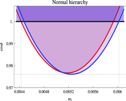
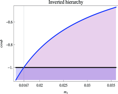
Figure 1: $\cos\varphi$ versus the lightest neutrino mass for the NO (left) and IO (right) cases. For the NO plot the most conservative limits are obtained for $\Delta m^{2}_{atm}=(2.46-0.15)\times 10^{-3}~{}{\rm eV}^{2}$ together with $\Delta m^{2}_{sol}=(7.67-0.21)\times 10^{-5}~{}{\rm eV}^{2}$ (left red curve), and with $\Delta m^{2}_{sol}=(7.67+0.22)\times 10^{-5}~{}{\rm eV}^{2}$ (right blue curve). For the IO plot the most conservative limit is obtained for $\Delta m^{2}_{atm}=(2.45-0.15)\times 10^{-3}~{}{\rm eV}^{2}$ and $\Delta m^{2}_{sol}=(7.67-0.21)\times 10^{-5}~{}{\rm eV}^{2}$.

For NO we have both a lower and an upper bound on $m_{1}$, that select a rather small range for the possible $m_{1}$ values of width $\sim\sqrt{3}\,r$ and centered around $m_{\rm sol}/\sqrt{3}$. Thus, the neutrino mass spectrum is essentially determined. From Fig. 1 we can also see that the phase $\varphi$ always remains quite close to zero ($\cos\varphi\ \hbox to0.0pt{\raise 3.0pt\hbox{$<$}\hss}{\lower 3.0pt\hbox{$\sim$}}\ \pi/15$), and that both the upper and lower bounds are saturated for $\varphi=0$. In the IO case, we only get a lower bound on $m_{3}$, that is saturated for $\varphi=\pm\pi$. The neutrino mass remains unbounded from above, and the phase $\varphi$ is allowed to vary between $\pi/2$ and $\pi$ or between $-\pi$ and $-\pi/2$, that is in the ranges where $\cos\varphi$ is negative.

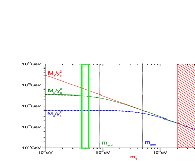
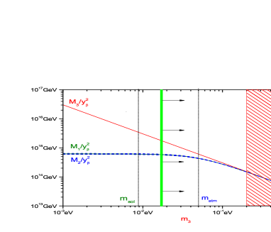
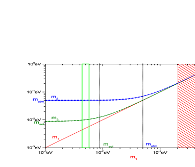
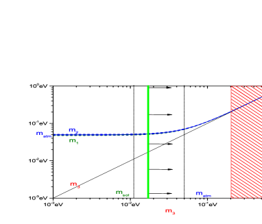
Figure 2: Plots of the heavy (upper panels) and light (lower panels) neutrino masses divided by $y_{\beta}^{2}$, as a function of the lightest left-handed neutrino mass, according to eq. (42). In the left panels (NO case) the two vertical green lines show the allowed $m_{1}$ mass range as given in eq. (50). In the right panels (IO case) the vertical green line shows the lower limit on $m_{3}$ eq. (51). The dashed area is the region excluded at $95\%\,{\rm CL}$ by the upper bound (cf. Eq. (57)) obtained by combining the cosmological upper bound on the sum of neutrino masses with neutrino oscillations data.

The results presented so far are of course approximate since the model gets corrections when higher dimensional operators are included in the Lagrangian. The inclusion of higher dimensional operators has also the effect of shifting the VEVs of the flavon fields from their leading order values, eq. (33). By assuming that the VEVs of the flavon fields have similar values $v_{T}\approx v_{S}\approx u\approx V$, these corrections modify the leading order approximation by terms of relative order $V/\Lambda$. The allowed range of $V/\Lambda$ is determined by the requirement that sub-leading corrections which perturb the leading order result are not too large and by the requirement that the $\tau$ Yukawa coupling $y_{\tau}$ does not become too large. The first requirement results in an upper bound on $V/\Lambda$ of about $0.05$, which mainly comes from the fact that the solar mixing angle should remain in its $1\sigma$ range. The second one gives a lower bound which we estimate as

$$\frac{V}{\Lambda}\approx\displaystyle\frac{\tan\beta}{y_{\tau}}\displaystyle\frac{m_{\tau}}{v}\approx 0.01\displaystyle\frac{\tan\beta}{y_{\tau}}~{}~{}~{}.$$ (54)

By asking $|y_{\tau}|<3$ we find a lower limit on $V/\Lambda$ close to the upper bound $0.05$ for $\tan\beta=15$, whereas $\tan\beta=2$ gives as lower limit $V/\Lambda>0.007$. We choose as maximal range:

$$0.007<\displaystyle\frac{V}{\Lambda}<0.05~{}~{}~{},$$ (55)

which shrinks when $\tan\beta$ is increased from 2 to 15.

In particular the leading order expressions of neutrino masses are modified by terms of relative order $V/\Lambda$. However, close to $\cos\varphi=\pm 1$, where the bounds are saturated, the corrections to both the numerator and the denominator of eq. (49) remain of relative order $V/\Lambda$, and thus the bounds in eq. (50) and eq. (51) are not significantly affected. For normal hierarchy, that requires $\cos\varphi$ very close to one in the full allowed mass range of eq. (50), the leading expression for $\cos\varphi$ given in eq. (49) always remains a good approximation. In the case of inverted hierarchy, close to $\cos\varphi=-1$, when $m_{3}$ is near its lower bound, the corrections are also negligible. Deviations from eq. (49) can become significant when $\cos\varphi$ approaches $-0.2$. This happens for $m_{3}\approx 0.09$ eV and $m_{1,2}\approx 0.10$ eV, that is when the spectrum becomes nearly degenerate.

It is interesting to estimate the order of magnitude for the RH neutrinos masses. Since no suppression is expected for parameters that are unrelated to the breaking of the flavor symmetry, we take $y_{\beta}={\cal O}(1)$. With this, and using as the light mass scale in the seesaw equation (42) $m_{\rm atm}\simeq 0.05\mathrm{eV}$, we obtain

$$M_{i}\sim 10^{14\div 15}\mathrm{GeV}\,.$$ (56)

A detailed summary of the neutrino mass relations and bounds is given in figure 2, where we have plotted the three light and the three heavy neutrino masses, taking into account both the information from neutrino oscillations data (cf. eq. (3.3)) and the seesaw relations eq. (42). In this way, at leading order, all six masses can be expressed as a function of just one independent parameter, that can be conveniently chosen to be the lightest left-handed neutrino mass $m_{l}$. Of course there is also a dependence on the neutrino mass ordering, namely if $m_{l}=m_{1}$ or $m_{l}=m_{3}$. In the figures we also display the cosmological upper bound on $m_{l}$

$$m_{l}<0.2\,{\rm eV}\;\;(95\%\,{\rm CL})\,,$$ (57)

that follows from the WMAP5 [30] upper bound on the sum of the three neutrino masses combined with the constraints from mass squared differences from oscillations data (cf. eq. (3.3)).

3.4 Neutrinoless double-$\beta$ decay

In the approximation of neglecting terms of higher order in the symmetry breaking, as well as RGE running effects from the high scale to the eV scale, we can straightforwardly obtain predictions for the $0\nu 2\beta$ decay parameter $|m_{ee}|$ for both the NO and IO cases. The $0\nu 2\beta$ decay parameter is defined as

$$|m_{ee}|=\left|\sum_{i}(U_{\nu})_{ei}^{2}m_{i}\right|\,,$$ (58)

and corresponds to the (11) entry in the neutrino mass matrix $m_{\nu}$ in eq. (41):

$$|m_{ee}|=|(m_{\nu})_{11}|=v_{u}^{2}\,y^{2}\,\left|\frac{2}{3(a+b)}+\frac{1}{3a}\right|\,.$$ (59)

In terms of physical neutrino masses, and to the order we are working here ($(U_{\nu})_{13}=0$) eq. (58) assumes the particularly simple form:

$$|m_{ee}|=\left|\frac{2}{3}m_{1}e^{i\alpha_{1}}+\frac{1}{3}m_{2}e^{i\alpha_{2}}\right|\,,$$ (60)

and thus depends only the phase difference $\alpha_{2}-\alpha_{1}$, where $\alpha_{i}$ are the phases of the diagonal matrix $U_{PH}$ defined below eq. (40).

In order to compute the allowed range of $|m_{ee}|$ when the lightest neutrino mass is allowed to vary in the allowed region eq. (50) (for NO) or eq. (51) (for IO), it is more convenient to express $|m_{ee}|$ directly in terms of the phase $\cos\phi$ in eq. (49). This can be done more easily by using eq. (59), and yields:

$$|m_{ee}|=\frac{m_{2}}{3}\sqrt{1+4\>\frac{2+|z|\cos\phi}{1+|z|^{2}+2|z|\cos\phi}}\,,$$ (61)

that holds for both NO and IO.

Following [31] we parameterize the forecast sensitivity of future $0\nu 2\beta$ experiments as

$$|m_{ee}|\to 10\,h\>{\rm meV},$$ (62)

where $h=0.6\div 2.8$ parameterizes the theoretical uncertainty related to different nuclear matrix elements calculations. We then confront the prediction of the $A_{4}\times Z_{3}\times U(1)_{FN}$ model with eq. (62).

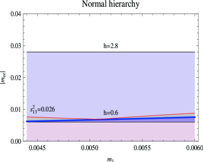
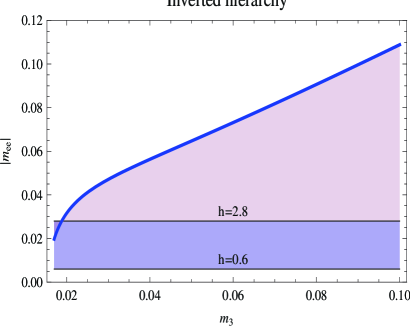
Figure 3: $|m_{ee}|$ versus the lightest neutrino mass. Left panel: the NO case. The thick blue line depict the value of $|m_{ee}|$ as a function of $m_{1}$. The thin red line illustrates the size of the corrections that could arise for $\sin^{2}\theta_{13}\approx 0.026$. Right panel: $|m_{ee}|$ as a function of $m_{3}$ in the IO case. In both cases the dark shaded horizontal region depicts the projected sensitivity of future $0\nu 2\beta$ experiments.

For the NO case we have $m_{l}=m_{1}$ and, according to eq. (50), $m_{l}$ can vary between $0.0044\,$eV and $0.0060\,$eV. The results for $|m_{ee}|$ in this case are depicted with the thick blue line in the left panel of figure 3. The dark horizontal region corresponds to the expected sensitivity of future $0\nu 2\beta$ experiments according to eq. (62). In the leading order approximation only $m_{1}$ and $m_{2}$ contribute to $|m_{ee}|$ (see eq. (60)). In the NO case these are the two smaller masses, and it is then reasonable to ask to what extent effects related to the largest mass $m_{3}$, that also contributes to $|m_{ee}|$ when $\sin^{2}\theta_{13}\neq 0$, can affect these results. By inserting in $U_{\nu}$ the maximum value $\sin^{2}\theta_{13}\approx 0.026$ allowed at 1$\sigma$ by present data [27], with the value of $m_{3}$ fixed in terms of $m_{1}$ and the mass squared differences, we obtain the values of $|m_{ee}|$ depicted in figure 3 (left panel) with the thin red line. Of course, the procedure of setting $(U_{\nu})_{13}\neq 0$ by hand, and not as a result of the inclusion of higher order terms, can just give a feeling of the possible effects of a non-vanishing $\sin^{2}\theta_{13}$, but does not correspond in any way to an improved prediction, that would require a consistent treatment of all higher order effects.

From the left panel in figure 3 we can then conclude that for all the allowed values of $m_{l}$, even in the most optimistic situation, $|m_{ee}|$ remains at best marginally in the reach of the future experiments sensitivity. We also see that higher order contributions $\propto m_{3}\cdot\sin^{2}\theta_{13}$ are not expected to change this conclusion.

For the IO we have $m_{l}=m_{3}$. A plot of $|m_{ee}|$ as a function of $m_{3}>0.017\,$eV (see eq. (51)) is depicted with a thick blue line in the right panel of figure 3. We see that in the IO case, $|m_{ee}|$ remains well above the sensitivity of future experiments, except in the most pessimistic situation ($h=2.8$) and when the lower bound is saturated ($m_{3}\sim 0.017\,$eV). In this situation the interference of the two contributions in eq. (60) is maximally destructive, yielding $|m_{ee}|\simeq m_{\rm atm}/3$. The results plotted in figure 3 (right panel) will not be significatively affected by contributions $\propto m_{3}\cdot\sin^{2}\theta_{13}$, that for IO are surely negligible, or by other higher order effects. Thus, the $A_{4}\times Z_{3}\times U(1)_{FN}$ model predicts that if the neutrino ordering is inverted, a $0\nu 2\beta$ decay signal quite likely will be observed in the next future. Detection of $0\nu 2\beta$ decay is guaranteed if new theoretical computations will establish that $h\ \hbox to0.0pt{\raise 3.0pt\hbox{$<$}\hss}{\lower 3.0pt\hbox{$\sim$}}\ 1.7$.

4 Leptogenesis in the $A_{4}\times Z_{3}\times U(1)_{FN}$ model

In section 2.2.1 we have shown that an important consequence of non-Abelian flavor symmetries with the $N_{i}$ assigned to an irreducible representation of the symmetry group, is that the leptogenesis CP asymmetries vanish at leading order. Their size is thus determined by the size of the flavor symmetry breaking parameters $\eta$. In the $A_{4}\times Z_{3}\times U(1)_{FN}$ the heavy Majorana masses are bounded from below by $M_{i}/y_{\beta}^{2}\ \hbox to0.0pt{\raise 3.0pt\hbox{$>$}\hss}{\lower 3.0pt\hbox{$\sim$}}\ 1.5\times 10^{14}\,$GeV (see upper right panel in figure 2), and thus are generally quite large. Therefore, the condition $M_{i}\gtrsim 10^{12}\,(1+\tan^{2}\beta)\,$GeV, that ensures that leptogenesis occurs in the unflavored regime, is generally matched by all the $N_{i}$ for natural values of the parameters (e.g. $\tan\beta\ \hbox to0.0pt{\raise 3.0pt\hbox{$<$}\hss}{\lower 3.0pt\hbox{$\sim$}}\ 10$ and $y\ \hbox to0.0pt{\raise 3.0pt\hbox{$>$}\hss}{\lower 3.0pt\hbox{$\sim$}}\ 0.5$ (NO) or $y\ \hbox to0.0pt{\raise 3.0pt\hbox{$>$}\hss}{\lower 3.0pt\hbox{$\sim$}}\ 0.8$ (IO)). In this regime, the relevant quantities that have to be considered are the total CP asymmetries $\varepsilon_{i}$, and since these asymmetries are ${\cal O}(\eta^{2})$ (see eq. (15)), the requirement of successful leptogenesis can provide hints on the minimum size of the typical symmetry breaking effects. The important point here is that in general the symmetry breaking parameters are also related to some observables that are measurable at low energy. For example, in models that predict neutrinos tribimaximal mixing (TBM) (as is the case of our $A_{4}\times Z_{3}\times U(1)_{FN}$ model) both the value of $\theta_{13}$ and the deviation from maximal angle of $\theta_{23}$ are related to $\eta$ and, by studying leptogenesis, one can infer preferred ranges of values for these parameters. This is a new type of low-energy/high-energy connection (see however [8, 32]) and constitutes the main motivation of the following analysis.

4.1 The leptogenesis CP asymmetries at subleading order

Since in our $A_{4}$ model the heavy Majorana neutrinos belong to an irreducible representation of the flavor group, independently of the particular basis we have that ${\cal Y}^{0}\equiv{Y}^{0\dagger}{Y^{0}}=y^{2}\,\mathbb{I}$. Thus, at leading order, all the CP asymmetries vanish. When the leading symmetry breaking terms are introduced in the Lagrangian, new complex parameters are generated that give rise to non-vanishing CP asymmetries (see eqs. (14) and (15)).

All the possible leading order corrections to the $A_{4}\times Z_{3}\times U(1)_{FN}$ model have been listed in [6]. However, as long as the CP asymmetry are concerned, the relevant terms are only two [8], and both represent corrections to the Majorana neutrinos Yukawa matrix:

$$\frac{y_{1}}{\Lambda}\left(\varphi_{T}\left(\ell N\right)_{S}\right)H_{u},\qquad\qquad\displaystyle\frac{y_{2}}{\Lambda}\left(\varphi_{T}\left(\ell N\right)_{A}\right)H_{u}\,.$$ (63)

Using the product rules of eqs. (28-30), the Yukawa matrix now reads:

$$Y=Y^{0}+\delta Y=\left(\begin{array}[]{ccc}y+2d&0&0\\ 0&0&y-d+c\\ 0&y-d-c&0\\ \end{array}\right)$$ (64)

where we have introduced the two complex numbers $c,d$ ($|c|,|d|\ll y$) defined as

$$c\equiv\frac{y_{2}v_{T}}{2\Lambda},\qquad\qquad d\equiv\frac{y_{1}v_{T}}{3\Lambda}\,.$$ (65)

Assuming, as is reasonable to do, that $y_{1}$ and $y_{2}$ are numbers of the same order, we can parameterize the size of the symmetry breaking effects with a single hierarchical parameter $\eta$, defining for example

$$\eta={\rm Re}(d)\hskip 28.45274pt\mbox{\rm and}\hskip 28.45274pt\rho={{\rm Re}(c)\over{\rm Re}(d)}\,,$$ (66)

where $\rho={\cal O}(1)$. Then in the hatted basis the matrix $\hat{\cal Y}={\hat{Y}}^{\dagger}{\hat{Y}}$ becomes

$$\begin{array}[]{lll}\hat{\cal Y}&=&U_{PH}^{-1}U_{TB}^{T}{\cal Y}~{}U_{TB}U_{PH}\\ &&\\ &=&y\cdot\left(\begin{array}[]{ccc}y+2\,\eta&2\sqrt{2}\,\eta\,e^{i\alpha_{21}}&-\displaystyle\frac{2}{\sqrt{3}}\,\rho\,\eta\,e^{i\alpha_{31}}\\ 2\sqrt{2}\,\eta\,e^{i\alpha_{12}}&y&2\sqrt{\displaystyle\frac{2}{3}}\,\rho\,\eta\,e^{i\alpha_{32}}\\ -\displaystyle\frac{2}{\sqrt{3}}\,\rho\,\eta\,e^{i\alpha_{13}}&2\sqrt{\frac{2}{3}}\,\rho\,\eta\,e^{i\alpha_{23}}&y-2\,\eta\\ \end{array}\right)\,.\end{array}$$ (67)

Since $\hat{\cal Y}$ is a physical observable (it can be measured in principle by measuring the CP asymmetries) it depends only on phase differences $\alpha_{ij}\equiv(\alpha_{i}-\alpha_{j})/2$.

Recalling now the expressions of the CP asymmetries given in eq. (6) in terms of $\hat{\cal Y}$ and of the functions $f_{ij}$ (see eq. (8)) we can write:

$$\varepsilon_{1} = \frac{\eta^{2}}{8\pi}\left(8\,\sin\left(2\alpha_{21}\right)f_{12}+\frac{4}{3}\,\rho^{2}\,\sin\left(2\alpha_{31}\right)f_{13}\right)$$

$$\varepsilon_{2} = \frac{\eta^{2}}{8\pi}\left(-8\,\sin\left(2\alpha_{21}\right)f_{21}+\frac{8}{3}\,\rho^{2}\,\sin\left(2\alpha_{32}\right)f_{23}\right)$$

$$\varepsilon_{3} = \frac{\eta^{2}}{8\pi}\left(-\frac{4}{3}\,\rho^{2}\,\sin\left(2\alpha_{31}\right)f_{31}-\frac{8}{3}\,\rho^{2}\,\sin\left(2\alpha_{32}\right)f_{32}\right)\,.$$ (68)

Starting from $2\,\alpha_{21}=-\mathrm{arg}(a)+\mathrm{arg}(a+b)$ and $2\,\alpha_{32}=\mathrm{arg}(a)-\mathrm{arg}(-a+b)$, one finds the following relations

$$\sin(2\,\alpha_{21}) = {|z|\,\sin\varphi\over\sqrt{1+2\,|z|\,\cos\varphi+|z|^{2}}}\,,$$

$$\sin(2\,\alpha_{32}) = -{|z|\,\sin\varphi\over\sqrt{1-2\,|z|\,\cos\varphi+|z|^{2}}}\,,$$

$$\sin(2\,\alpha_{31}) = -{2\,|z|\,\sin\varphi\over\sqrt{(|z|^{2}-1)^{2}+4\,|z|^{2}\,\sin^{2}\varphi}}\,.$$ (69)

We recall that, after expressing the heavier neutrino masses in terms of $m_{\rm sol}$, $m_{\rm atm}$ and $m_{l}$, one has that $\sin(2\alpha_{21})$, $\sin(2\alpha_{32})$ and $\sin(2\alpha_{31})$ in eq. (4.1) are a function of $m_{l}$ only. Moreover, given that the expressions for the $\varepsilon_{i}$ depend, through the functions $f_{ij}$, only on ratios of the heavy Majorana masses $M_{i}$, and that through the seesaw formula eq. (41) these ratios are directly related to the ratios of light neutrino masses $m_{i}$, we can conclude that the CP-asymmetries in eq. (4.1) depend only on $m_{l}$, on the non-hierarchical parameter $\rho$, and on the parameter $\eta$ that quantifies the flavor symmetry breaking effects.

4.2 Analytic approximations

In this Section we present simple analytical formulae to estimate the matter-antimatter asymmetry produced via leptogenesis within the $A_{4}\times Z_{3}\times U(1)_{FN}$ model. The presence of the heaviest RH neutrino makes possible for the $C\!P$ asymmetry $\varepsilon_{2}$ of the next-to-lightest RH neutrino to be unsuppressed (cf. (4.1)) compared to the $C\!P$ asymmetry of the lightest RH neutrino, even when the RH neutrino spectrum is strongly hierarchical [33]. Furthermore, since in our case the heavy neutrino spectrum is only mildly hierarchical, even the $C\!P$ asymmetry of the heaviest RH neutrino is not particularly suppressed. Therefore, all the three contributions to the final asymmetry have to be taken into account since in the presence of compensating effects from reduced wash-outs the $B-L$ asymmetry generated in the decays of the heaviest RH neutrinos could become comparable to the one generated in the decays of the two lighter RH neutrinos. This situation is indeed realized in the NO case.

For our estimates, we adopt the following simplifications:

• For the reasons explained in the beginning of the Section, we assume that leptogenesis occurs in the unflavored regime.

• The $A_{4}\times Z_{3}\times U(1)_{FN}$ model must be supersymmetric, since the vacuum alignment conditions eq. (33) are fulfilled within a supersymmetric framework [6]. Our results are instead obtained neglecting all supersymmetric partners effects. This underestimates the resulting $B-L$ asymmetry by a factor $\approx\sqrt{2}$ (see ref. [34] and [15] Sec. 10).

• The value of the final $B-L$ asymmetry that we estimate is obtained by summing up the asymmetries generated in the decays of the three heavy neutrinos [11, 37] but neglecting the wash-out of the asymmetry due to the inverse processes of the lighter RH neutrinos [35, 36]. This can be done because, neglecting ${\cal O}(\eta^{2})$ terms, the leptons produced in the decays of the three RH neutrinos are orthogonal to each other:

  $$|\langle L_{i}|L_{j}\rangle|^{2}=\frac{|\hat{\cal Y}_{ji}|^{2}}{|\hat{\cal Y}_{jj}\hat{\cal Y}_{ii}|}=\delta_{ij}+{\cal O}(\eta^{2})\,.$$ (70)

  Doing this we are slightly overestimating the final asymmetry since we neglect the fact that the three lepton states $|L_{i}\rangle=(\hat{\cal Y}_{ii})^{-1/2}\,\sum_{\alpha}\hat{Y}^{*}_{\alpha i}|L_{\alpha}\rangle$ produced in $N_{i}$ decays are not exactly orthogonal one to the other, and thus part of the asymmetry produced by the heavier states gets washed out by the lighter RH neutrinos interactions. These effects could be taken into account in a straightforward way following the procedure explained in in [35]. However, neglecting the wash-out from lighter RH neutrinos is certainly consistent with the order of our approximation since, e.g. relative ${\cal O}(\eta)$ corrections to the CP asymmetries, that could produce even larger effects, are also neglected. With this approximation we also do not have to worry about complications coming from an overlap between decays and inverse decays that occur when the RH neutrino mass spectrum is not strongly hierarchical, and the leptons produced in the decays of the three RH neutrinos are not orthogonal to each other [38].

• We neglect subleading leptogenesis effects like $\Delta L=1$ scatterings [39, 40, 4, 41] and CP violation in scatterings [42], thermal corrections [4], spectator processes [43, 44], departure from kinetic equilibrium [45]. In the strong wash-out regime that is the relevant one for our model, these effects give corrections at most at the level of $\sim 50\%$.

With these approximations, the $B-L$ asymmetry can be estimated by solving the following three independent pairs of Boltzmann equations

$${dN_{N_{i}}\over dz_{i}} = -D_{i}\,(N_{N_{i}}-N_{N_{i}}^{\rm eq})\;,\hskip 28.45274pt(i=1,2,3)$$ (71)

$${dN^{(i)}_{B-L}\over dz_{i}} = \varepsilon_{i}\,D_{i}\,(N_{N_{i}}-N_{N_{i}}^{\rm eq})-N_{B-L}^{(i)}\,[W_{i}(z_{i})+\Delta W_{i}(z_{i})]\,,$$ (72)

where $z_{i}\equiv M_{i}/T$. We indicated with $N_{X}$ any particle number or asymmetry $X$ calculated in a portion of co-moving volume containing one heavy neutrino in ultra-relativistic thermal equilibrium, so that $N^{\rm eq}_{N_{i}}(T\gg M_{i})=1$. With this convention the predicted baryon-to-photon ratio $\eta_{B}$ is related to the final value of the $B-L$ asymmetry $N_{B-L}$ by the relation

$$\eta_{B}=a_{\rm sph}{N_{B-L}^{\rm f}\over N_{\gamma}^{\rm rec}}\simeq 0.96\times 10^{-2}\,N_{B-L}\,,$$ (73)

where $N_{\gamma}^{\rm rec}\simeq 37$, and $a_{\rm sph}=28/79$. The decay factors are given by

$$D_{i}\equiv{\Gamma_{{\rm D},i}\over H\,z_{i}}=K_{i}\,z_{i}\,\left\langle{1\over\gamma_{i}}\right\rangle\,.$$ (74)

Moreover, indicating with $g_{\star}=g_{SM}=106.75$ the total number of degrees of freedom and with $M_{\rm Pl}=1.22\,\times\,10^{19}\,{\rm GeV}$ the Planck mass, the expansion rate can be expressed as

$$H(z_{i})=\sqrt{8\,\pi^{3}\,g_{\star}\over 90}{M_{i}^{2}\over M_{\rm Pl}}\,{1\over z_{i}^{2}}\simeq 1.66\,\sqrt{g_{\star}}\,{M_{i}^{2}\over M_{\rm Pl}}\,{1\over z_{i}^{2}}\,.$$ (75)

The total decay rates, $\Gamma_{{\rm D},i}=(\Gamma_{i}+\bar{\Gamma}_{i})\,\langle 1/\gamma_{i}\rangle$, are the product of the decay widths times the thermally averaged dilation factors that can be expressed in terms of the ratio of the modified Bessel functions, such that $\langle 1/\gamma_{i}\rangle={\cal K}_{1}(z_{i})/{\cal K}_{2}(z_{i})$ . The equilibrium abundance and its rate can be also expressed in terms of the modified Bessel functions:

$$N_{N_{i}}^{\rm eq}(z_{i})={1\over 2}\,z_{i}^{2}\,{\cal K}_{2}(z_{i})\;\;,\hskip 28.45274pt{dN_{N_{i}}^{\rm eq}\over dz_{i}}=-{1\over 2}\,z_{i}^{2}\,{\cal K}_{i}(z_{i})\,.$$ (76)

Introducing the effective washout parameters [40]

$$\widetilde{m}_{i}=v^{2}\frac{\mathcal{Y}_{ii}}{M_{i}}$$ (77)

and the equilibrium neutrino mass [46, 3]

$$m_{\star}=\frac{16\pi^{5/2}\sqrt{g_{\star}}}{3\sqrt{5}}\frac{v^{2}}{M_{Pl}}\simeq 1.08\times 10^{-3}~{}\mathrm{eV}\,,$$ (78)

the decay parameters can be expressed as

$$K_{i}\equiv{\Gamma_{i}+\bar{\Gamma}_{i}\over H(z_{i}=1)}={\widetilde{m}_{i}\over m_{*}}\,.$$ (79)

In our case, from the Eq. (67) one can verify that $\widetilde{m}_{i}\simeq m_{i}$ and therefore there is a very simple relation between neutrino masses and decay parameters.

After proper subtraction of the resonant contribution from $\Delta L=2$ processes [47], the inverse decay washout terms are given by

$$W_{i}(z_{i})={1\over 4}\,K_{i}\,{\cal K}_{1}(z_{i})\,z_{i}^{3}\,.$$ (80)

The wash-out term $\Delta W_{i}(z_{i})$ is the non-resonant contribution to the wash-out coming from $\Delta L=2$ processes and can be written as

$$\Delta W_{i}(z_{i})\simeq{\alpha\over z_{i}^{2}}\,M_{i}\,\widetilde{m}_{i}^{2}\,,$$ (81)

where

$$\alpha={3\,\sqrt{5}\,M_{\rm Pl}\over 4\,\zeta(3)\,\pi^{9/2}\,v^{4}\,\sqrt{g_{\star}}}\,.$$ (82)

The $B-L$ asymmetry produced from $N_{i}$-decays can then be estimated as [5]

$$N^{(i)}_{B-L}=\,\varepsilon_{i}\,\kappa(K_{i})\,e^{-{\alpha\over z_{B}(K_{i})}\,M_{i}\,\widetilde{m}_{i}^{2}},$$ (83)

where $\kappa(K_{i})$ accounts for the wash-out from inverse processes and is approximately given by

$$\kappa(K_{i})={2\over K_{i}\,z_{B}(K_{i})}\,\left(1-e^{-{K_{i}\,z_{B}(K_{i})\over 2}}\right)\,.$$ (84)

The quantity

$$z_{B}(K_{i})\simeq 2+4\,{K_{i}}^{0.13}\,e^{-{2.5\over K_{i}}}$$ (85)

gives the approximate the value of $z_{i}$ around which the final asymmetry from $N_{i}$-decays is dominantly produced.

The exponential factor in eq. (83) accounts for the wash-out from $\Delta L=2$ processes. One can notice that the two wash-out contributions factorize. Notice also that the $\Delta L=2$ processes suppression is relevant only for $M_{i}\gtrsim 10^{14}\,{\rm GeV}\,(0.05\,{\rm eV}/m_{i})^{2}$.

Finally, using eq. (83) and eq. (73), the baryon to photon number ratio can be written as

$$\eta_{B}=\sum_{i}\eta_{i}\simeq 0.96\times 10^{-2}\ \sum_{i}\,\varepsilon_{i}\,\kappa(K_{i})\,\,e^{-{\alpha\over z_{B}(K_{i})}\,M_{i}\,m_{i}^{2}}.$$ (86)

This theoretical prediction has to be compared with the observed value from WMAP data [30]

$$\eta_{B}^{\rm CMB}=(6.2\pm 0.15)\times 10^{-10}\,.$$ (87)

4.3 Results

We now describe the results for $\eta_{B}$, separating the discussion for the NO and the IO case.

4.3.1 Normal Ordering

In the upper panels of Fig. 4 we show the dependence on $m_{1}=m_{l}$ of the three CP asymmetries $\varepsilon_{i}$ divided by the square of symmetry breaking parameter $\eta^{2}$ for positive values of $\sin\varphi$. For negative values they are simply all opposite. Therefore, by switching the sign of $\sin\varphi$ the sign of the final baryon asymmetry changes as well (i.e., the model does not predict the sign of the baryon asymmetry). It turns out that the correct sign of the baryon asymmetry is obtained for $\sin\varphi<0$. In the lower panels of Fig. 4 we show the absolute values of $\eta_{i}/\eta^{2}$ ($i=1,2,3$), that is the relevant quantity, together with the total value $|\eta_{B}|=|\sum_{i}\eta_{i}|$.

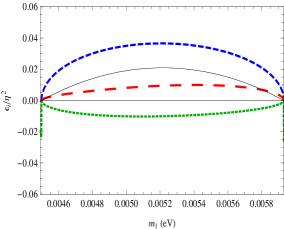
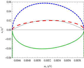
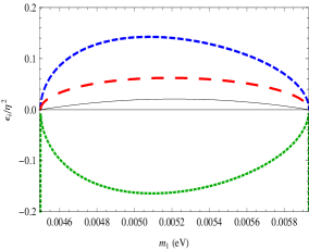
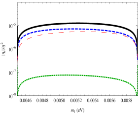
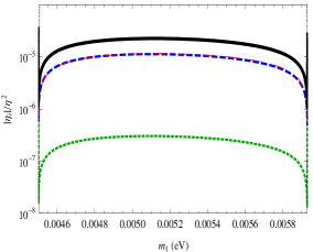
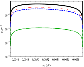
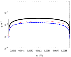
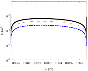
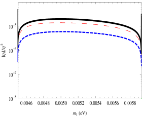
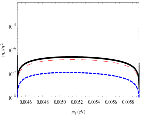
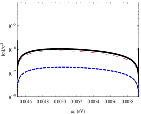
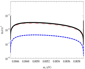
Figure 4: NO. In the 3 upper panels we plot the CP asymmetries $\varepsilon_{i}$ divided by $\eta^{2}$ as a function of $m_{1}$ for $\sin\varphi>0$ (note the different vertical scale in the last panel). The dashed line corresponds to $i=1$, the short-dashed line to $i=2$ and the dotted line to $i=3$. The solid line is $1-\cos\varphi$ (cf. Eq. (49)). In the 9 lower panels we have plotted the three $|\eta_{i}|/\eta^{2}$ (cf. Eq. (86)), with the same line convention as for the $C\!P$ asymmetries for $i=1,2,3$ respectively, and $|\eta_{B}|/\eta^{2}$ (solid line). All the left panels correspond to $\rho=0.5$, all the central panels to $\rho=1$ and all the right panels to $\rho=2$. The three rows of nine lower panels, showing the asymmetries, correspond to $y_{\beta}=1$, $y_{\beta}=2$ and $y_{\beta}=3$ starting from above.

We show the plots for three different values of $\rho=0.5,1,2$ from left to right and for three different values of $y_{\beta}=1,2,3$ from above to below. One can see how for increasing $\rho$ typically the finally asymmetry increases.

On the other hand, increasing $y_{\beta}$, the three RH neutrino masses increase up to a critical value above which there is an exponential suppression from $\Delta L=2$ processes. This critical value is about $y_{\beta}\sim 2$ and for $y_{\beta}=3$ the value of $\eta_{B}/\eta^{2}$ reproduces the observed asymmetry for the highest possible values of the $\eta$-range $5\times 10^{-3}\div 5\times 10^{-2}$.

It is also interesting to notice that the contribution from the lightest RH neutrinos (depicted in Fig. 4 with the green dotted line) is sub-dominant, despite the fact that the lightest RH neutrino $C\!P$ asymmetry $|\varepsilon_{3}|$ is typically the highest or anyway comparable to $|\varepsilon_{2}|$ (depending on the value of $m_{1}$). The reason is that $K_{3}\simeq m_{\rm atm}/m_{\star}\gg K_{1,2}$ and therefore the wash-out is much stronger compared to the two heavier RH neutrinos.

In Fig. 5 we have plotted, as a function of $m_{1}$ and for different choices of $\rho$ and $y_{\beta}$, the value of $\eta$ such that $\eta_{B}=\eta_{B}^{CMB}$. One can see that this value always falls in the optimal range $\eta=5\times 10^{-3}\div 5\times 10^{-2}$ (the grey band).

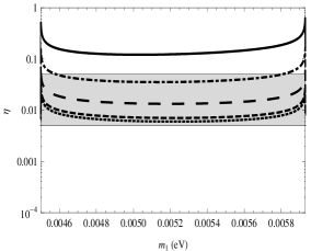
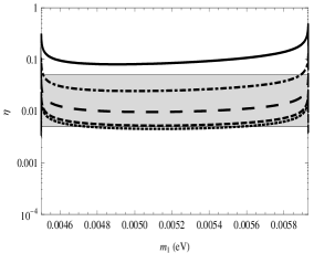
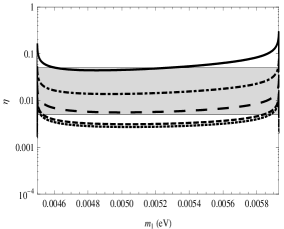
Figure 5: NO. Plots of the values of $\eta$ that reproduce the observed $\eta_{B}$, as a function of $m_{1}$ for $\rho=0.5$ (left panel), $\rho=1$ (central panel), $\rho=2$ (right panel). The different curves correspond to $y_{\beta}=0.5$ (dotted), $y_{\beta}=1$ (short-dashed), $y_{\beta}=2$ (long-dashed), $y_{\beta}=3$ (dot-dashed) and $y_{\beta}=4$ (solid). The gray band is the indicative optimal range of values of $\eta=5\times 10^{-3}\div 5\times 10^{-2}$.

It seems therefore that, despite the many constraints on the model parameters and in particular the fact that there is only one independent complex phase and that the single dimensional parameter $m_{1}$ is practically fixed, the model reproduces the observed baryon asymmetry for natural values of the parameters in quite a satisfactory way.

4.3.2 Inverted Ordering

In the upper panels of Fig. 6 we show the dependence on $m_{3}=m_{l}$ of the three $\varepsilon_{i}/\eta^{2}$ for positive values of $\sin\varphi$. Again, by switching the sign of $\sin\varphi$, one can always change the final sign of the final asymmetry and again the correct (positive) sign is obtained for $\sin\varphi<0$.

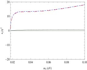
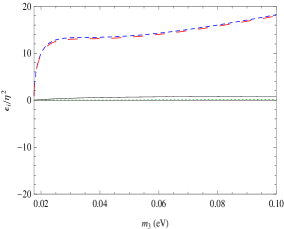
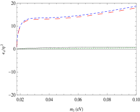
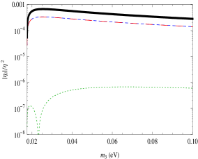
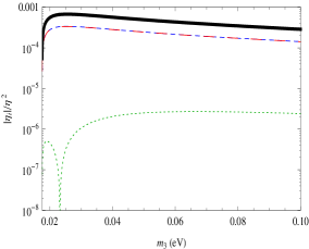
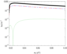
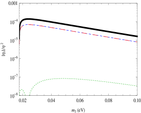
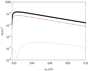
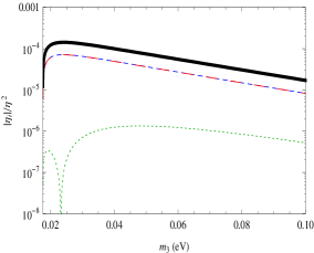
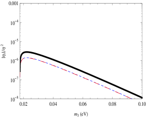
Figure 6: IO. In the 3 upper panels we plot the three $\varepsilon_{i}/\eta^{2}$ as a function of $m_{1}$ and for $\sin\varphi>0$. The dashed line corresponds to $i=1$, the short-dashed line to $i=2$ and the dotted line to $i=3$. The solid line is $1+\cos\varphi$ (cf. Eq. (49)). In the 9 lower panels we have plotted the three $|\eta_{i}|/\eta^{2}$ (cf. Eq. (86)) with the same line correspondence as for the $C\!P$ asymmetries and $|\eta_{B}|/\eta^{2}$ (solid line). All the left panels correspond to $\rho=0.5$, all the central panels to $\rho=1$ and all the right panels to $\rho=2$. The three rows of nine lower panels showing the asymmetries correspond to $y_{\beta}=0.5$, $y_{\beta}=1$ and $y_{\beta}=1.7$ starting from above.

We show again three different values of $\rho=0.5,1,2$ from left to right. However, one can see that now there is only a tiny dependence on $\rho$. The reason can be easily understood inspecting the three Eq.’s (4.1). The strong degeneracy between the two lower RH neutrino masses, $M_{1}$ and $M_{2}$, implies $|\xi(x_{2}/x_{1})|,|\xi(x_{1}/x_{2})|\sim 10^{3}$ and therefore $|f_{12}|,|f_{21}|\gg 1$. In this way the term depending on $\rho$ gives a negligible contribution.

We again show examples for three different values of $y_{\beta}$. This time we choose $y_{\beta}=0.5,1,1.7$ from above to below. One can see how for $y_{\beta}=0.5$ one has $\eta_{B}/\eta^{2}\sim 10^{-4}\div 10^{-3}$ and therefore too small values of $\eta\lesssim 10^{-3}$ are required to explain the observed asymmetry. On the other hand for $y_{\beta}=1.7$ one has $\eta_{B}/\eta^{2}\sim 10^{-8}\div 10^{-6}$ and this time too large values of $\eta\lesssim 5\times 10^{-2}\div 5\times 10^{-1}$ are needed. Therefore, in these examples, the observed asymmetry is reproduced for reasonable values of $\eta\sim 0.01$ only for $y_{\beta}=1$. For this value there is indeed a compensation between very large values of the $C\!P$ asymmetries, $|\varepsilon_{i}|\sim 10^{-2}$ for $\eta\sim 10^{-2}$, and an additional wash-out suppression $\sim 10^{-4}$ coming from $\Delta L=2$ processes so that the resulting efficiency factor $\sim 10^{-6}$.

We have again summarized the situation plotting in Fig. 7, the value of $\eta$ such that $|\eta_{B}|=\eta_{B}^{CMB}$ as a function of $m_{l}$. We show five examples for $y_{\beta}=0.5,1,1.3,1.7,2$. One can see that this time $\eta$ naturally falls in the optimal range $\eta=5\times 10^{-3}\div 5\times 10^{-2}$ (the grey band) only for for $y_{\beta}=1\div 1.7$, therefore requiring some amount of tuning.

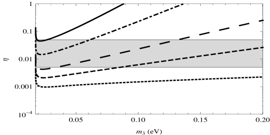
Figure 7: IO. Plot of the values of $\eta$ that reproduce the observed $\eta_{B}$, as a function of $m_{1}$ for $\rho=1$. The different curves correspond to $y_{\beta}=0.5$ (dotted), $y_{\beta}=1$ (dashed), $y_{\beta}=1.3$ (long-dashed), $y_{\beta}=1.7$ (dot-dashed) and $y_{\beta}=2$ (solid). The gray band is the indicative optimal range of values of $\eta=5\times 10^{-3}\div 5\times 10^{-2}$.

Moreover this occurs not for all values of $m_{l}$ and in particular values $y_{\beta}\simeq 1$ require $m_{l}\gtrsim 0.1\,{\rm eV}$. Therefore, an improvement of the upper bound on $m_{l}$ (cf. (57)) will enforce higher values of $y_{\beta}$ corresponding to higher values of the RH neutrino masses that in turn imply higher values of the initial temperature of the radiation dominated regime that, in an inflationary language, corresponds to the reheating temperature of the Universe.

4.4 Reheating temperature constraints

The model predicts a RH neutrino spectrum with a mild hierarchy and an overall scale of values of the RH neutrino masses that is quite large. For NO one has $M_{3}\sim 10^{15}\,{\rm GeV}\,y^{2}_{\beta}$, where $M_{3}$ is the mass of the lightest RH neutrino. For IO the scale can be about five times lower if one considers quasi-degenerate light neutrinos with masses $m_{i}\gtrsim 0.1\,{\rm eV}$, close to the current cosmological upper bound (cf. (57)).

Since RH neutrinos are produced by thermal processes, this in turn implies a lower bound on the reheating temperature given approximately by [5] $T_{\rm reh}\gtrsim M_{\rm 3}/[z_{B}(K_{\rm 3})-2]\simeq 10^{14}\,y^{2}_{\beta}\,{\rm GeV}$ in the case of NO and about five times lower for IO. Are such high values of the $T_{\rm reh}$ possible ? Since our model is supersymmetric, the well known upper bound $T_{\rm reh}\lesssim 10^{6\div 10}\,{\rm GeV}$ from the avoidance of the gravitino problem potentially applies [48]. It is clear that such low values cannot be obtained in the presented version of the model since, even taking the low value $y_{\beta}\sim 0.1$, one obtains $T_{\rm reh}\gtrsim 10^{12}\,{\rm GeV}$ for NO.

There are two possible kinds of ways out remaining within thermal leptogenesis. The first one would be to circumvent the gravitino problem and indeed a few solutions have been proposed [49]. The second kind would be to modify the model in such a way that the overall RH neutrino mass scale is lowered. It would not be difficult to envisage different schemes to this extent.

On the other hand, in the case of IO the second strategy cannot be invoked for the simple reason that large values of the RH neutrino masses $M_{l}\gtrsim 10^{14}\,{\rm GeV}$ are necessary in order to get a strong additional wash-out suppression from $\Delta L=2$ processes to compensate the very large values of the $C\!P$ asymmetries. In other words large reheating temperatures $T_{\rm reh}\gtrsim 5\times 10^{13}\,{\rm GeV}$ cannot be avoided in the case of IO.

5 Conclusions

A typical outcome of extensions of the standard model that attempt to explain the features of the lepton mass spectrum on the basis of flavor symmetries is that small quantities such as the charged lepton mass ratios, $\Delta m^{2}_{sol}/\Delta m^{2}_{atm}$, $\theta_{23}-\pi/4$ and $\theta_{13}$ are proportional to some power of small symmetry breaking parameters $\eta$. By keeping only the leading order power of $\eta$, in some cases the number of independent parameters becomes small and these models can be rather predictive, with characteristic relations among the observable quantities. Well known examples are relations between the neutrino oscillation parameters and the branching ratios of lepton flavor violating processes, such as $\mu\to e\gamma$, $\tau\to\mu\gamma$ and $\tau\to e\gamma$. It would be quite interesting to include in this kinships also the baryon asymmetry, which, in the context of leptogenesis, is naturally related to lepton masses and mixing angles.

With such scope in our mind, we have discussed the constraints on the leptogenesis $C\!P$ asymmetries in models possessing a flavor symmetry. We have derived general conditions for the vanishing of the $C\!P$ asymmetries in the limit of exact flavor symmetry. We have shown that, if the three RH neutrinos belong to an irreducible representation of the flavor symmetry group, then the total $C\!P$ asymmetries are zero in the limit of exact flavor symmetry. More precisely, for non-degenerate RH neutrino masses, the total $C\!P$ asymmetries $\epsilon_{i}$ are of order $\eta^{2}$ and the flavored ones $\epsilon_{i\to\alpha}$ are of order $\eta$. If the RH neutrinos are not in an irreducible representation of the flavor group, we have derived a necessary and sufficient condition for the vanishing of the total $C\!P$ asymmetry in the symmetric limit and we have discussed it in several particular cases. For instance, if the action of the symmetry on RH neutrinos is Abelian, then in most cases the $C\!P$ asymmetries are of order $\eta^{0}$ and we should invoke additional washout suppression to reproduce the observed baryon asymmetry.

One interesting example of vanishing leading-order $C\!P$ asymmetries is that of a model symmetric under $A_{4}\times Z_{3}\times U(1)_{FN}$, built to reproduce tri-bimaximal lepton mixing. In this model RH neutrinos are in a triplet of $A_{4}$ and $\epsilon_{i}=O(\eta^{2})$. The model is rather constrained. Once the parameters are fixed to match $\Delta m^{2}_{sol}$ and $\Delta m^{2}_{atm}$, there is only one relevant phase $\varphi$, which can be thought of as a function of the lightest neutrino mass $m_{l}$. The RH neutrino spectrum depends only on an additional, $O(1)$, parameter $y_{\beta}$. Both normal and inverted neutrino mass ordering can be reproduced. For normal ordering $m_{l}$ is essentially fixed in a small range around $0.005$ eV and the phase should be very small. For inverted hierarchy there is a lower bound on $m_{l}$ of approximately $0.017$ eV and there is much more freedom for the phase. Given this rather constrained framework it is not guaranteed that a successful leptogenesis can take place at all and we computed the washout effects and the resulting baryon asymmetry. The dynamics of the model is quite interesting since the RH neutrinos have similar masses and they all participate to generate the baryon asymmetry. At the same time, to a good approximation, the asymmetry produced in the decay of one RH neutrino is not washed-out by the other heavy neutrino inverse processes, since the interactions of the three RH neutrinos with the light leptons are almost orthogonal to each other. For normal hierarchy we find that the observed baryon asymmetry is reproduced for values of the symmetry breaking parameter $\eta$ in the range $0.005\div 0.05$, which nearly coincides with the natural expected range in this model. This prediction is rather stable with respect to variation of $y_{\beta}$. For inverted hierarchy we find solutions in the parameter space, but they are less stable. If $0.005<\eta<0.05$, there is only a rather limited range of allowed values for $y_{\beta}$. On the one hand, for small values of $y_{\beta}$ the baryon asymmetry is typically enhanced, compared to the normal ordering case and we cannot go below $y_{\beta}\simeq 1$, with a reheating temperature not lower than $5\times 10^{13}$ GeV. On the other hand, as soon as $y_{\beta}$ exceeds 2 the suppression from the washout becomes huge and the baryon asymmetry goes rapidly to zero.

It is interesting that though the IO case has a much wider parameter freedom compared to the NO case, it certainly appears less attractive from a cosmological point of view. Future improvements on the measurements of the absolute neutrino mass scale will allow to test our results.

Acknowledgments We warmly acknowledge Emiliano Molinaro and Serguey Petcov for pointing out a mistake in eq. (4.1) in the first version of the paper. PDB was supported by the Helmholtz Association of National Research Centres, under project VH-NG-006. The work of EN is supported in part by Colciencias under contract 1115-333-18739.

References

- [1] P. Minkowski, Phys. Lett. B 67 (1977) 421; T. Yanagida, in Workshop on Unified Theories, KEK report 79-18 (1979) p. 95; M. Gell-Mann, P. Ramond, R. Slansky, in Supergravity (North Holland, Amsterdam, 1979) eds. P. van Nieuwenhuizen, D. Freedman, p. 315; S.L. Glashow, in 1979 Cargese Summer Institute on Quarks and Leptons (Plenum Press, New York, 1980) p. 687; R. Barbieri, D. V. Nanopoulos, G. Morchio and F. Strocchi, Phys. Lett. B 90 (1980) 91; R. N. Mohapatra and G. Senjanovic, Phys. Rev. Lett. 44 (1980) 912.
- [2] M. Fukugita, T. Yanagida, Phys. Lett. B 174 (1986) 45.
- [3] W. Buchmuller, P. Di Bari and M. Plumacher, Nucl. Phys. B 665 (2003) 445 [arXiv:hep-ph/0302092]; W. Buchmuller, P. Di Bari and M. Plumacher, New J. Phys. 6 (2004) 105 [arXiv:hep-ph/0406014].
- [4] G. F. Giudice, A. Notari, M. Raidal, A. Riotto and A. Strumia, Nucl. Phys. B 685 (2004) 89 [arXiv:hep-ph/0310123].
- [5] W. Buchmuller, P. Di Bari and M. Plumacher, Annals Phys. 315 (2005) 305 [arXiv:hep-ph/0401240].
- [6] G. Altarelli and F. Feruglio, Nucl. Phys. B 720, 64 (2005) [arXiv:hep-ph/0504165]; G. Altarelli and F. Feruglio, Nucl. Phys. B 741, 215 (2006) [arXiv:hep-ph/0512103]; G. Altarelli, F. Feruglio and Y. Lin, Nucl. Phys. B 775, 31 (2007) [arXiv:hep-ph/0610165]; G. Altarelli, F. Feruglio and C. Hagedorn, JHEP 0803 (2008) 052 [arXiv:0802.0090 [hep-ph]].
- [7] P. F. Harrison, D. H. Perkins and W. G. Scott, Phys. Lett. B 530, 167 (2002) [arXiv:hep-ph/0202074].
- [8] E. E. Jenkins and A. V. Manohar, Phys. Lett. B 668, 210 (2008) [arXiv:0807.4176 [hep-ph]].
- [9] D. Aristizabal Sierra, M. Losada and E. Nardi, Phys. Lett. B 659, 328 (2008) [arXiv:0705.1489 [hep-ph]]; D. Aristizabal Sierra, L. A. Munoz and E. Nardi, Phys. Rev. D 80, 016007 (2009) arXiv:0904.3043 [hep-ph]; J. Phys. Conf. Ser. 171, 012078 (2009) [arXiv:0904.3052 [hep-ph]]; L. A. Munoz, arXiv:0906.3457 [hep-ph].
- [10] L. Covi, E. Roulet and F. Vissani, Phys. Lett. B 384, 169 (1996) [arXiv:hep-ph/9605319].
- [11] R. Barbieri, P. Creminelli, A. Strumia and N. Tetradis, Nucl. Phys. B 575, 61 (2000) (for the updated version of this paper see [arXiv:hep-ph/9911315]);
- [12] T. Endoh, T. Morozumi and Z. h. Xiong, Prog. Theor. Phys. 111, 123 (2004) [arXiv:hep-ph/0308276]; T. Fujihara, S. Kaneko, S. Kang, D. Kimura, T. Morozumi and M. Tanimoto, Phys. Rev. D 72, 016006 (2005) [arXiv:hep-ph/0505076].
- [13] A. Abada, S. Davidson, F. X. Josse-Michaux, M. Losada and A. Riotto, JCAP 0604 (2006) 004 [arXiv:hep-ph/0601083]; E. Nardi, Y. Nir, E. Roulet and J. Racker, JHEP 0601 (2006) 164 [arXiv:hep-ph/0601084]; A. Abada, S. Davidson, A. Ibarra, F. X. Josse-Michaux, M. Losada and A. Riotto, JHEP 0609 (2006) 010 [arXiv:hep-ph/0605281].
- [14] S. Blanchet, P. Di Bari and G. G. Raffelt, JCAP 0703 (2007) 012 [arXiv:hep-ph/0611337]; A. De Simone and A. Riotto, JCAP 0702 (2007) 005 [arXiv:hep-ph/0611357].
- [15] S. Davidson, E. Nardi and Y. Nir, Phys. Rept. 466, 105 (2008) [arXiv:0802.2962 [hep-ph]].
- [16] S. Antusch, S. F. King and A. Riotto, JCAP 0611 (2006) 011 [arXiv:hep-ph/0609038].
- [17] E. Ma, Phys. Rev. D 70, 031901 (2004) [arXiv:hep-ph/0404199].
- [18] E. Ma, Mod. Phys. Lett. A 20, 2601 (2005) [arXiv:hep-ph/0508099].
- [19] C. Luhn, S. Nasri and P. Ramond, Phys. Lett. B 652, 27 (2007) [arXiv:0706.2341 [hep-ph]].
- [20] A. Aranda, Phys. Rev. D 76, 111301 (2007) [arXiv:0707.3661 [hep-ph]].
- [21] E. Ma, Phys. Lett. B 632, 352 (2006) [arXiv:hep-ph/0508231]; C. Hagedorn, M. Lindner and R. N. Mohapatra, JHEP 0606, 042 (2006) [arXiv:hep-ph/0602244]; H. Zhang, Phys. Lett. B 655, 132 (2007) [arXiv:hep-ph/0612214]; F. Bazzocchi and S. Morisi, arXiv:0811.0345 [hep-ph].
- [22] W. Grimus, A. S. Joshipura, S. Kaneko, L. Lavoura and M. Tanimoto, JHEP 0407, 078 (2004) [arXiv:hep-ph/0407112].
- [23] V. Cirigliano, G. Isidori and V. Porretti, Nucl. Phys. B 763, 228 (2007) [arXiv:hep-ph/0607068].
- [24] F. Feruglio, C. Hagedorn, Y. Lin and L. Merlo, Nucl. Phys. B 775, 120 (2007) [arXiv:hep-ph/0702194].
- [25] G. C. Branco, R. Gonzalez Felipe, M. N. Rebelo and H. Serodio, Phys. Rev. D 79 (2009) 093008 [arXiv:0904.3076 [hep-ph]].
- [26] S. F. King, Rept. Prog. Phys. 67 (2004) 107 [arXiv:hep-ph/0310204].
- [27] M. C. Gonzalez-Garcia and M. Maltoni, Phys. Rept. 460 (2008) 1 [arXiv:0704.1800 [hep-ph]].
- [28] F. Bazzocchi, L. Merlo and S. Morisi, arXiv:0902.2849 [hep-ph].
- [29] G. Altarelli and D. Meloni, J. Phys. G 36 (2009) 085005 [arXiv:0905.0620 [hep-ph]].
- [30] E. Komatsu et al. [WMAP Collaboration], Astrophys. J. Suppl. 180 (2009) 330 [arXiv:0803.0547 [astro-ph]].
- [31] F. Feruglio, A. Strumia and F. Vissani, Nucl. Phys. B 637, 345 (2002) [Addendum-ibid. B 659, 359 (2003)] [arXiv:hep-ph/0201291].
- [32] Y. Lin, arXiv:0903.0831 [hep-ph].
- [33] P. Di Bari, Nucl. Phys. B 727 (2005) 318 [arXiv:hep-ph/0502082].
- [34] P. Di Bari, arXiv:hep-ph/0406115.
- [35] G. Engelhard, Y. Grossman, E. Nardi and Y. Nir, Phys. Rev. Lett. 99 (2007) 081802.
- [36] E. Nardi, AIP Conf. Proc. 917, 82 (2007) [arXiv:hep-ph/0702033]; arXiv:0706.0487 [hep-ph]; Y. Nir, arXiv:hep-ph/0702199.
- [37] A. Strumia, arXiv:hep-ph/0608347.
- [38] S. Blanchet and P. Di Bari, JCAP 0606 (2006) 023.
- [39] M. A. Luty, Phys. Rev. D 45 (1992) 455.
- [40] M. Plümacher, Z. Phys. C 74 (1997) 549.
- [41] F. Hahn-Woernle, M. Plumacher and Y. Y. Y. Wong, arXiv:0907.0205 [hep-ph].
- [42] E. Nardi, J. Racker and E. Roulet, JHEP 0709, 090 (2007) [arXiv:0707.0378 [hep-ph]].
- [43] W. Buchmuller and M. Plumacher, Phys. Lett. B 511 (2001) 74 [arXiv:hep-ph/0104189].
- [44] E. Nardi, Y. Nir, J. Racker and E. Roulet, JHEP 0601, 068 (2006) [arXiv:hep-ph/0512052].
- [45] A. Basboll and S. Hannestad, JCAP 0701 (2007) 003 [arXiv:hep-ph/0609025]; J. Garayoa, S. Pastor, T. Pinto, N. Rius and O. Vives, arXiv:0905.4834 [hep-ph].
- [46] E. Nezri and J. Orloff, JHEP 0304 (2003) 020.
- [47] A. D. Dolgov and Ya. B. Zeldovich, Rev. Mod. Phys. 53 (1981) 1; E. W. Kolb and S. Wolfram, Nucl. Phys. B172 (1980) 224, ibid. B 195 (1982) 542 (E).
- [48] M. Y. Khlopov and A. D. Linde, Phys. Lett. B 138 (1984) 265. J. R. Ellis, J. E. Kim and D. V. Nanopoulos, Phys. Lett. B 145 (1984) 181; K. Kohri, T. Moroi and A. Yotsuyanagi, Phys. Rev. D 73 (2006) 123511.
- [49] See for example W. Buchmuller, M. Endo and T. Shindou, JHEP 0811 (2008) 079 [arXiv:0809.4667 [hep-ph]] and references therein.