Wave propagation in periodic networks of thin fibers

Abstract

We will discuss a one-dimensional approximation for the problem of wave propagation in networks of thin fibers. The main objective here is to describe the boundary (gluing) conditions at branching points of the limiting one-dimensional graph. The results will be applied to Mach-Zehnder interferometers on chips and to periodic chains of the interferometers. The latter allows us to find parameters which guarantee the transparency and slowing down of wave packets.

Key words: asymptotics, wave propagation, scattering problem, slowing down, wave guide.

2000 MCS: 35J05; 35P25; 58J37; 78A40.

1 Introduction.

The paper concerns the asympototic theory of wave propagation in networks $\Omega_{\varepsilon}$ of thin fibers when the thickness of fibers $\varepsilon$ goes to zero. An approximation of a wave or heat proceses in such a network by a one-dimensional problem on the limiting metric (quantum) graph has been discussed in physical literature for at least three decades. In recent years it was the subject of several mathematical conferences. The central point of the asymptotic theory is the structure of the physical field near junctions (branching points of the network). In the majority of publications on quantum graphs the gluing conditions on the vertices of the graph (they correspond to the junctions) have the simplest Kirchhoff’s form. This form can be justified in some cases (say, for the heat transport in a network with insulated walls, [11], [12]). We discussed some possible applications of the quantum graph approximations to the study of periodic optical systems: structure of the spectrum, scattering, slowing down of the light, [19]-[21]. We assumed there that the Kirchoff’s GC at vertices were imposed.

However, our recent study leads us to the conclusion that the Kirchoff’s GC are an exception in optical applications where the spectral parameter $\lambda$ is greater than the threshold $\lambda_{0}.$ The latter is equivalent to the condition that the propagation of waves in the waveguides (cylindrical parts of the network) is possible. If $\Omega_{\varepsilon}$ is unbounded, this also means that $\lambda$ belongs to the absolutely continuous spectrum of the problem. While many particular cases of that problem with $\lambda=\lambda_{0}+O(\varepsilon^{2})$ or $\lambda<\lambda_{0}$ were considered (see [1]-[30]), the publications [22]-[25] were the first ones dealing with the case $\lambda\geq\lambda_{0},$ and the first ones where the significance of the scattering solutions for asymptotic analysis was established. Papers [22]-[25] contain asymptotic analysis of the spectrum, resolvent and solutions of the problem in a network $\Omega_{\varepsilon}$ when $\varepsilon\rightarrow 0$. It was shown there that the GC in those cases have general symplectic structure and can be expressed in terms of the scattering matrices defined by individual junctions.

The main goal of the present paper is to describe the wave propagation through networks of thin fibers of necklace type resulting in general GC at the vertices of the limiting graph. We say that a network is of necklace type if it is periodic in one direction and is bounded in the orthogonal plane. The transition from the networks of thin fibers to the one-dimensional problem on the graph will be recalled in the next section (see details in [22]-[25]). The necklace type graphs will be considered in section 3. We will calculate the propagator through one period, find the dispersion relation, describe the band-gap structure of the spectrum and find reflection and transmission coefficients for the truncated graph.

The main feature which distinguishes the graph theory from the Bloch theory of 1D periodic Schrodinger (Hill) operators is that the propagator through one period is not an analytic function of the frequency anymore, but a meromorphic one. The corresponding poles (resonances) play an important role in applications. In the last section, we consider a specific necklace device and show how the earlier results allow one to find parameters which provide slowing down of the wave packets (slowing down of the light) accompanied by the transparency (almost zero reflection).

2 Transition from networks to quantum graphs.

Consider the stationary wave (Helmholtz) equation

$$H_{\varepsilon}u=-\Delta u=\omega^{2}u,\text{ \ \ \ }x\in\Omega_{\varepsilon},\text{ \ \ \ }Bu=0\text{ \ \ on }\partial\Omega_{\varepsilon}\text{,}$$ (1)

in a domain $\Omega_{\varepsilon}\subset R^{d},$ $d\geq 2,$ with infinitely smooth boundary (for simplicity), which has the following structure: $\Omega_{\varepsilon}$ is a union of a finite number of cylinders $C_{j,\varepsilon}$ (which will be called channels) of lengths $l_{j},$ $1\leq j\leq N,$ with diameters of cross-sections of order $O\left(\varepsilon\right)$ and domains (which will be called junctions) connecting the channels into a network. It is assumed that the junctions have diameters of the same order $O(\varepsilon)$. The boundary condition has the form: $B=1$ (the Dirichlet BC) or $B=\frac{\partial}{\partial n}$ (the Neumann BC) or $B=\frac{\partial}{\partial n}+\alpha(x),$ where $n$ is the exterior normal and the function $\alpha\geq 0$ is real valued and does not depend on the longitudinal (parallel to the axis) coordinate on the boundary of the channels. One also can impose one type of BC on the lateral boundary of $\Omega_{\varepsilon}$ and another BC on the free ends (which are not adjacent to a junction) of the channels.

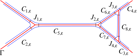
Figure 1: An example of a domain $\Omega_{\varepsilon}$ with four junctions, four unbounded channels and four bounded channels.

The domain $\Omega_{\varepsilon}$ shrinks to a one-dimensional metric graph $\Gamma$ as $\varepsilon\rightarrow 0$. The axes of the channels form edges $\Gamma_{j},$ $1\leq j\leq N,$ of $\Gamma$, and the distances between points of $\Gamma_{j}$ are defined by the distances between the corresponding points of the channels. The junctions shrink to vertices of the graph $\Gamma$. We denote the set of vertices $v_{j}$ by $V$.

Figure 2: Another example of a domain $\Omega_{\varepsilon}$, network of a necklace type which will be studied in more detail later.

For the sake of simplicity, we impose the following two geometrical conditions. First, we assume that all the channels $C_{j,\varepsilon}$ have the same cross-section $\pi_{\varepsilon}$ (the general case is studied in [23] ). The second condition concerns the junctions. We assume that they are self-similar. The latter means that there exist an $\varepsilon$- independent domain $J_{v}$ and a point $\widehat{x}=\widehat{x}_{v}$ such that

$$J_{v,\varepsilon}=\{(\widehat{x}+\varepsilon x):x\in J_{v}\}.$$ (2)

From the self-similarity assumption it follows that $\pi_{\varepsilon}\$is an $\varepsilon$-homothety of a bounded domain $\pi\subset R^{d-1}$.

Let $\lambda_{0}<\lambda_{1}\leq\lambda_{2}...$ be the eigenvalues of the negative Laplacian $-\Delta_{d-1}$ in $\pi$ with orthonormal eigenfunctions $\{\varphi_{n}(y)\}$,

$$-\Delta_{d-1}\varphi_{n}(y)=\lambda_{n}\varphi_{n}(y),~{}~{}Bu=0~{}~{}~{}\text{on}~{}~{}\partial\pi,$$

where $B$ is the boundary operator on the channels defined in (1). Then $\varepsilon^{-2}\lambda_{n}$ are eigenvalues of $-\Delta_{d-1}$ in $\pi_{\varepsilon}$ and $\{\varepsilon^{-d/2}\varphi_{n}(y/\varepsilon)\}$ are the corresponding orthonormal eigenfunctions,

$$-\Delta_{d-1}\varphi_{n}(y/\varepsilon)=\varepsilon^{-2}\lambda_{n}\varphi_{n}(y/\varepsilon),~{}~{}Bu=0~{}~{}~{}\text{on}~{}~{}\partial\pi_{\varepsilon.}$$

We will call the point $\varepsilon^{-2}\lambda_{0}$ the threshold, since it is the bottom of the absolutely continuous spectrum of operator (1) if $\Omega_{\varepsilon}$ has an infinite channel.

We introduce Euclidean coordinates $(z,y)$ in channels $C_{j,\varepsilon}$ chosen in such a way that the $z$-axis is parallel to the axis of the

Figure 3: Local coordinates in a channel.

channel, hyperplane $R_{y}^{d-1}$ is orthogonal to the axis, and $C_{j,\varepsilon}$ has the following form in the new coordinates:

$$C_{j,\varepsilon}=\{(z,\varepsilon y):0<z<l_{j},\text{ }y\in\pi\}.$$

If a channel $C_{j,\varepsilon}$ is bounded ($l_{j}<\infty$), the direction of the $z$ axis can be chosen arbitrarily (at least for now). If a channel is unbounded, then $z=0$ corresponds to its cross-section which is adjacent to the junction.

We will impose the condition $(\varepsilon\omega)^{2}\in(\lambda_{0},\lambda_{1})$ (see [23] for the general case). Note that waves governed by (1) do not propagate through the channels if $(\varepsilon\omega)^{2}<\lambda_{0}$. There exists only one propagating mode

$$e^{\pm i\sigma z}\varphi_{0}(y/\varepsilon),~{}~{}\sigma=\sqrt{\omega^{2}-\varepsilon^{-2}\lambda_{0}},$$ (3)

if $(\varepsilon\omega)^{2}\in(\lambda_{0},\lambda_{1})$, and there are many similar modes

$$e^{\pm i\sigma_{j}z}\varphi_{j}(y/\varepsilon),~{}~{}\sigma_{j}=\sqrt{\omega^{2}-\varepsilon^{-2}\lambda_{j}},$$

if $(\varepsilon\omega)^{2}>\lambda_{j}$.

While many particular cases of problem (1) with $(\varepsilon\omega)^{2}=\lambda_{0}+O(\varepsilon^{2})$ or $(\varepsilon\omega)^{2}<\lambda_{0}$ were considered (see references in [25]), the publications [22]-[25] were the first ones dealing with the case $(\varepsilon\omega)^{2}\geq\lambda_{0},\varepsilon\rightarrow 0,$ and the first ones where the significance of the scattering solutions for asymptotic analysis of $H_{\varepsilon}$ was established. In particular, it was shown there that in both cases $(\varepsilon\omega)^{2}>\lambda_{0}$ and $(\varepsilon\omega)^{2}\approx\lambda_{0},$ the scattering solutions for equation (1) and the resolvent of the operator $H_{\varepsilon}$ can be approximated by the corresponding solutions of the one-dimensional problem on the limiting graph $\Gamma$ with the GC expressed in terms of the scattering matrices of the individual extended junctions.

Let us recall the definition of scattering solutions for the problem (1) in $\Omega_{\varepsilon}$ when $(\varepsilon\omega)^{2}\in(\lambda_{0},\lambda_{1}).$ The scattering solution $\Psi=\Psi_{p,\varepsilon}$ describes the propagation of an incident wave with unit amplitude and frequency $\omega$ coming through the channel $C_{p,\varepsilon}$.

Definition 1

Let $\lambda_{0}<(\varepsilon\omega)^{2}<\lambda_{1}.$ A function $\Psi=\Psi_{p,\varepsilon},$ $1\leq p\leq m,$ is called a solution of the scattering problem in $\Omega_{\varepsilon}$ if

$$(-\Delta-\omega^{2})\Psi=0,\text{ \ }x\in\Omega_{\varepsilon};\text{ \ \ \ }B\Psi=0\text{ \ on }\partial\Omega_{\varepsilon},$$ (4)

and $\Psi$ has the following asymptotic behavior in infinite channels $C_{j,\varepsilon},\ \ 1\leq j\leq m:$

$$\Psi_{p,\varepsilon}=[\delta_{p,j}e^{-i\sigma z}+t_{p,j}e^{i\sigma z}]\varphi_{0}(y/\varepsilon)+O(e^{-\frac{\alpha z}{\varepsilon}}),~{}~{}z\rightarrow\infty,\text{ \ }\alpha>0.$$ (5)

Here $\sigma=\sqrt{\omega^{2}-\varepsilon^{-2}\lambda_{0}}$, $\delta_{p,j}$ is the Kronecker symbol, i.e. $\delta_{p,j}=1$ if $p=j,$ $\delta_{p,j}=0$ if $p$ $\neq j.$

Remark. The term with the coefficient $\delta_{p,j}$ in (5) corresponds to the incident wave (coming through the channel $C_{p,\varepsilon}$), $t_{p,p}$ is the reflection coefficient, the terms with coefficients $t_{p,j},j\neq p,$ describe the transmitted waves. The coefficients $t_{p,j}=t_{p,j}(\varepsilon,\omega)$ depend on $\varepsilon$ and $\omega$. The matrix

$$T=[t_{p,j}]$$ (6)

is called the scattering matrix.

Standard arguments based on the Green formula provide the following statement.

Theorem 2

When $\lambda_{0}<(\varepsilon\omega)^{2}<\lambda_{1},$ the scattering matrix $T$ is unitary and symmetric ($t_{p,j}=t_{j,p}$).

It happens that the scattering solutions $\Psi_{p,\varepsilon}$ can be approximated with an exponential in $\varepsilon$ accuracy using the scattering solutions of a one-dimensional problem on the limiting graph $\Gamma$ which are defined as follows. Consider the following equation on $\Gamma$

$$-\frac{d^{2}}{dz^{2}}\psi=\sigma^{2}\psi,~{}~{}\sigma=\sqrt{\omega^{2}-\varepsilon^{-2}\lambda_{0}}.$$ (7)

Obviously,

$$\psi=c_{1,j}e^{-i\sigma z}+c_{2,j}e^{i\sigma z}$$

on the edges $\Gamma_{j}\subset\Gamma$.

We split the set $V$ of vertices $v$ of the graph into two subsets $V=V_{1}\cup V_{2},$ where the vertices from the set $V_{1}$ have degree $1$ and correspond to the free ends of the channels, and the vertices from the set $V_{2}$ have degree at least two and correspond to junctions.

Definition 3

We will say that $\psi=\psi_{p,\varepsilon}$ is a solution of the scattering problem on the graph $\Gamma$ with the incident wave coming through the edge $\Gamma_{p}$ if $\psi_{p,\varepsilon}$ satisfies equation (7),

$$\psi_{p,\varepsilon}(\gamma)=\delta_{p,j}e^{-i\sigma z}+t_{p,j}e^{i\sigma z},~{}\gamma\in\Gamma_{j},$$ (8)

on infinite edges $\Gamma_{j},1\leq j\leq m$, and satisfies the following GC at vertices $v$ of $\Gamma$:

$$B\psi=0\text{ \ \ at }v\in V_{1},$$ (9)

$$i[I_{v}+T_{v}(\varepsilon\omega)]\frac{d}{dz}\psi^{(v)}(z)-\sigma[I_{v}-T_{v}(\varepsilon\omega)]\psi^{(v)}(z)=0,\text{ \ \ \ }z=0,\text{ \ \ \ }v\in V_{2}.$$ (10)

We keep the same BC at $v\in V_{1}$ as at the free end of the corresponding channel of $\Omega_{\varepsilon}$, see (1), and we will specify GC (10) in the next two paragraphs. However, first we would like to stress that scattering coefficients $t_{p,j}$ in (8) are not required to coincide with those defined in (5) for the problem in the domain $\Omega_{\varepsilon}$. With the appropriate choice of GC (10), these coefficients are the same, and therefore we use the same notation.

We choose the parametrization on $\Gamma$ in such a way that $z=0$ at $v$ for all edges adjacent to this particular vertex. Let $d=d(v)\geq 2$ be the order (the number of adjacent edges) of the vertex $v\in V_{2}.$ For any function $\psi$ on $\Gamma,$ we form a column-vector $\psi^{(v)}=\psi^{(v)}(z)$ with $d(v)$ components which is formed by the restrictions of $\psi$ on the edges of $\Gamma$ adjacent to $v.$ We will need this vector only for small values of $z\geq 0.$ The GC (10) are defined in terms of auxiliary scattering problems for extended junctions $J_{v,\varepsilon}^{\infty}$. Each extended junction consists of $J_{v,\varepsilon}$ and all the channels adjacent to $J_{v,\varepsilon}$. If some of these channels have finite length, we extend them to infinity (see Fig. 4).

Figure 4: An extended junction for a necklace waveguides.

The matrix $T=T_{v}(\varepsilon\omega)$ is the scattering matrix for the problem (1) in $J_{v,\varepsilon}^{\infty}$ and $I_{v}$ is the unit matrix of the same size as the size of $T.$ Note that the self-similarity of $J_{v,\varepsilon}^{\infty}$ implies that $T=T_{v}(\varepsilon\omega)$ depends only on the product $\varepsilon\omega$. Hence, $T_{v}$ can be determined by solving the scattering problem in the corresponding extended junction with $\varepsilon=1.$ Now (10) is defined. We need only to take components of the vector $\psi^{(v)}$ in the same order as the order of channels of $J_{v}^{\infty}.$

Denote by $F(\varepsilon)$ the set $\{\omega_{j}\}$ of the values of $\omega$ for which problem (7), (9), (10) has a nontrivial solution $\psi\in L^{2}(\Gamma)$ and $(\varepsilon\omega_{j})^{2}\in[\lambda_{0},\lambda_{1}]$. Note that both equation and the boundary conditions of the problem depend on $\omega$ and $\varepsilon$. Let $F^{0}$ be the set $\{\omega_{j}\}$ of values of $\omega$ such that $\omega_{j}^{2}$ is an eigenvalue of the operator $H_{\varepsilon}$ (see (1)) in one of the domains $J_{v,\varepsilon}^{\infty}$ and $(\varepsilon\omega_{j})^{2}\in[\lambda_{0},\lambda_{1}]$. Due to self-similarity of the extended junctions $J_{v,\varepsilon}^{\infty}$, the set $\varepsilon F^{0}$ does not depend on $\varepsilon$. Let $F^{\nu}$ be the $e^{\frac{-\nu}{\varepsilon}}$-neighborhood of the set $F^{0}\cup F(\varepsilon).$

Theorem 4

([25]) 1) The set $F^{0}\cup F(\varepsilon)$ has finitely many points (the number of points depends on $\varepsilon$).

2) For any interval $[\lambda_{0},\lambda^{\prime}],~{}\lambda^{\prime}<\lambda_{1},$ there exist $\rho,\nu>0$ such that scattering solutions $\Psi_{p,\varepsilon}(x)$ of the problem in $\Omega_{\varepsilon}$ have the following asymptotic behavior on the channels of $\Omega_{\varepsilon}$ as $\varepsilon\rightarrow 0$

$$\Psi_{p,\varepsilon}(x)=\psi_{p}^{(\varepsilon)}(\gamma)\varphi_{0}(\frac{y}{\varepsilon})+r_{p}^{(\varepsilon)}(x),~{}~{}\gamma\in\Gamma,$$

where $\psi_{p}^{(\varepsilon)}(\gamma)$ are the scattering solutions of the problem on the graph $\Gamma$ and

$$|r_{p}^{(\varepsilon)}(x)|\leq Ce^{\frac{-\rho d(\gamma)}{\varepsilon}},\text{ \ \ \ \ \ \ }(\varepsilon\omega)^{2}\in[\lambda_{0},\lambda^{\prime}],~{}\omega\notin F^{\nu}.$$

Here $\gamma=\gamma(x)$ is the point on $\Gamma$ which is defined by the cross-section of the channel through the point $x,$ and $d(\gamma)$ is the distance between $\gamma$ and the closest vertex of the graph.

Note that this theorem implies the coincidence of the scattering matrices of the problems on $\Omega_{\varepsilon}$ and on the graph $\Gamma$.

We will conclude this section by the following important proposition:

Proposition 5

Suppose that det$[I_{v}+T_{v}(\varepsilon\omega)]$ is not identically equal to zero. Then for all $\omega$ such that $~{}(\varepsilon\omega)^{2}\in[\lambda_{0},\lambda_{1}]$, except at most a finite number of points, the GC (10) can be written in the form

$$\frac{d}{dt}\psi^{(v)}(t)-\sigma A_{v}\psi^{(v)}(t)=0,~{}~{}t=0,~{}~{}\sigma^{2}=\sqrt{\omega^{2}-\varepsilon^{-2}\lambda_{0}},~{}~{}v\in V_{2},$$ (11)

where matrix

$$A_{v}=-i[I_{v}+T_{v}(\varepsilon\omega)]^{-1}[I_{v}-T_{v}(\varepsilon\omega)]$$

is real valued and symmetric ($A_{v}=A^{\prime}_{v}$).

Proof. Due to analyticity of $T_{v}$ in $\lambda$, we need only to justify properties of $A_{v}$. From Theorem 2 it follows that the eigenvectors of $T_{v}$ can be chosen to be real valued, i.e., there exists a real-valued orthogonal matrix $C_{v}=C_{v}(\lambda)$ such that $T_{v}=C_{v}^{-1}D_{v}C_{v}$ where $D_{v}$ is a diagonal matrix with elements $z_{j},~{}|z_{j}|=1$ on the diagonal. Numbers $z_{j}$ are (complex) eigenvalues of $T_{v}$. Obviously,

$$I_{v}\pm T_{v}=I_{v}\pm C_{v}^{-1}D_{v}C_{v}=C_{v}^{-1}[I_{v}\pm D_{v}]C_{v},~{}~{}A_{v}=iC_{v}^{-1}[I_{v}+D_{v}]^{-1}[I_{v}-D_{v}]C_{v}.$$

It remains to note that the numbers $i\frac{1-z_{j}}{1+z_{j}}$ are real.   

3 Necklace graphs

In this section we will consider a periodic metric graph $\Gamma$ of the necklace type (see [20]). It has the following form: one cell of periodicity consists of two arches $\mathcal{L}_{1},\mathcal{L}_{2}$ of lengths $l_{1}$ and $l_{2}\leq l_{1}$ connected at end points and of a segment $\mathcal{L}_{3}$ of length $l_{3}$ starting at one of these points (see fig. 1). We assume that the necklace is placed horizontally. Let $v_{2m-1},v_{2m}$ be the left and the right end points of the segments with $v_{0}$ being the origin, and with two arches connecting the points $v_{2m}$ and $v_{2m+1}$,    $m=0,\pm 1,\pm 2,...~{}.$

We introduce two related local coordinates $z$ and $s$ on the edges of the graph. Both are the lengths of the corresponding part of an arch or a segment, measured from some end of the edge. When a neighborhood of some vertex is considered (for example when GC are defined), the distance is measured from that vertex for all the edges adjacent to this vertex. The coordinate (distance) $z$ is used in this case. In other cases it will be convenient for us to measure the distance from the left end of the edge to the right. We will specify this situation by using parameter $s$ instead of $z$. Thus, $s=z$ or $s=l-z$ where $l$ is the length of the edge.

We equip the graph with the natural Lebesgue measure and consider the Hamiltonian $H$ on $L^{2}(\Gamma)$ given by $H=-\frac{d^{2}}{dz^{2}}=-\frac{d^{2}}{ds^{2}}$ on the graph with the following GC (see (11))

$$\frac{d}{dt}\psi^{(v)}(z)-\sigma A_{v}(\varepsilon\omega)\psi^{(v)}(z)=0,\text{ \ \ \ }z=0,\text{ \ \ \ }v\in V,$$ (12)

at the vertices of $\Gamma$. Here and below we use

$$\sigma=\sqrt{\omega^{2}-\varepsilon^{-2}\lambda_{0}}.$$

Our goal in this section is to study the propagation of waves on $\Gamma$ governed by the equation

$$H\psi=-\frac{d^{2}}{dz^{2}}\psi=\sigma^{2}\psi,~{}~{}\gamma\in\Gamma,$$ (13)

and GC (12). Note that both the equation and GC depend on the frequency $\omega$ and $\varepsilon$.

We enumerate the components $\psi_{j}$ of the vector $\psi^{(v)}$ in the following order: $\psi_{j}$ corresponds to the edge of the length $l_{j}$. Thus the first two components of the vector correspond to the shoulders of the loop, and the third component corresponds to the straight edge.

Figure 5: Graph $\Gamma$ for the necklace waveguide.

The goal of this section is to define and evaluate the (Prüffer) monodromy operator $M_{\sigma}$ (transfer operator over the period) for the problem (13), (12). Let $\psi^{\prime}=\frac{d\psi}{ds}$ and $\left(\begin{array}[]{c}\psi\\ \sigma^{-1}\psi^{\prime}\end{array}\right)(\alpha)$ be the Cauchy data (it always will have the factor $\sigma^{-1}$ in the second component) of the solution $\psi$ of the equation (13) evaluated at the point $\alpha$ of a straight segment of $\Gamma$. When $\alpha=v_{n}$ is one of the end points of a segment, we understand this vector as the limit of the corresponding vectors evaluated at $\alpha$ as $\alpha$ approaches $v_{n}$ moving along the segment (not along one of the arches). We denote by $M_{\sigma}$ the monodromy operator:

$$M_{\sigma}:\left(\begin{array}[]{c}\psi\\ \sigma^{-1}\psi^{\prime}\end{array}\right)(v_{0})\rightarrow\left(\begin{array}[]{c}\psi\\ \sigma^{-1}\psi^{\prime}\end{array}\right)(v_{2})$$

and we denote by $T_{\sigma}$ the (Prüffer) transfer operator over the loop:

$$T_{\sigma}:\left(\begin{array}[]{c}\psi\\ \sigma^{-1}\psi^{\prime}\end{array}\right)(v_{0})\rightarrow\left(\begin{array}[]{c}\psi\\ \sigma^{-1}\psi^{\prime}\end{array}\right)(v_{1}).$$

We will use the same notations $M_{\sigma},T_{\sigma}$ for the matrices of the operators as for the corresponding operators.

Let us write matrix $A_{v}=(a_{i,j})$ (see (11), (12)) in the form

$$A_{v}=\left(\begin{array}[]{c}B~{}\delta\\ \delta^{*}~{}c\end{array}\right),~{}~{}\text{where}~{}B=\left(\begin{array}[]{c}a_{1,1}~{}a_{1,2}\\ a_{2,1}~{}a_{2,2}\end{array}\right),~{}\delta=\left(\begin{array}[]{c}\delta_{1}\\ \delta_{2}\end{array}\right)=\left(\begin{array}[]{c}a_{1,3}\\ a_{2,3}\end{array}\right),~{}c=a_{3,3}.$$ (14)

We will need the following matrices

$$S=\left(\begin{array}[]{c}\sin\sigma l_{1}~{}~{}~{}~{}0\\ 0~{}~{}~{}~{}\sin\sigma l_{2}\end{array}\right),~{}~{}C=\left(\begin{array}[]{c}\cos\sigma l_{1}~{}~{}~{}~{}0\\ 0~{}~{}~{}~{}\cos\sigma l_{2}\end{array}\right),~{}~{}P=C+SB,$$ (15)

$$M=(I-P^{2})^{-1}PS,~{}~{}N=(I-P^{2})^{-1}S.$$ (16)

Theorem 6

1) Matrix $T_{\sigma}$ has the form

$$T_{\sigma}=-\left(\begin{array}[]{c}\frac{m}{n}~{}~{}~{}\frac{1}{n}\\ \frac{m^{2}-n^{2}}{n}~{}~{}\frac{m}{n}\end{array}\right),~{}~{}~{}n=\langle\delta,N\delta\rangle,~{}~{}m=c+\langle\delta,M\delta\rangle.$$ (17)

2) Matrix $M_{\sigma}$ has the form

$$M_{\sigma}=\left(\begin{array}[]{c}\cos\sigma l_{3}~{}~{}~{}\sin\sigma l_{3}\\ -\sin\sigma l_{3}~{}~{}~{}~{}\cos\sigma l_{3}\end{array}\right)T_{\sigma}.$$ (18)

Proof. Let $\psi_{j}=\psi_{j}(s),~{}j=1,2,$ be the restrictions of the function $\psi$ on the upper and lower arches of the graph between the points $v_{0}$ and $v_{1}$. Obviously,

$$\psi_{1}(s)=\frac{\psi_{1}(0)\sin\sigma(l_{1}-s)+\psi_{1}(l_{1})\sin\sigma s}{\sin\sigma l_{1}}.$$

Thus,

$$\psi_{1}^{\prime}(0)=\frac{-\sigma\psi_{1}(0)\cos\sigma l_{1}+\sigma\psi_{1}(l_{1})}{\sin\sigma l_{1}},~{}~{}\psi_{1}^{\prime}(l_{1})=\frac{-\sigma\psi_{1}(0)+\sigma\psi_{1}(l_{1})\cos\sigma l_{1}}{\sin\sigma l_{1}}.$$

A similar formula is valid for $\psi_{2}$. Hence, taking into account the relation between parameters $s$ and $t$, we obtain the following connection between the values of the vector $\phi=\left(\begin{array}[]{c}\psi_{1}\\ \psi_{2}\end{array}\right)$ and its derivative $\frac{d\phi}{dz}$ at points $v_{0}$ and $v_{1}$ of the graph:

$$\frac{d\phi}{dz}(v_{0})=-\sigma CS^{-1}\phi(v_{0})+\sigma S^{-1}\phi(v_{1}),~{}~{}\frac{d\phi}{dz}(v_{1})=-\sigma CS^{-1}\phi(v_{1})+\sigma S^{-1}\phi(v_{0}).$$

Let us denote the restrictions of $\psi$ on the straight edges of the graph by $\psi_{3}.$ Consider vectors $\psi^{(v_{0})}=\left(\begin{array}[]{c}\phi(v_{0})\\ \psi_{3}(v_{0})\end{array}\right),~{}\psi^{(v_{1})}=\left(\begin{array}[]{c}\phi(v_{1})\\ \psi_{3}(v_{1})\end{array}\right).$ GC (12) implies

$$\left(\begin{array}[]{c}-CS^{-1}\phi(v_{0})+S^{-1}\phi(v_{1})\\ \omega^{-1}\frac{d}{dz}\psi_{3}(v_{0})\end{array}\right)=\left(\begin{array}[]{c}B~{}~{}~{}\delta\\ \delta^{*}~{}~{}c\end{array}\right)\left(\begin{array}[]{c}\phi(v_{0})\\ \psi_{3}(v_{0})\end{array}\right),$$

$$\left(\begin{array}[]{c}-CS^{-1}\phi(v_{1})+S^{-1}\phi(v_{0})\\ \sigma^{-1}\frac{d}{dz}\psi_{3}(v_{1})\end{array}\right)=\left(\begin{array}[]{c}B~{}~{}~{}\delta\\ \delta^{*}~{}~{}c\end{array}\right)\left(\begin{array}[]{c}\phi(v_{1})\\ \psi_{3}(v_{1})\end{array}\right).$$

These equations can be rewritten in the following form

$$-(CS^{-1}+B)\phi(v_{0})+S^{-1}\phi(v_{1})=\delta\psi_{3}(v_{0}),$$

$$-\sigma^{-1}\frac{d}{ds}\psi_{3}(v_{0})=\delta^{*}\phi(v_{0})+c\psi_{3}(v_{0}),$$

$$-(CS^{-1}+B)\phi(v_{1})+S^{-1}\phi(v_{0})=\delta\psi_{3}(v_{1}),$$

$$\sigma^{-1}\frac{d}{ds}\psi_{3}(v_{1})=\delta^{*}\phi(v_{1})+c\psi_{3}(v_{1}).$$

We multiply the first and third equations by $S$, replace $C+SB$ by $P$ (see (15)) and then solve these equations for $\phi(v_{0}),~{}\phi(v_{1})$. This implies

$$\phi(v_{0})=-(I-P^{2})^{-1}PS\delta\psi_{3}(v_{0})+(I-P^{2})^{-1}S\delta\psi_{3}(v_{1}),$$

$$\phi(v_{1})=-(I-P^{2})^{-1}S\delta\psi_{3}(v_{0})+(I-P^{2})^{-1}PS\delta\psi_{3}(v_{1}).$$

We substitute these relations into the second and forth equations of the system above and then solve those equations for $\psi_{3}(v_{1}),~{}\sigma^{-1}\frac{d}{ds}\psi_{3}(v_{1})$. This provides the transfer operator over the loop with the transfer matrix defined in (17). This completes the proof of the first part of theorem. The second statement of the theorem is obvious, since the left factor in the right-hand side of (18) is the transfer matrix over the segment $[v_{0},v_{1}]$ of the graph.   

4 Some applications of necklace waveguides

We will discuss here two practical features of necklace waveguides. The first concerns slowing down of the light ( slowing down of propagation of wave packets) in these waveguides. There is an extended literature on the principles of this phenomenon, possible applications and practical devices. Usually some type of a periodic structure is suggested for these devices with a band-gap structure of the spectrum. If a narrow band is created, then the dispersion relation for the corresponding frequency is flat and the group velocity $V_{g}$ is small.

The main feature which distinguishes a necklace waveguide from other one-dimensional (or quasi one-dimensional) periodic problem is the following. While the Hill discriminant for a standard periodic Schrodinger operator is an analytic function of frequency, it is meromorphic for the necklace waveguides. We will show that one can easily find parameters when the Hill discriminant has two close poles (as close as one pleases) with a zero in between. Thus the band will be as narrow as we please around a chosen value $\sigma=\sigma_{0}$ of the frequency. Therefore, the group velocity will be small if the support of the wave packets belongs to a small neighborhood of $\sigma_{0}$.

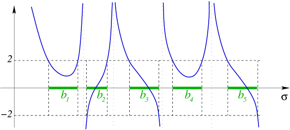
Figure 6: The graph of the Hill discriminant $\mathrm{Trace}M_{\sigma}=2\cos k(\sigma),~{}~{}\sigma=\sqrt{\omega^{2}-\varepsilon^{-2}\lambda_{0}}.$

The second feature concerns the truncated necklace graph (waveguide) $\Gamma_{N}$ which consists of $N$ cells of periodicity confined between points $v_{0}$ and $v_{2N}$ and the rays $(-\infty,v_{0}),(v_{2N},\infty.)$ When propagation of a narrow in frequency wave packet through a finite device is considered, it could happen that the waves, which are slowing down in the device, can not enter the device. In other words, one needs to know that the reflection coefficient $r$ for the truncated necklace waveguide is not too big (better if it is small) for the frequencies where the slowing down occurs. It will be shown that for a given frequency $\sigma=\sigma_{0}$ one can choose the parameters $l_{j},j=1,2,3,$ such that $V_{g}=r=0$ at $\sigma=\sigma_{0}$, and therefore they are small for $\sigma$ close enough to $\sigma_{0}$.

Slowing down, preliminary discussion. Theorem 4 allows us to reduce the study of propagation of single frequency waves and wave packets in periodic necklace waveguide $\Omega_{\varepsilon}$ (see Fig. 2) to a study of the corresponding problem on the necklace graph $\Gamma$ (see Fig. 5). One needs only to take in correspondence the frequencies $\omega$ and $\sigma$ of the waves in $\Omega_{\varepsilon}$ and on $\Gamma$ using the relation

$$\sigma=\sqrt{\omega^{2}-\varepsilon^{-2}\lambda_{0}}.$$

The spectrum of periodic problem (13), (12) has a band-gap structure with the bands on the $\sigma$-axis defined by the inequality

$$|F(\sigma)|<2,~{}~{}~{}F(\sigma)=\text{Tr}M_{\sigma},$$

where function $F$ (called the Hill discriminant) is equal to the trace of the monodromy matrix (see Fig 6). The same function defines the dispersion relation (we will write it in the form $k=k(\sigma)$) of the problem on $\Gamma$:

$$\cos k(\sigma)=\frac{1}{2}F(\sigma)=\frac{1}{2}\text{Tr}M_{\sigma}.$$ (19)

Let $\omega=\omega_{0}$ belong to the frequency interval of a narrow wave packet of the problem in $\Omega_{\varepsilon}$ and

$$\sigma_{0}=\sqrt{\omega_{0}^{2}-\varepsilon^{-2}\lambda_{0}}.$$

We will find parameters $l_{j}$ in such a way that

$$|F(\sigma_{0})|=0,$$ (20)

and there is a point $\sigma=\sigma_{1}$, for example, to the right of $\sigma_{0}$, such that $F(\sigma)$ has a pole at $\sigma=\sigma_{1}$ and $|\sigma_{0}-\sigma_{1}|=\epsilon\ll 1$. Then there is a point $\sigma^{\prime}\in(\sigma_{0},\sigma_{1})$ such that

$$|F(\sigma)|<1~{}~{}\text{for}~{}~{}\sigma\in\Delta=(\sigma_{0},\sigma^{\prime}),~{}~{}|F(\sigma^{\prime})|=1.$$

Then interval $\Delta$ belongs to a band. From (19) it follows that $k(\sigma)$ changes by $\pi/6$ between $\sigma_{0}$ and $\sigma^{\prime}$. Hence, $k^{\prime}(\sigma)=O(1/\epsilon)$ on $\Delta$ or on some part $\Delta^{\prime}$ of $\Delta$, i.e.,

$$V_{g}=\frac{L}{k^{\prime}(\sigma)}=O(\epsilon),~{}~{}\sigma\in\Delta^{\prime}.$$ (21)

Note that matrix $T_{\sigma}$ has a pole if $n=0$. Since matrices $T_{\sigma}$ and $M_{\sigma}$ differ by a rotation, one can easily choose $l_{3}$ such that $F(\sigma)=\frac{1}{2}$Tr$M_{\sigma}$ has a pole at a point where $n=0$ (in fact, the pole of $F(\sigma)$ exists for all but specific values of $l_{3}$). Thus the following equation provides the poles of $F(\sigma)$ under an appropriate choice of $l_{3}$ (see (15)-(17))

$$n=\langle\delta,(I-P^{2})^{-1}S\delta)\rangle=\frac{1}{2}\langle\delta,[(I-P)^{-1}+(I+P)^{-1}]S\delta)\rangle=0,~{}~{}P=C+SB.$$

Let us introduce the matrix

$$T=\frac{I-C}{S}=\left(\begin{array}[]{c}x~{}~{}0\\ 0~{}~{}y\end{array}\right),~{}~{}~{}x=\tan\frac{\sigma l_{1}}{2},~{}~{}y=\tan\frac{\sigma l_{2}}{2}.$$ (22)

Then the equation $n=0$ can be rewritten in the form

$$2n=\langle\delta,[(T-B)^{-1}+(T^{-1}+B)^{-1}]\delta)\rangle=0.$$ (23)

We will conclude this subsection by an re-writing (23) using the components of matrix $B$ and vector $\delta$ (see (14)):

$$2n=\frac{(y-a_{2,2})\delta_{1}^{2}+(x-a_{1,1})\delta_{2}^{2}+2a_{1,2}\delta_{1}\delta_{2}}{(x-a_{1,1})(y-a_{2,2})-a_{1,2}^{2}}$$

$$+\frac{(y^{-1}+a_{2,2})\delta_{1}^{2}+(x^{-1}+a_{1,1})\delta_{2}^{2}-2a_{1,2}\delta_{1}\delta_{2}}{(x^{-1}+a_{1,1})(y^{-1}+a_{2,2})-a_{1,2}^{2}}=0.$$ (24)

This is an algebraic equation of the forth order with respect to $(x,y)$. We will discuss it in more detail later.

Transparency, preliminary discussion. Let us recall the estimate (see [21]) for the reflection coefficient $r=r_{N}$ by a finite slab of periodic media which consists of $N$ periods:

$$|r_{N}|=|\frac{\sin Nk(\sigma)}{\sin k(\sigma)}|(||M_{\sigma}||^{2}-2)^{1/2},$$ (25)

where $||M_{\sigma}||$ is the Gilbert-Shmidt norm of the monodromy matrix, i.e.

$$||M_{\sigma}||^{2}=||(m_{i,j})||^{2}=\sum_{i,j\leq 2}m_{i,j}^{2}.$$

We will choose parameters $l_{j}$ in such a way that the frequency support $\Delta$ of the wave packet is in the middle of a band where $|F(\sigma)|<1$. Then $|\sin k(\sigma)|>\frac{\sqrt{3}}{2}$ there, and

$$|r_{N}(\sigma)|=\frac{2}{\sqrt{3}}|(||M_{\sigma}||^{2}-2)^{1/2},~{}~{}\sigma\in\Delta.$$ (26)

We will choose $l_{1},~{}l_{2}$ in such a way that $||M_{\sigma_{0}}||^{2}=2$ , and therefore

$$r_{N}(\sigma_{0})=0.$$ (27)

Then $r_{N}(\sigma)$ is small in a small neighborhood of $\sigma_{0}$, and we will have both the slowing down of the light and the transparency in $\Delta^{\prime}$.

Note that $||M_{\sigma}||=||T_{\sigma}||$ (see (18)) and that det$T_{\sigma}=1$. Thus $||T_{\sigma}||\geq 2$ and $||T_{\sigma}||=2$ if matrix $T_{\sigma}$ is orthogonal (the sum of its off-diagonal elements is zero). Hence, condition

$$(m+n)(m-n)+1=m^{2}-n^{2}+1=0$$ (28)

provides (27). We are going to write this condition more explicitly.

From (16), (17) it follows that

$$m+n=c+\langle\delta,(I-P)^{-1}S\delta\rangle=c+\langle\delta,[S^{-1}(I-C-SB)]^{-1}\delta\rangle=c+\langle\delta,[(T-B)]^{-1}\delta\rangle,$$

where $T$ is defined in (22). Similarly

$$m-n=c-\langle\delta,(I+P)^{-1}S\delta\rangle=c-\langle\delta,[S^{-1}(I+C+SB)]^{-1}\delta\rangle=c-\langle\delta,[(T^{-1}+B)]^{-1}\delta\rangle.$$

We substitute the last two formulas into (28) and obtain the following exact form for (27):

$$[c+\frac{(y-a_{2,2})\delta_{1}^{2}+(x-a_{1,1})\delta_{2}^{2}+2a_{1,2}\delta_{1}\delta_{2}}{(x-a_{1,1})(y-a_{2,2})-a_{1,2}^{2}}]\cdot$$

$$\cdot[c-\frac{(y^{-1}+a_{2,2})\delta_{1}^{2}+(x^{-1}+a_{1,1})\delta_{2}^{2}-2a_{1,2}\delta_{1}\delta_{2}}{(x^{-1}+a_{1,1})(y^{-1}+a_{2,2})-a_{1,2}^{2}}]+1=0.$$ (29)

Thus, the set of transparency points $\{r_{N}=0\}$ is also given by zeroes of a polynomial of forth order in $(x,y)$-plane, $x=\tan\frac{\sigma l_{1}}{2},~{}y=\tan\frac{\sigma l_{2}}{2}$. To be more accurate, we need to omit points where $n=0$ from this set, since (28) provides the orthogonality of $T_{\sigma}$ only if $n\neq 0$.

The choice of parameters. The center $\sigma_{0}$ in the frequency interval of the wave packet is given. We need to choose $l_{1},~{}l_{2}$ in such a way that (27)-(29) hold at $\sigma_{0}$ and this point is close to a point where (24), (23) hold. Note that condition (27) is equivalent to the orthogonality of matrix $T_{\sigma_{0}}$. Then one can easily transfer it by rotation to a matrix with zero trace, i.e., one can find $l_{3}$ such that (20) holds. Hence, it remains to choose $l_{1},~{}l_{2}$ appropriately.

We note that equation (28) for $\sigma_{0}$ contradicts the condition $n=0$ imposed by (24), (23). Moreover, $n$ can not vanish at a point close to $\sigma_{0}$ if $n$ is smooth. In order for equation (28) to be valid at a point $\sigma_{0}$ and $n$ to be zero at $\sigma_{1}$ which is close to $\sigma_{0}$, function $n$ has to be singular near $\sigma_{0}$. Thus one must choose parameters $(x,y)$ near the point where one of the denominators in (24) is zero. Let us choose the denominator of the first fraction. Then the numerator of the first fraction also must be small (otherwise (24) is not valid at $\sigma=\sigma_{1}$). By equating both the numerator and the denominator of the first fraction in (24) to zero we find that

$$x\approx a_{1,1}-a_{1,2}\frac{\delta_{1}}{\delta_{2}},~{}~{}y\approx a_{2,2}-a_{1,2}\frac{\delta_{2}}{\delta_{1}}.$$

Finally, we fix small $\epsilon$ and choose

$$x=a_{1,1}-a_{1,2}\frac{\delta_{1}}{\delta_{2}}+\epsilon.$$ (30)

Then we solve (29) for $y$ in a neighborhood of the point $a_{2,2}-a_{1,2}\frac{\delta_{2}}{\delta_{1}}$. This implies

$$y=a_{2,2}-a_{1,2}\frac{\delta_{2}}{\delta_{1}}-(\frac{\delta_{2}}{\delta_{1}})^{2}\epsilon+\gamma\epsilon^{2}+\text{O}(\epsilon)^{3},$$ (31)

where the exact value of $\gamma$ can be easily found from (29). We put $\sigma=\sigma_{0}$ in (22) and determine $l_{1},~{}l_{2}$ from (30), (31). This choice of $l_{1},~{}l_{2}$ implies (27).

By solving (24) asymptotically, we find that its solution also has the form (30), (31) with a different value of $\gamma$. This justifies the existence of a pole of the Hill discriminant at the distance O$(\epsilon^{2})$ from the point $\sigma_{0}.$ In fact, let us omit the cubic term in (31). Then equations (30), (31) with two different values of $\gamma$ define two parabolas $P_{1}$ and $P_{2}$ with the same vertex and tangent line at the vertex. If we put $\sigma=\sigma_{0}$ in (22) and fix $\epsilon$, we get a point on $P_{1}$ at the distance of order $\epsilon$ from the vertex which defines $l_{1},l_{2}$. This choice implies (27). When $\sigma$ changes: $\sigma=\sigma_{0}+\tau,~{}0\leq\tau\leq\tau_{0}$, point $(x,y)$ moves in the direction of the vector $(l_{1},l_{2})$ or in the opposite direction (see 22). We may change the sign of $\tau$, if needed, to guarantee that the point moves toward the second parabola where $n=0$. The only unacceptable situation is when the vector $(l_{1},l_{2})$ is tangent to $P_{1}$. It will not happen in a generic case. Besides one can always avoid it by changing $l_{1}$ or $l_{2}$, since they are defined up to an integer multiple of $2\pi$.

The arguments above prove that wave packet with frequencies in O$(\epsilon^{2})$-semi-neighborhood of $\sigma_{0}$ will propagate with the group velocity $V_{g}=$O$(\epsilon^{2})$ and the reflection coefficient will have order O$(\epsilon^{2})$.

We conclude this subsection by the following remark. Let the geometry of the junctions be chosen. After that, we must choose specific $l_{1},l_{2}$ satisfying (30), (31). It is easy to choose one of these parameters (for example, $l_{1}$) by changing the distance between two neighboring junctions, but $l_{2}$ will be defined after that by the geometry of the network. In fact it is not the geometrical, but only the optical length which plays role here. One can preserve the geometry of the network and change the refraction index in some of the channels to satisfy the relations (30), (31). This produces the same effect as changing the lengths of the corresponding channels.

Acknowledgment. The authors were supported partially by the NSF grant DMS-0706928.

References

• [1] Dell’Antonio, G., Tenuta, L.: Quantum graphs as holonomic constraints, J. Math. Phys., 47 (2006), 072102:1-21.
• [2] Duclos P., Exner, P.: Curvature-induced bound states in quantum waveguides in two and three dimensions, Rev. Math. Phys., 7 (1995), 73-102.
• [3] Duclos P., Exner P., Stovicek P.: Curvature-induced resonances in a two-dimensional Dirichlet tube, Ann. Inst. H. Poincare 62 (1995), 81-101.
• [4] Exner P., Post O.: Convergence of spectra of graph-like thin manifolds, J. Geom. Phys., 54 (2005), 77-115.
• [5] Exner P., Ε eba P.: Electrons in semiconductor microstructures: a challenge to operator theorists, in SchrΓΆdinger Operators, Standard and Nonstandard (Dubna 1988), World Scientific, Singapure (1989), 79-100.
• [6] Exner P. and Ε eba P.: Bound states in curved quantum waveguides, J. Math. Phys. 30(1989), 2574 - 2580.
• [7] Exner P., Ε eba P.: Trapping modes in a curved electromagnetic waveguide with perfectly conducting walls, Phys. Lett. A144 (1990), 347-350.
• [8] Exner P. and Vugalter S. A.: Asymptotic estimates for bound states in quantum waveguides coupled laterally through a narrow window, Ann. Inst. H. Poincare, Phys. Theor. 65 (1996), 109 - 123.
• [9] Exner P. and Vugalter S. A.: On the number of particles that a curved quantum waveguide can bind, J. Math. Phys. 40 (1999), 4630-4638.
• [10] Exner P., Weidl T.: Lieb-Thirring inequalities on trapped modes in quantum wires, Proceedings of the XIII International Congress on Mathematical Physics (London 2000), International Press of Boston, 2001, pp.437-443.
• [11] Freidlin M., A. Wentzel A.: Diffusion processes on graphs and averaging principle, Ann. Probab., Vol 21, No 4 (1993), 2215-2245.
• [12] Freidlin M.: Markov Processes and Differential Equations: Asymptotic Problems, Lectures in Mathematics, ETH Zurich, Birkhauser Verlag, Basel, 1996.
• [13] Kostrykin V., Schrader R.: Kirchhoff’s rule for quantum waves, J. Phys. A: Mathematical and General, Vol 32 (1999), 595-630.
• [14] Kuchment P.: Graph models of wave propagation in thin structures, Waves in Random Media, Vol.12 (2002), 1-24.
• [15] Kuchment P.: Quantum graphs. I. Some basic structures, Waves in Random Media, Vol.14, No 1 (2004), 107-128.
• [16] Kuchment P.: Quantum graphs. II. Some spectral properties of quantum and combinatorial graphs, Journal of Physics A: Mathematical and General, Vol 38, No 22 (2005), 4887-4900.
• [17] Kuchment P., Zeng H.: Convergence of spectra of mesoscopic systems collapsing onto a graph, J. Math. Anal. Appl. 258 (2001), 671-700.
• [18] Kuchment P., Zeng H.: Asymptotics of spectra of Neumann Laplacians in thin domains, in Advances in Differential Equations and mathematical Physics, Yu. Karpeshina etc (Editors), Contemporary Mathematics, AMS, 387 (2003), 199-213.
• [19] S. Molchanov, B. Vainberg, Β Slowdown of the wave packet in finite slabs of periodic media, Waves in Random Media, 14 (2004), 411-423.
• [20] S. Molchanov, B. Vainberg, Β Slowing down of wave packets in quantum graphs, Waves in Complex and Random Media, 15, No 1 (2005), 101-112.
• [21] S. Molchanov, B. Vainberg, Β Slowing down and reflection of waves in trancated periodic media, J. of Funct. Analysis, 231 (2006), 287-311.
• [22] Molchanov S. and Vainberg B.: Transition from a network of thin fibers to quantum graph: an explicitly solvable model, Contemporary Mathematics, 415, AMS (2006), 227-240 (arXiv:math-ph/0605037).
• [23] Molchanov S. and Vainberg B.: Scattering solutions in networks of thin fibers: small diameter asymptotics, Comm. Math. Phys., 273, N2, (2007), 533-559 (arXiv:math-ph/0609021).
• [24] Molchanov S. and Vainberg B.: Laplace operator in networks of thin fibers: spectrum near the threshold, inΒ Stochastic analysis in mathematical physics, 69–93, World Sci. Publ., Hackensack, NJ, 2008 (arXiv:0704.2795).
• [25] Molchanov S. and Vainberg B.: Propagation of Waves in Networks of Thin Fibers, submitted
• [26] Mikhailova, A., Pavlov, B., Popov, I., Rudakova, T., Yafyasov, A.: Scattering on a compact domain with few semi-infinite wires attached: resonance case. Math. Nachr. 235 (2002), 101–128.
• [27] Pavlov B., Robert K.: Resonance optical switch: calculation of resonance eigenvalues. Waves in periodic and random media (South Hadley, MA, 2002), 141–169, Contemp. Math., 339, Amer. Math. Soc., Providence, RI, 2003.
• [28] Post O.: Branched quantum wave guides with Dirichlet BC: the decoupling case, Journal of Physics A: Mathematical and General, Vol 38, No 22 (2005), 4917-4932.
• [29] Post O.: Spectral convergence of non-compact quasi-one-dimensional spaces, Ann. Henri Poincar, 7 (2006), 933-973.
• [30] Rubinstein J., Schatzman M.: Variational problems on multiply connected thin strips. I. Basic estimates and convergence of the Laplacian spectrum, Arch. Ration. Mech. Anal., 160 (2001), No 4, 293-306.