Inferring genetic networks: an information theoretic approach

Abstract

In the postgenome era many efforts have been dedicated to systematically elucidate the complex web of interacting genes and proteins. These efforts include experimental and computational methods. Microarray technology offers an opportunity for monitoring gene expression level at the genome scale. By recourse to information theory, this study proposes a mathematical approach to reconstruct gene regulatory networks at coarse-grain level from high throughput gene expression data. The method provides the a posteriori probability that a given gene regulates positively, negatively or does not regulate each one of the network genes. This approach also allows the introduction of prior knowledge and the quantification of the information gain from experimental data used in the inference procedure. This information gain can be used to chose genes to be perturbed in subsequent experiments in order to refine the knowledge about the architecture of an underlying gene regulatory network. The performance of the proposed approach has been studied by in numero experiments. Our results suggest that the approach is suitable for focusing on size-limited problems, such as, recovering a small subnetwork of interest by performing perturbation over selected genes.

Introduction

Gene expression is regulated by proteins that enhance or block polymerase binding at the promoter region. These biochemical reactions constitute the edges of the gene regulatory networks. One of the key issues in modern biology is the elucidation of the structure and function of gene regulatory circuits at the system level hood . To address this challenge many efforts have been devoted to the task of developing computational methods capable of inferring the interaction between genes from expression levels both on small pathways luna ; jjc as on genome-wide scale (see rev1 for a review). Several models for gene regulatory networks have been proposed in order to infer network interactions holter ; tegner , such as Bayesian networks friedman ; husmeier ; beal , Boolean networks akutsu , linear model dhaeseleer1 ; dhaeseleer2 ; vansomeren . Once a regulatory network model has been chose, it is possible, in principle, to recover its parameters with some accuracy. Of course, more detailed models will require more extensive experimental data. In general this data is not available for the genome-wide scale assuming complex model. However, we can concentrate on simpler task, such as: who is regulating whom? and, Is that an up-regulation or a down-regulation? The idea behind restricting our questions at this qualitative information level, is to reduce the amount of data needed to infer valuable and robust biological knowledge even when dealing with noise data. In any case, the detailed information offered by more detailed modeling is not useful without a careful significance analysis of these predictions. In this sense, this study proposes a mathematical approach to infer gene networks at the coarse grain level. The inference process is to be accomplished according to Ockham’s razor, i.e., with the minimum number of assumptions compatible with the available data. To do that, the information theory (IT) is used within the framework of the maximum entropy principle sh ; j . IT has proved to be of utility in devising techniques for analyzing gene expression and network reconstruction lezon ; martinez , where gene expression levels were regarded as random variables. Here, complementing these previous works, each putative interaction has been considered as a random variable. In numero experiments show that, in this case, the IT parlance also provides a powerful framework to discuss questions related to the modeling process such as: (i) how to incorporate a priori information about the gene interaction; (ii) how to asses the likelihood of the inferred paths; (iii) how to quantify the information provided by the experimental data; and (iv) how to design experiments in order to identify subnetworks.

The IT approach

In general a genetic network can be modeled by a set of non-linear differential equations $\dot{x}_{i}=f_{i}\left(x_{1}(t),\ldots,x_{N}(t)\right)$, where $x_{i}(t)$ is the expression level of gene $i$ at time $t$ and $f_{i}$ is the regulatory function governing the expression of gene $i$ yang . Near a steady state the nonlinear system can be approximated by a set of linear differential equations, $\dot{{\bf x}}={\bf W}{\bf x}$ where ${\bf W}$, is a weighted connectivity matrix yeung . In order to uncover the connectivity matrix, we can apply a stimulus ${\bf b}=\left(b_{1}(t),\ldots,b_{N}(t)\right)^{T}$, then measure simultaneously the mRNA levels relative to $N$ genes ${\bf x}$ and estimate the derivative $\dot{\bf x}$. Repeating the procedure $M$ times we get a measurement matrix ${\bf X}$ where columns denote the experiments and where rows indicate individual genes. Thus, we can approximate the dynamics by

$$\dot{{\bf X}}={\bf W}\ {\bf X}+{\bf B}$$ (1)

where $\dot{\bf X}$ and ${\bf B}$ follow the same notation as ${\bf X}$.

Usually, inferring genetic network attempts to retrieve the weight matrix ${\bf W}$, where the elements $w_{ij}$ describe the type and strength of influence of gene $j$ on gene $i$ ($w_{ij}>0$ indicates activation, $w_{ij}>0$ indicates repression, and a zero indicates no influence). However, without a careful assessment of the significance of the weight-values, this could lead to the conclusion that the network is fully connected in contradiction to the well-known fact that gene regulatory networks are sparse networks.

In the present work, the maximum entropy principle is applied to obtain the probability distribution from the data $D_{M}=\left\{{\bf X,\dot{X},B}\right\}$, over the possible matrix ${\bf W}$. After that, using maximum likelihood criterion, the gene interaction matrix ${\bf I}$ is selected. The elements $I_{ij}$ can take only three values, depending on the type of influence of gene $j$ on gene $i$, $I_{ij}=1$ for activation (direct or indirect), $I_{ij}=-1$ for repression and $I_{ij}=0$ when gene $j$ does not have influence on gene $i$. In order to infer weights consistent with $D_{M}$, it is assumed that each set of weights ${\bf W}$ is realized with probability $P\left({\bf W}|D_{M}\right)$. In other words, a normalized probability distribution is introduced over the possible sets ${\bf W}$, which satisfy

$$\langle{\bf W}\rangle=\int P\left({\bf W}|D_{M}\right){\bf W}d{\bf W}.$$ (2)

The relative entropy related to an a priori probability distribution $P_{0}$, is given by

$$H_{r}\left(D_{M}\right|P_{0})=-\int P\left({\bf W}|D_{M}\right)\ln\left[\frac{P\left({\bf W}|D_{M}\right)}{P_{0}({\bf W})}\right]d{\bf W},$$ (3)

where $P_{0}\left({\bf W}\right)$ is an appropriate a priori distribution. The negative relative entropy $H_{r}$, known as Kullback-Leibler distance lt , defines the information gained after $D_{M}$ has been used in the inference procedure. Thus, in this framework, the inference process takes place through a modification of the probability distribution on weights space due to incoming data.

Among all possible distributions $P\left({\bf W}|D_{M}\right)$ consistent with $D_{M}$, $P\left({\bf W}|D_{M}\right)$ has been selected which comprises no unjustified prejudice. Thus, following the central tenets of the maximum entropy principle, relative entropy is maximized subject to the constraints Eq. 2. Thus, the a posteriori probability distribution yields,

$$P\left({\bf W}|D_{M}\right)=\exp\left(-\left(1+\lambda_{0}\right)\right)\exp\left(-{\bf W}\cdot{\bf\Gamma}\right)P_{0}\left({\bf W}\right),$$ (4)

where $\lambda_{0}$ is Lagrange multiplier associated to the normalization condition, and ${\bf\Gamma}$ the Lagrange multipliers associated to the constraints Eq. 2, which are determined once $P_{0}$ is properly selected.

In order to select $P_{0}$, it is assumed that the weights are restricted to the values of $I_{ij}$ i.e. $w_{ij}=0,\pm 1$ and then a three-peaked a priori distribution is used, which is described by

$$P_{0}\left({\bf W}\right)= (2\pi a)^{-N/2}\prod_{ij}^{N}\left[p_{ij}^{0}e^{-\frac{w_{ij}^{2}}{2a}}+p_{ij}^{+}e^{-\frac{\left(w_{ij}-1\right)^{2}}{2a}}+\right.$$ (5)

$$+ \left.p_{ij}^{-}e^{-\frac{\left(w_{ij}+1\right)^{2}}{2a}}\right],$$

where $p_{i,j}^{\rm x}$ is the a priori probability for gene $j$ to regulate positively (${\rm x}=+$), negatively (${\rm x}=-$) or to not regulate (${\rm x}=0$) gene $i$. Of course $p_{ij}^{0}+p_{ij}^{+}+p_{ij}^{-}=1$ for each pair $i,j$. The parameter $a$ can be regarded as a constraint smoothness parameter. Replacing this choice in Eq. 4 the a posteriori probability distribution is obtained as a sum of three Gaussians,

$$P\left({\bf W}|D_{M}\right)=\frac{1}{(2\pi a)^{N/2}}\prod_{ij}^{N}\left[\hat{p}_{ij}^{0}\ e^{-\frac{\left(w_{ij}+a\Gamma_{ij}\right)^{2}}{2a}}+\right.$$

$$\left.+\hat{p}_{ij}^{+}\ e^{-\frac{\left(w_{ij}+a\Gamma_{ij}-1\right)^{2}}{2a}}+\hat{p}_{ij}^{-}\ e^{-\frac{\left(w_{ij}+a\Gamma_{ij}+1\right)^{2}}{2a}}\right]$$ (6)

where $\hat{p}_{ij}^{\rm x}$ is the a posteriori probability for gene $j$ regulate positively (${\rm x}=+$), negatively (${\rm x}=-$) or to not regulate (${\rm x}=0$) gene $i$. These probabilities are defined by $\hat{p}_{ij}^{+}=p_{ij}^{+}e^{-\Gamma_{ij}}/z_{ij}$, $\hat{p}_{ij}^{-}=p_{ij}^{-}e^{\Gamma_{ij}}/z_{ij}$ and $\hat{p}_{ij}^{0}=p_{ij}^{0}/z_{ij}$, where $z_{ij}=1+p_{ij}^{+}\left(e^{-\Gamma_{ij}}-1\right)+p_{ij}^{-}\left(e^{\Gamma_{ij}}-1\right)$ guarantee normalization. Furthermore, the relative entropy of the a posteriori distribution Eq. 3 is given by

$$H_{r}\left(D_{M},P_{0}\right)=-\sum_{i}^{N}I_{g}\left(i|D_{M},P_{0}\right),$$ (7)

where $I_{g}(i)$ is the information gain of gene $i$ with respect to $P_{0}$ obtained from using the data $D_{M}$ which is defined by

$$I_{g}\left(i|D_{M},P_{0}\right) = \sum_{j}^{N}\left[\frac{a}{2}\Gamma^{2}_{ij}-\ln\left(z_{ij}\right)-\right.$$ (8)

$$\left.\frac{1}{z_{ij}}\left(p_{ij}^{+}\Gamma_{ij}e^{-\Gamma_{ij}}-p_{ij}^{-}\Gamma_{ij}e^{\Gamma_{ij}}\right)\right].$$

The multipliers $\Gamma_{ij}$ are obtained after solving the equation

$$\langle w_{ij}\rangle=-a\Gamma_{ij}+z_{ij}^{-1}\left(p_{ij}^{+}e^{-\Gamma_{ij}}-p_{ij}^{-}e^{\Gamma_{ij}}\right).$$ (9)

where $\langle w_{ij}\rangle$ are subject to the constraints imposed by $D_{M}$. Our central idea is that of reinterpreting, following the information in $D_{M}$ in a particular fashion,

$$\dot{{\bf X}}-{\bf B}=\langle{\bf W}\rangle\ {\bf X}.$$ (10)

Thus, all of the possible networks that are consistent with Eq. 10, can be written as

$$\langle{\bf W}\rangle=\left(\dot{{\bf X}}-{\bf B}\right)\cdot{\bf U}\cdot{\rm diag}(s_{j}^{-1})\cdot{\bf V}^{T}+{\bf C}\cdot{\bf V}^{T}$$ (11)

${\bf C}=(c_{ij})$ is an $N\times N$ matrix, where $c_{ij}$ is zero if $s_{j}\neq 0$ and is otherwise an arbitrary scalar coefficient. ${\bf U}$, ${\bf S}$ and ${\bf V}$ correspond to the singular value decomposition of matrix ${\bf X}^{T}$, i.e. ${\bf X}^{T}={\bf U}\cdot{\bf S}\cdot{\bf V}^{T}$ where ${\bf U}$ is a unitary $M\times N$ matrix of left eigenvectors, ${\bf S}$ is diagonal $N\times N$ matrix containing the eigenvalues $\left\{s_{1},\ldots,s_{N}\right\}$, and ${\bf V}$ is a unitary $N\times N$ matrix of right eigenvectors. Without loss of generality, let all non-zero elements of $s_{j}$ be listed at the end and $s_{j}^{-1}$ in Eq. 11 are taken to be zero if $s_{j}=0$. The general solution 11 can be written as

$$\langle{\bf W}\rangle={\bf W}_{L_{2}}+{\bf C}\cdot{\bf V}^{T}$$ (12)

where ${\bf W}_{L_{2}}$ is the particular solution with the smallest $L_{2}$ norm. If $M<N$, many weights ${\bf W}$ are compatible with the available information. The information contained in the data set $D_{M}$ can be used in different ways. Each of these leads to a different probability distribution which exhibits diverse properties. In this sense, following the prescription $\langle{\bf W}\rangle=0$ in Eq. 12, the knowledge that gene regulatory networks are sparse can be made use of. Thus, we have ${\bf C}\cdot{\bf V}^{T}=-{\bf W}_{L_{2}}$, which is an overdetermined problem yeung . This particular solution will be denoted as ${\bf W}_{L_{1}}$. Of course the ${\bf\Gamma}$ is obtained solving Eq. 9 using $\langle{\bf W}\rangle={\bf W}_{L_{2}}$ or $\langle{\bf W}\rangle={\bf W}_{L_{1}}$. In the following sections these alternatives will be considered independently. Notice that for $M\geq N$, ${\bf W}_{L_{2}}={\bf W}_{L_{1}}$.

After determining the a posteriori distribution, the gene interaction matrix $I$ must be selected. In order to do that, the maximum likelihood criterion is taken into account, i.e. the selection is accomplished choosing the highest a posteriori probability from $\{\hat{p}_{ij}^{0},\hat{p}_{ij}^{+},\hat{p}_{ij}^{-}\}$ for each pair $i,j$. For example if $\hat{p}_{ij}^{+}$ is greater than $\hat{p}_{ij}^{0}$ and $\hat{p}_{ij}^{-}$, then $I_{ij}=1$ indicating that gene $j$ activates the gene $i$.

In order to achieve the best model, the idea is to use the information contained in $D_{M}$ and the knowledge that gene regulatory networks are sparse. The formalism presented here offers an alternative to the prescription which selects ${\bf W}_{L_{1}}$ from all possible solutions 11. This alternative consists in setting $p_{ij}^{+}=p_{ij}^{-}\ll p_{ij}^{0}$. In this way the knowledge that gene regulatory network is sparse can be introduced by assigning a much lower value to the a priori probabilities of interaction than the a priori probabilities of absence of interaction. Furthermore, as the inference processes occur row by row, any other relevant a priori information about the gene in consideration (such as known interactions, type of gene, etc.) could be included in these probabilities. For example, if gene $k$ encode a helix-turn-helix or a zinc finger protein, high probabilities can be assigned for column $k$ ($p_{ik}^{+}$ and $p_{ik}^{-}$).

Results

In order to systematically benchmark the inference performance of this method, a linear data-generating model was used. The $M$ random inputs (the columns of matrix ${\bf X}$) were generated in the range [-1,1] and was computed ${\bf W}\cdot{\bf X}$ as the system response, where ${\bf W}$ is the matrix to be reconstructed. Thus pairs ${\bf{X,Y}}$ constitute the available information $D_{M}$. In the simulation, it was observed that the mean performance depends on size and the degree of connectivity and not on the network type. For this reason, random sparse linear networks will be considered, where each gene has $k$ entries in average. To build the connectivity matrix ${\bf W}$, following procedure was used: for each matrix element a random number $r$ between (0,1) was sorted, if $r<k/2N$ a negative random value chosen from a uniform distribution was assigned to the matrix element, if $r>1-k/2N$ the matrix element was a positive random number, and otherwise the matrix element was zero. The condition $k\ll N$ ensures sparseness.

By using singular value decomposition and interior point method for $L_{1}$ regression ${\bf W}_{L_{1}}$ was computed. Subsequently the set of uncoupled nonlinear equation 9 was solved and the a posteriori probability for each putative interaction was evaluated. After this procedure the most likelihood ${\bf I}$ can be selected. The performance of the inference procedure was measured by the prediction error $\varepsilon=N^{-2}\sum_{ij}^{N}e_{ij}$, where $e_{ij}$ is defined by

$$e_{ij}=\left\{0\ \ {\rm if\ \ sign}(w_{ij})=I_{ij}\atop 1\ \ \ \ \ \ \ \ \ \ {\rm otherwirse}\right..$$ (13)

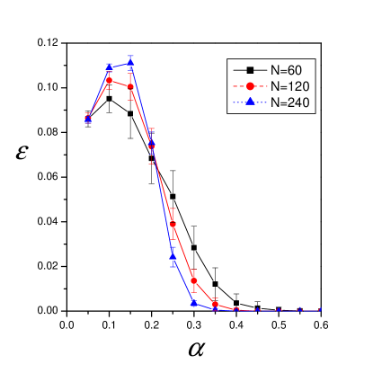
Figure 1: (Color online) Performance. Prediction error $\varepsilon$ as a function of the ratio $\alpha=M/N$ for gene networks with 60 genes (squares), 120 genes (circles) and 240 genes (triangles), averaged over 50 networks. In all cases the performances were obtained using $W_{L1}$ prescription, equal a priori probabilities (i.e. $p_{ij}^{+}=p_{ij}^{-}=p_{ij}^{0}=1/3$ for all $i$ and $j$), $k/N=0.05$ and $a=0.01$.

Figure 1 depicts the prediction error $\varepsilon$ as a function of $\alpha$ defined as the ratio of number experiments and number of genes, i.e. $\alpha=M/N$. These have been tested in three different size networks with $k/N=0.05$, in which all a priori probabilities are assumed to be equals (i.e. $p_{ij}^{+}=p_{ij}^{-}=p_{ij}^{0}=1/3$) and $a=0.01$. For small values of $M$ the method mistakenly infers a percentage of interaction which depends on the network size $N$ and $k$. However, the prediction error decays rapidly as $\alpha$ increases and the gene interaction matrix is completely recovered with a $\alpha$ value that decreases with the network size. This performance was obtained using ${\bf W}_{L1}$ prescription. Similar simulations (data not shown) performed with the ${\bf W}_{L2}$ prescription, reveal that in these cases the prediction error $\varepsilon$ remains close to unit until $\alpha=1$, where they decay abruptly. Dependence of performance on the network topology has not been detected and similar results were obtained for scale free networks which have more biological appeal than the random networks used here. However, these simulations present a greater error bar due to the fact that the network building algorithm used here does not make networks with a uniform node degree.

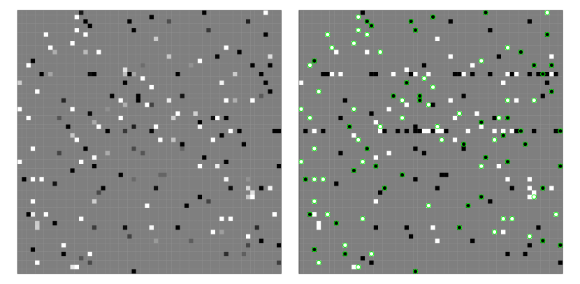
Figure 2: (Color online) Likelihood assessment. Left: connectivity matrix ${\bf W}$ representation related to a random network of 60 genes with $k/N=0.05$. Rows correspond to regulated genes, while columns correspond to the genes acting as regulators. The interaction weights $w_{ij}$ are represented following a linear gray scale, where white corresponds to $w_{ij}=2$, while black to $w_{ij}=-2$. Gray background represents the absence of interaction, i.e. $w_{ij}=0$. Right: gene interaction matrix ${\bf I}$ inferred after 24 random perturbation experiments, using $W_{L1}$ prescription, $a=0.01$ and $p_{ij}^{+}=p_{ij}^{-}=p_{ij}^{0}=1/3$. Circles (green in the online figure) indicate the 94 interactions with an a posteriori probability greater than 0.99. Wrong predictions (35, $\sim 1\%$ of the putative interactions, which in this case) correspond to the regulatory inputs of two genes.

Many times, when dealing with an incomplete data set $M\ll N$, only a percentage of the interactions is inferred correctly. If the likelihood of the inferred paths cannot be assessed, this partial reconstruction has small predictive value in real life. The methodology proposed here can assess the likelihood of the predicted interaction straightforwardly through the a posteriori probability. In this sense, only those predicted interactions with an a posteriori probability which is greater than some significance level can be selected. To illustrate this issue, a network with 60 genes with $k/N=0.05$ was simulated. The related connectivity matrix ${\bf W}$ is represented in Fig. 2(left), row $i$ corresponds to the genes that regulate the activity of gene $i$, while column $j$ corresponds to the genes regulated by gene $j$. The weight values $w_{ij}$ are depicted following a linear gray scale, where white(black) corresponds to the maximum(minimum) values of weights and the gray background represents the absence of interaction. This network is random perturbed in 24 different experiments ($\alpha=0.4$). With this amount of data usually about $\sim 99.5\%$ of the interactions are predicted correctly (see Fig. 1). Nevertheless, which interactions were inferred correctly and which were inferred wrongly is unknown. By mean of the information theory approach, the a posteriori probabilities were computed and the inferred interaction matrix ${\bf I}$ and the associated likelihood were derived. Fig. 2(right) represents the inferred connectivity matrix ${\bf I}$, by assuming that all a priori probabilities are equal (i.e. $p_{ij}^{+}=p_{ij}^{-}=p_{ij}^{0}=1/3$). Red circles indicate wrong predictions ($1\%$ of the interactions), while green circles indicate the interactions with a a posteriori probability greater than 0.99. In this case there are 98(108) interactions where the maximum a posteriori probability is greater 0.99(0.95). A more detailed study (data not show) revealed that interactions related to higher weight values, are associated to high a posteriori probability values. These results suggest that gene networks can be partially recovered even with small amounts of data, mainly for those genes that interact strongly.

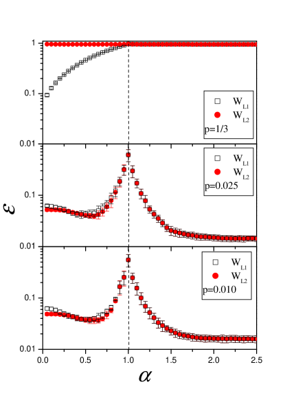
Figure 3: (Color online) Inferring with noisy data. Prediction error $\varepsilon$ as a function of the ratio $\alpha$ for gene networks with 60 genes with $k/N=0.05$. Both input and output data are subject to observational noise of $\eta=0.30$. The performance was obtained using both $W_{L1}$ (open square) and $W_{L2}$ (filled circle) prescriptions and $a=0.01$. Top: the a priori probabilities are equal, i.e. $p_{ij}^{+}=p_{ij}^{-}=p_{ij}^{0}=1/3$ for all $i$ and $j$. Medium: the a priori probabilities are set to be $p_{ij}^{+}=p_{ij}^{-}=0.025$ and $p_{ij}^{0}=0.95$ for all $i$ and $j$. Bottom: the a priori probabilities are set to be $p_{ij}^{+}=p_{ij}^{-}=0.01$ and $p_{ij}^{0}=0.98$ for all $i$ and $j$.

Unfortunately all measurements are subject to observational noise, consequently it is important to asses to what extent the performance of the inference procedure is affected by noise. To simulate this condition in the numerical experiment, the available information $D_{M}$ (both input and output) was corrupted by an additive Gaussian noise with mean zero and standard deviation $\eta$. This inference procedure was performed for networks with $N=60$, in the same condition as for the previous assessment ($p_{ij}^{+}=p_{ij}^{-}=p_{ij}^{0}=1/3$ and $a=0.01$). However, in this case the method based on the prescription of sparseness assumed in $W_{L1}$ could not correctly recovery the gene interaction matrix ${\bf I}$ when the noise level was $\eta=0.3$ (even for smaller $\eta$). Figure 3(top) indicates the prediction error by using both ${\bf W}_{L1}$ and ${\bf W}_{L2}$ assuming that the a priori probability for activation, repression or absence of interaction are equal. This clearly shows that the prediction power decreases as more data becomes available.

However, the network can be partially reconstructed by using an alternative constraint of sparsity. This alternative consists in introducing the knowledge of sparseness of the matrix through the a priori probabilities. That is achieved by setting $p_{ij}^{\pm}\approx 0$ in the inference procedure. Fig. 3(middle) depicts the prediction error as a function of $\alpha$ when the a priori probabilities were set to $p_{ij}^{\pm}=0.025$. The sum of these probability values corresponds to the percentage of genes that are regulated by one gene. With such a priori information, it is possible to reconstruct almost the complete structure of the network (around 95$\%$ of edges) using more experiments than the number of genes, $\alpha\sim 2$. The mean node degree of the network is generally not known in advance. Notwithstanding, the prediction ability is robust for underestimations of the a priori probabilities. Figure 3(bottom) depicts the prediction error as function of $\alpha$ when the a priori probabilities were set to $p_{ij}^{\pm}=0.01$. The result is almost the same as the previous one. This implies that it is possible to partially recover the interaction matrix even with noise data, by setting low values for the a priori probabilities $p_{ij}^{\pm}$. In the last two cases, the prediction performance obtained by the ${\bf W}_{L2}$ prescription is comparable with that obtained by ${\bf W}_{L1}$ using $p_{ij}^{\pm}\approx 0$ prescription, in contrast to the case which deals with clean data. Furthermore, when data are corrupted by noise, it was observed that prediction error has a peak around $\alpha=1$, this peak arises because some singular values, associated to the SVD, take small values as consequence of noise.

The partial recovery referenced above does not pursue recover a closed subnetwork, which mainly infer strong interactions around the whole network. However, in many cases this is crucial to recover the complete subnetwork associated to a given gene or path of interest. The inference approach and information gain tool presented in this study, could be used to establish new relationships between genes and to propose new experiments. By means of cycles of experiments-datamining, the knowledge about the subnetwork can be refined until its complete recovery, even in presence of observational noise. For that purpose the following protocol could be used: i) perform an initial perturbation where the gene of interest is overexpressed, and obtain the genome expression profile; ii) compute the information gain for each gene with this experimental data; iii) select the genes for which the information gain is greater than a given threshold; iv) iterate first two steps perturbing each one of the genes which were selected in the third step and which have still no been perturbed, until no new gene has an information gain greater than the threshold. Figure 4A illustrates the result of three of the experiments-datamining cycles. Firstly, the gene which belongs to the subnetwork of interest, gene g1, is initially overexpressed (level of 10.0 while the other gene levels are random in the range [-0.5,0.5]), then the input-output network is measured, this measurement is subject to observational noise with $\eta=0.30$. The information gain of this experiment is computed for each gene using $p_{ij}^{+}=p_{ij}^{-}=0.01$ as an a priori probability. Subsequently, those genes with $I_{g}$ greater than 1.0 are selected. $I_{g}$ suggests that gene g6 is regulated by g1. Repeating the above step with gene g6, the results indicate that genes g2, g3 are regulated by g6. The above step is repeated with gene g2 and subsequent genes with high information gain values in ensuing experiments, until no new gene with an information gain greater than threshold appears. Fig. 4B illustrates a list of experiments where the first column corresponds to the gene that was perturbed in the experiment, and the second column corresponds to the genes which appear to be regulated by the perturbed gene. In the last two experiments no new regulated genes appeared (which were not indicated in the first column list). The above analysis provides a causal link between two genes, but it does not indicate if the regulation is positive or negative. In order to extract this information, the inference analysis was performed using the ten ”overexpression experiments” pooled in $D_{M}$ ($M=10$). When the inference procedure was applied with this data, 19 out of 24 interactions in the subnetwork were inferred correctly, 10 of them with an posteriori probability greater than 0.99. However, the a priori probabilities provided by the information contained in list of Fig. 4B are included, setting $p_{ij}^{+}=p_{ij}^{-}=0.5$ (or 1/3) for all the pairs $i,j$ indicated in the list, and $p_{ij}^{+}=p_{ij}^{-}=0.01$ otherwise, 23 out of 24 interactions in the subnetwork are inferred, 19 of them with a posteriori probability greater than 0.99, Fig. 4C. The performance above obtained does not differ if the inference procedure is implemented using ${\bf W}_{L2}$ or ${\bf W}_{L1}$ prescription, of course ${\bf W}_{L2}$ is computationally cheaper than ${\bf W}_{L1}$ which requires linear programming optimization.

The above example about subnetwork inference suggests that this novel scheme can be re-used regarding further subnetworks until the whole network is recovered with $M\simeq N$ experiments.

Discussion and Conclusions

A novel approach for regulatory network inference is presented in this study. Differently to other methods, this approach pursues to infer the type of interaction rather than a weight which characterizes the interaction quantitatively. Three main features of the proposed method are pointed out. First, it allows to introduce global a priori information about the network, as sparseness, and other gene dependent available information, as illustrated in the last example Fig. 4C. Second, the information theory formalism provides a way to quantify the likelihood of the inferred paths, by using the a posteriori probabilities computed with the method. Last, but not least, information theory formalism also quantifies the information gained with the set of data to be used in the inference procedure.

Furthermore, the IT approach seems to offer promising perspective as a network inference protocol; the methodology presented here introduces an information gain measure as a bonus. The way in which this quantity could be a useful tool to identify the downstream regulated genes in overexpression experiments is illustrated in this study. This feature allows a datamining-assisted way of uncovering the whole network with a number of experiments equal to the number of genes, even when dealing with a high level of observational noise. This IT approach enables the effective use of all the available information, in which each experiment is used as an individual constraint. Thus, the ensuing observation level becomes much richer than the standard one, where all data define a fitness function to be optimized. Efficient management leads to more realistic results in inference.

The learning protocol presented here constitutes an additional inference technique, which should be of interest not only for basic research but also as an application to many interesting real world problems without paying an excessive computational cost.

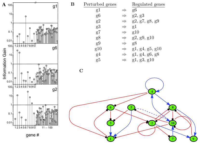
Figure 4: (Color online) Subnetwork identification. A: Information gain $I_{g}$ obtained for three “overexpression experiments”. Firstly, the gene which belongs to the subnetwork of interest, gene g1, is initially overexpressed, then the input-output network is measured, this measurement is subject to observational noise of $\eta=0.30$. The information gain of this experiment is computed for each gene and the genes with $I_{g}$ greater than a given threshold, are selected. $I_{g}$ suggests that gene g6 is regulated by g1. Repeating the above step with gene g6, it appears that genes g2, g3 are regulated by g6. The above step is repeated with gene g2 and subsequent genes with high information gain values in subsequent experiments. B: List of experiments, the first column corresponds to the gene which was overexpressed in each experiment, the second column corresponds to the genes which appear to be regulated by the overexpressed gene. C: Subnetwork inferred 23 out of 24 interactions correctly (solid edges) by this inference procedure using $W_{L2}$ prescription and the above ten ”overexpression experiments” together. The information contained in list B was included as a priori probabilities, i.e., they were set $p_{ij}^{+}=p_{ij}^{-}=0.5$ and $p_{ij}^{0}=0.0$ for all $i,j$ pairs indicated in the list, and $p_{ij}^{+}=p_{ij}^{-}=0.01$ otherwise.

References

- (1) Ideker T, Galitski T, Hood L (2001) A new approach to decoding life: systems biology. Annu Rev Genomics Hum Genet 2:343–372.
- (2) Tienda-Luna IM, Yin Y, Carrion MC, Huang Y, Cai H, Sanchez M, Wang Y (2008) Inferring the skeleton cell cycle regulatory network of malaria parasite using comparative genomic and variational Bayesian approaches. Genetica 132:131–142.
- (3) Gardner TS, Di Bernardo D, Lorenz D, Collins JJ (2003) Inferring genetic networks and identifying compound mode of action via expression profiling. Science 301:102- 105.
- (4) Tegnér J, and Björkegren J (2007) Perturbations to uncover gene networks. Trends in Genetics 23:34–41.
- (5) Holter NS, Maritan A, Cieplak M, Fedoroff NV, Banavar JR (2001) Dynamic modeling of gene expression data. Proc. Natl. Acad. Sci. USA 98:1693 -1698.
- (6) Tegnér J, Yeung MK, Hasty J, Collins JJ (2003) Reverse engineering gene networks: integrating genetic perturbations with dynamical modeling. Proc. Natl. Acad. Sci. USA 100:5944- 5949.
- (7) Pe´Er D, Regev A, Elidan G, Friedman N (2001). Inferring subnetworks from perturbed expression profiles. Bioinformatics 17:S215 -S224.
- (8) Husmeier D (2003) Sensitivity and specificity of inferring genetic regulatory interactions from microarray experiments with dynamic Bayesian networks. Bioinformatics 19:2270- 2282.
- (9) Beal MJ, Falciani F, Ghahramani Z, Rangel C, Wild DL (2005) A Bayesian approach to reconstructing genetic regulatory networks with hidden factors. Bioinformatics 21:349 -356.
- (10) Akutsu T, Miyano S, Kuhara S (2000) Inferring qualitative relations in genetic networks an metabolic pathways. Bioinformatics 16:727-734.
- (11) D´Haeseleer P, Liang S, Somogyi R (2000) Genetic network inference: from co-expression clustering to reverse engineering. Bioinformatics 16:707–726.
- (12) D´Haeseleer P, Wen X, Fuhrman S, Somogyi R (1999) Linear modeling of MMA expression levels during CNS development and injury. Pac. Symp. Biocomput 41- 52.
- (13) van Someren EP, Wessels LFA, Backer E, Reinders MJT (2002) Genetic network modeling. Pharmacogenomics 3:507–525.
- (14) Shannon CE and Weaver W (1949) The Mathematical Theory of Communication (University of Illinois Press, Chicago).
- (15) Jaynes ET (1957) Phys Rev 108:171–190.
- (16) Lezon T, Banavar J, Cieplak M, Maritan A, and Fedoroff NV (2006) Using the principle of entropy maximization to infer genetic interaction networks from gene expression patterns. Proc. Natl. Acad. Sci. USA 103:19033- 19038.
- (17) Martínez O, Reyes-Valdés MH (2008) Defining diversity, specialization, and gene specificity in transcriptomes through information theory Proc. Natl. Acad. Sci. USA 105:9709–9714.
- (18) Wang Y, Joshi T, Zhang X-S, Xu D, Chen L (2006) Inferring gene regulatory networks from multiple microarray datasets. Bioinformatics 22:2413–2420.
- (19) Yeung MK, Tegner J, Collins JJ (2002) Reverse engineering gene networks using singular value decomposition and robust regression. Proc. Natl. Acad. Sci. USA 99:6163- 6168.
- (20) Levine RD, Tribus M (1978) The Maximum Entropy Principle (MIT Press, Boston MA).