Multifractal Detrended Cross-Correlation Analysis of Sunspot Numbers and River Flow Fluctuations

Abstract

We use the Detrended Cross-Correlation Analysis (DCCA) to investigate the influence of sun activity represented by sunspot numbers on one of the climate indicators, specifically rivers, represented by river flow fluctuation for Daugava, Holston, Nolichucky and French Broad rivers. The Multifractal Detrended Cross-Correlation Analysis (MF-DXA) shows that there exist some crossovers in the cross-correlation fluctuation function versus time scale of the river flow and sunspot series. One of these crossovers corresponds to the well-known cycle of solar activity demonstrating a universal property of the mentioned rivers. The scaling exponent given by DCCA for original series at intermediate time scale, $(12-24)\leq s\leq 130$ months, is $\lambda=1.17\pm 0.04$ which is almost similar for all underlying rivers at $1\sigma$confidence interval showing the second universal behavior of river runoffs. To remove the sinusoidal trends embedded in data sets, we apply the Singular Value Decomposition (SVD) method. Our results show that there exists a long-range cross-correlation between the sunspot numbers and the underlying streamflow records. The magnitude of the scaling exponent and the corresponding cross-correlation exponent are $\lambda\in(0.76,0.85)$ and $\gamma_{\times}\in(0.30,0.48)$, respectively. Different values for scaling and cross-correlation exponents may be related to local and external factors such as topography, drainage network morphology, human activity and so on. Multifractal cross-correlation analysis demonstrates that all underlying fluctuations have almost weak multifractal nature which is also a universal property for data series. In addition the empirical relation between scaling exponent derived by DCCA and Detrended Fluctuation Analysis (DFA), $\lambda\approx(h_{\rm sun}+h_{\rm river})/2$ is confirmed.

]

I Introduction

Recently, due to the developments in the area of complex systems as well as data measurements and data analysis, one can find many opportunities for examination and interpretation of climate change which exhibit irregular systems [1, 2, 3, 4, 5, 6, 7, 8]. It is well shown that the climate system is enforced by the well-defined seasonal periodicity, however the existence of unpredictable perturbation and chaotic functioning lead to extreme climate events. Indeed the climate is a dynamical system affected by tremendous factors and variables, such as solar activity which is represented by Sunspot numbers in this research [4, 5, 6, 7, 8, 9, 10]. All factors that control the trajectory of such mentioned systems have enormously large phase space and evolve as non-stationary processes, consequently we should explore it with stochastic tools to achieve reliable results. Nowadays, it has been clarified that a remarkably wide variety of natural systems can be characterized by long-rangeSuch cross-correlations address scientists toward fractal geometry of the underlying dynamical systems and can hopefully help us to predict future events. Existence and determination of power-law cross-correlations would help to promote our understanding of the corresponding dynamics and their future evolutions [11, 12, 13, 14]. Beside, many events which controls earths climate, water runoff records assigned by rivers and sun activity play a crucial and survival roles for human life. The runoff water fluctuations are excellent climate criteria because they integrate evapotranspiration (output) and precipitations (input) over large areas. It is well accepted that the prediction of water runoff is fundamental for different aspects of social and economical reasons, ranging from the prediction of floods and droughts to planning of agricultural conditions. As a result of the periodicity in precipitation, river flow has also strong seasonal periodicity [12]. It is worth to note that unlike other climate components, water runoff may be directly influenced by human activity, like agriculture, drainage network morphology and so on, consequently makes it hard to distinguish the artificial and natural effects on the river flow data. Finding some or at least a universal behavior for different streamflow fluctuations as well as quantifying the impact of sun activity on various temporal and spatial scales of water runoff fluctuations can improve the recent hydrological models [15].

To this end, the statistical and multifractal analysis of river flows as well as influence of sun activity due to the interior and exterior chemical and physical properties of sun should be an important issue in the geophysical and hydrological systems.

The streamflow of rivers and sun activity have been studied from various point of views such as: the probability distribution [16, 17], correlation and fractal behaviors [18, 19, 20, 21, 22, 23], connection between volatility and nonlinearity of fluctuations [11, 12, 24, 25], scale invariance for distribution function [26]. In addition, sun activity have been investigated by some methods in chaos theory [27] and also multifractal analysis [28, 29], wavelet analysis [30], cross-correlation functions between monthly mean sunspot areas and sunspot numbers [31, 32], the relation between sunspot numbers fluctuation and number of flares, their evolution step [33, 34], principal components and neural network methods to predict sunspots [35, 36], sunspot areas time series and solar irradiance reconstructions [37], magnetic and dynamic properties of sunspots at the photospheric level [38] and the hydraulic-geometric similarity of river [39, 40, 41].

More recently, Pablo J. D. Mauas et. al., have investigated the solar forcing on climate, using the quantification of cross-correlation between the yearly sunspot numbers, irradiance reconstruction and streamflow of Paraná river [9, 10]. On the other hand, the mechanisms for solar influence on the earth’s climate has been clarified in detailed from various point of views in [42]. Q. Zhang et. al., have investigated the universal behavior of streamflow records of the Pearl river [15].

After innovation of Hurst to propose the self-similar processes and its criteria, namely “Hurst exponent” [18, 19, 20, 21, 22, 23], long-range correlated fluctuation behavior has also been reported for vast category of sciences, specifically the geophysical records (for more discussion see [18, 19, 20, 21, 22, 23, 43, 44, 45, 46]). In the last decade, the modification prescription which is required for a full characterization of many data sets such as the runoff records, the various moments of the so-called fluctuation functions, have been introduced [18, 19, 20, 21, 22, 23]. The effect of non-stationarity on the detrended fluctuation analysis has been investigated in [47, 48].

Here we take a new approach and rely on the state-of-the-art algorithm to investigate the contribution of sinusoidal trends embedded in the data set as well as non-stationarity properties of the underlying series. We implement robust methods to explore the multifractal nature of cross-correlation between two important climate variables, the monthly streamflow of some rivers and sun activity represented by sunspot numbers (see Figure (1)), by using the novel approach in the fractal analysis, Detrended Cross-Correlation Analysis (DCCA) and its multifractal modification, the Multifractal detrended Cross-Correlation Analysis (MF-DXA) [49, 50]. We restrict this article to use the sunspot numbers as the solar activity indicator, since there are many large and reliable data sets which can be considered as solar influence on the climate. Due to the presence of the sinusoidal trends in both sunspot numbers and the runoff river fluctuations and based on previous researches, one cannot expect to find a unique scaling behavior for fluctuation functions in all time scales (see section III), consequently, we have been motivated to use the well-known method, namely Singular Value Decomposition (SVD) method to exclude dominant trends in data set (see section II for more details). So after, clean data set will be used in the DCCA and MF-DXA methods.

This paper is organized as follows: in section II, we describe the methods which are used to determine the cross-correlation of two non-stationary time series, the Detrended Cross-Correlation Analysis (DCCA), and investigate the corresponding multifractal properties by us- ing the Multifractal Detrended Cross-Correlation Analysis (MF-DXA). Section II will be continued by introducing a method to eliminate trends from the original data set, the Singular Value Decomposition (SVD), and describing data used in this paper. In section III, the multifractal cross-correlation of the underlying data sets will be examined. Section IV, will be devoted to the results and summary.

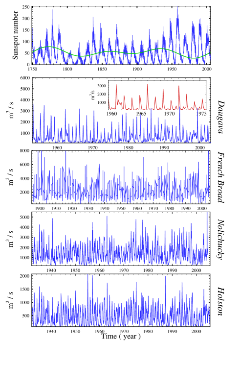
FIG. 1.: Upper panel corresponds to the monthly sunspot number data set. The secular trend, obtained with a low-pass Fourier filter is shown as a thick line in the upper panel. Lower panels indicate observed flux fluctuations of Daugava, French Broad, Nolichucky and Holston rivers, respectively. The inset plot shows river flow for small scales.

II Analysis techniques AND data description

Time series measured in the nature are usually affected by non-stationarities such as trends and artificial noises which must be well distinguished from the intrinsic fluctuations of the series. In many cases also, intrinsic fluctuations behave as non-stationary processes. Consequently, common methods in data analysis will be encountered with spurious or at least unreliable results. One of the most famous and well-known approach used in many studies is Multifractal Detrended Fluctuations Analysis (MF-DFA) [51, 52]. This method has been applied to various areas, such as economical time series [53, 54, 55, economics-3, 56], river flow [13] and sunspot fluctuations [57, 58], cosmic microwave background radiations [59], music [60, 61], plasma fluctuations [62].

For many reasons, we are interested in studying the mutual influence of two series in the presence of non-stationarities. Obviously, traditional methods for this investigation become inaccurate procedures. Recently Jun et. al. have proposed an approach for analyzing correlation properties of a series by decomposing the original signal into its positive and negative fluctuation components [63]. Based on the previous study, Podobnik et. al. have modified the mentioned correlation method and improved it to explore the cross-correlation between two non-stationary fluctuations, named Detrended Cross-Correlation Analysis (DCCA) [49] and its generalized, the Multifractal Detrended Cross-Correlation Analysis (MF-DXA) which also examine higher orders detrended covariance[50].

As mentioned before, trends in data set may influence the accuracy of results. For reliable detection of the cross-correlations, it is essential to distinguish trends from the intrinsic fluctuations in data. Generally, trends embedded in measurements are of two types: Polynomial and Sinusoidal trends. Although the MF-DFA and MF-DXA methods eliminate the polynomial trends, the sinusoidal trends remain [47, 48]. There are several robust methods to eliminate the sinusoidal one such as Fourier Detrended Fluctuations Analysis (F-DFA) [62, 64], which is actually a high-pass filter, and Singular Value Decomposition (SVD) [65, 66]. One of the most disadvantage of the F-DFA method is the reduction of the size of underlying data set. To apply the MF-DXA (see the following subsection), we have to synchronize two underlying data set which may not be done using the F-DFA method. On the other hand, the SVD method promises to remain the length as well as synchronization [65, 66]. Here in order to eliminate the effect of sinusoidal trends, we apply the Singular Value Decomposition (SVD) [65, 66]. After trends elimination, we use the MF-DXA to analyze the cleaned data sets.

A DCCA and MF-DXA

One of the newly methods in analyzing two non-stationary time series is Detrended Cross-Correlation Analysis (DCCA)[49, 63]. This method is a generalization of the DFA method in which only one time series was analyzed. Recently a generalized version of the DCCA method which is so-called MF-DXA, has been introduced [50]. Just same as the MF-DFA method, MF-DXA consists of the $4$ steps (see [49, 50, 67] for more details):
(I): Computing the profiles of the underlying data series, $x_{k}$ and $y_{k}$, as

$$X(i) \equiv \sum_{k=1}^{i}\left[x_{k}-\langle x\rangle\right]\qquad i=1,\ldots,N$$ (1)

$$Y(i) \equiv \sum_{k=1}^{i}\left[y_{k}-\langle y\rangle\right]\qquad i=1,\ldots,N$$ (2)

the subtraction of mean is not compulsory. Since we are going to compare two different time series, we construct data sets with zero mean and unit variance using initial ones.

(II): Dividing each of the profile into $N_{s}\equiv{\rm int}(N/s)$ non-overlapping segments of equal lengths $s$, and then computing the fluctuation function for each segments. In order to take the whole series into account when the size of the data sets is not a multiple of considered time scale, $s$, we do the same procedure from the opposite end, consequently one finds $2N_{s}$ segments.

$$F(s,m)={1\over s}\sum_{i=1}^{s}\{Y[(m-1)s+i]-y_{m}(i)\}$$ (3)

$$\qquad\qquad\qquad\qquad\times\{X[(m-1)s+i]-x_{m}(i)\}$$ (4)

for $m=1,...,N_{s}$ and:

$$F(s,m)={1\over s}\sum_{i=1}^{s}\{Y[N-(m-1)s+i]-y_{m}(i)\}$$ (5)

$$\qquad\qquad\qquad\qquad\times\{X[N-(m-1)s+i]-x_{m}(i)\}$$ (6)

for $m=N_{s}+1,...,2N_{s}$, where $x_{m}(i)$ and $y_{m}(i)$ are a fitting polynomial in segment $m$th. Usually, a linear function is selected for fitting the function. If there is no trend in the data, a zeroth-order fitting function might be enough [68].

(III): Averaging the local fluctuation function over all the part, given by:

$$F_{q}(s)=\left\{{1\over N_{s}}\sum_{m=1}^{N_{s}}\left[F(s,m)\right]^{q/2}\right\}^{1/q}$$ (7)

Generally, $q$ can take any real value, except zero. For $q=0$, equation (7) becomes:

$$F_{0}(s)=\exp\left({1\over 2N_{s}}\sum_{m=1}^{N_{s}}\ln F(s,m)\right)$$ (8)

For $q=2$, the standard DCCA is retrieved.

(IV): The final step is calculating the slope of the log-log plot of $F_{q}(s)$ versus $s$ which directly determines the scaling exponent $\lambda(q)$, as:

$$F_{q}(s)\sim s^{\lambda(q)}$$ (9)

If both underlying series are equal then $\lambda(q)$ is nothing else but so-called generalized Hurst exponent, $h(q)$. In the absence of sinusoidal trends embedded in data sets, if one finds no scaling behavior for the fluctuation function in equation (9) or at least, there does not exist any unique exponent for all scaling ranges then there exists either short-range cross-correlation or not at all any cross-correlation. For a series of size $N$, the minimum number of windows will be $N_{s}=2$ corresponding to the maximum value of $s={\rm int}(N/2)$. In addition, it has been demonstrated that to find the most correct value of scaling exponent by using DFA and DCCA methods, we should set $s\leq(N/2)$, namely $N_{s}\geq 2$ [52].

To determine the slope of curve in the log-log plot of fluctuation function versus scale (equation (9)), we use Bayesian statistics[69] . We introduce measurements and model parameters as $\{X\}:\{F_{q}(s)\}$ and $\{\Theta\}:\{\lambda(q)\}$, respectively. Based on the Bayesian theorem, the conditional probability of the model parameters given data set (observation) is so-called posterior probability and is given by:

$$P(\lambda(q)|X)=\frac{{\mathcal{L}}(X|\lambda(q))P(\lambda(q))}{\int{\mathcal{L}}(X|\lambda(q))d\lambda(q)}$$ (10)

where the first term in the nominator of the right hand side is Likelihood and the second term contains all initial constraints concerning model parameters, so-called prior distribution. This term expresses the degree of belief about the model. In the absence of every prior constraints, the posterior function, $P(\lambda(q)|X)$ is proportional to the Likelihood function. If there is no correlation between various measurements, consequently according to the central limit theorem, Likelihood function is given by a product of Gaussian functions as follows:

$${\mathcal{L}}(X|\lambda(q))\sim\exp\left(\frac{-\chi^{2}(\lambda(q))}{2}\right)$$ (11)

where:

$$\chi^{2}(\lambda(q))=\int ds\frac{[F_{{\rm obs.}}(s)-F_{{\rm The.}}(s;\lambda(q))]^{2}}{\sigma_{{\rm obs.}}^{2}(s)}$$ (12)

Here $F_{{\rm obs.}}(s)$ and $F_{{\rm The.}}(s;\lambda)$ are fluctuation function computed directly from the data set by using DFA or DCCA and determined by equation (6), respectively. Also, $\sigma_{{\rm obs.}}(s)$ is the mean standard deviation, associated to $F_{\rm obs.}(s)$. Apparently, this Likelihood function to be maximum when for a value of the scaling exponent, $\lambda(q)$, $\chi^{2}$ reaches to its global minimum. The value of error-bar at $1\sigma$ confidence interval of $\lambda(q)$ is determined by the likelihood function based on the following condition:

$$68.3\%=\int_{-\sigma^{-}}^{+\sigma^{+}}{\mathcal{L}}(X|\lambda(q))d\lambda(q)$$ (13)

Finally we report the best value of scaling exponent at $1\sigma$ confidence interval according to $\lambda_{-\sigma^{-}}^{+\sigma^{+}}$ for each moment, $q$’s.

B Singular Value Decomposition (SVD)

Determining trends and construction proper detrending operations are important step toward robust analysis, specially in climatic data analysis. As given by Z. Wu and his collaborators [70], there is no unique definition of trend and any proper algorithm for extracting it from underlying stationary as well as non-stationary data sets. In another aspect, the trend in a real world data series, non-stationary one, is an intrinsic function imposed by the nature on data set. To identify the trend on a data set, we can investigate the series in whole domain or on some specific span of domains. For linear and stationary data sets choosing the length of data set as domain of trend may be suit but for a real world data set which is non-stationary and nonlinear, we need more precise definition of trend. As of the importance of investigating trends and probably removing them from series, one can point out to two following aims:
I) In some cases, there exists one or more crossover (time) scales, $s_{\times}$, in the log-log plot of $F_{q}(s)$ versus $s$ (equation (9)), segregating regimes with different scaling exponents. These patterns demonstrates that underlying fluctuation has different correlation behavior in various values of scales [47, 48, 65, 66, 71].
II) In many cases, crossovers are produced by the embedded sinusoidal trends, e.g. seasonal trends in the climate time series. Subsequently, to find scaling exponent of the intrinsic fluctuations, we should remove sinusoidal trends by using most robust detrending method so after, produced clean data set is used as an input for DCCA and MF-DXA methods [47, 48, 62].

In order to remove trends corresponding to the low frequency periodic behavior, we use Singular Value Decomposition method [72] instead of transformation a recorded data to the Fourier space using the method proposed in [73] (see also [47, 48, 71]). Using the SVD method not only we can track the influence of sinusoidal trends on the results, but also the synchronization of two underlying data sets will be guaranteed [65, 66]. In addition, we can determine over which scale, noises or trends have dominant contribution also the value of so-called crossover in the fluctuation function, in terms of the scale is computed by using DCCA method. [64, 65, 66, 74, 75]. After removing the dominant periodic functions, such as sinusoidal trends, we obtain the fluctuation exponent by direct application of the MF-DXA.
The SVD method consists of the following steps:

(I): Consider a data set which is superimposed with periodic trends $\{x_{i}\};i=1,...,N$. Embed $x_{i}$ with parameters $(d,\tau)$ where $d$ and $\tau$ are the embedding dimension and the time delay, respectively. The embedded data can be represented as a matrix $\mathbf{\Gamma}$ given by:

$$\mathbf{\Gamma}\equiv\left(\begin{array}[]{cccc}x_{1}&x_{1+\tau}&...&x_{1+N-(d-1)\tau-1}\\ \vdots&\vdots&\vdots&\vdots\\ x_{i}&x_{i+\tau}&...&x_{i+N-(d-1)\tau-1}\\ \vdots&\vdots&\vdots&\vdots\\ x_{d}&x_{d+\tau}&...&x_{d+N-(d-1)\tau-1}\\ \end{array}\right)$$ (14)

as one can see, $1\leq i\leq d$. For a periodic embedded trend, we set $p$ as the number of dominant frequency components of the form $e^{({\rm i}\omega_{k}t)}$, $k=1...p$ in their power spectrum. For a fixed value of sample size, $N$, the maximum value of $d$ in the so-called trajectory matrix, $\mathbf{\Gamma}$, equates to $d\leq N-(d-1)\tau+1$ [66, 74, 76].

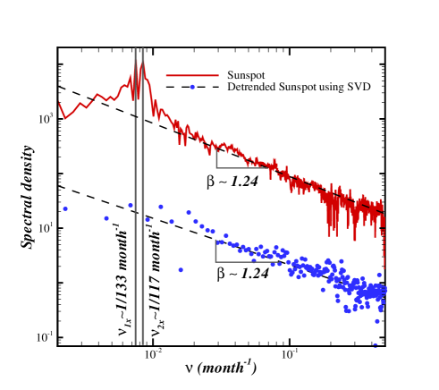
FIG. 2.: Power spectrum of the original sunspot numbers data set (solid line) and that of for a cleaned one using SVD method (filled symbols). Dashed lines correspond to the scaling function as $\nu^{-\beta}$ for the same signals without sinusoidal trends.

(II): Matrix $\mathbf{\Gamma}$ will be decomposed to the two left and right orthogonal matrices as follows:

$$\mathbf{\Gamma}={\mathbf{USV^{\dagger}}}$$ (15)

where ${\mathbf{U}}_{d\times d}$ and ${\mathbf{V}}_{(N-(d-1)\tau)\times(N-(d-1)\tau)}$ are the left and right orthogonal matrices, respectively. The diagonal elements of ${\mathbf{S}}_{d\times(N-(d-1)\tau)}$ are the desired singular values, also known as eigenvalues. The Singular Value Decomposition of $\mathbf{\Gamma}$ is related to the eigendecomposition of the symmetric matrices $\mathbf{\Gamma}^{\dagger}\mathbf{\Gamma}$ and $\mathbf{\Gamma}{\mathbf{\Gamma}}^{\dagger}$, as ${\mathbf{\Gamma^{\dagger}\Gamma v_{i}}}=\lambda_{i}^{2}\mathbf{v_{i}}$ and ${\mathbf{\Gamma\Gamma^{\dagger}u_{i}}}=\lambda_{i}^{2}\mathbf{u_{i}}$. The nonzero eigenvalues of $\mathbf{\Gamma^{\dagger}\Gamma}$ are the same as that of $\mathbf{\Gamma\Gamma^{\dagger}}$; and determine the rank of $\mathbf{\Gamma}$. The eigenvalues are ordered such that $\lambda_{i}>\lambda_{i+1}\geq 0$. The diagonal elements of $\mathbf{S}$ will be constructed by the ordered eigenvalues (the others will be set to zero). The rank of $\mathbf{\Gamma}$ is equal to the number of nonzero eigenvalues. The columns of $\mathbf{U}$ and $\mathbf{V}$ are constructed by the $\mathbf{u_{i}}$ and $\mathbf{v_{i}}$, namely the eigenvectors mentioned before, corresponding to the ordered eigenvalues.

By applying the SVD to the matrix $\mathbf{\Gamma}$ (i.e., $\mathbf{\Gamma}=USV^{\dagger}$) we will get $\mathbf{U}$, $\mathbf{S}$ and $\mathbf{V}$. We consider the number of frequency components in the periodic trend to be $p$. Set the dominant $2p+1$ eigenvalues in the matrix $\mathbf{S}$ to zero and hereafter named as $\mathbf{S^{*}}$. The filtered matrix ${\mathbf{\Gamma}^{*}}_{d\times(N-(d-1)\tau)}$ determined by $\mathbf{\Gamma}^{*}=US^{*}V^{\dagger}$ with elements $\Gamma^{*}_{ij}$. This in turn is mapped back on to a one-dimensional or filtered data given by:

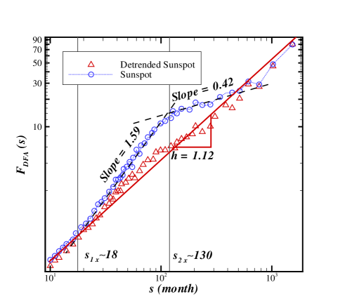
FIG. 3.: The DFA results of the original sunspot number data set and filtered one using SVD. The solid line corresponds to power fit of fluctuation. The slope of power fits has been calculated by likelihood analysis (see the text).

$$x^{*}_{i+j-1}=\Gamma^{*}_{ij}$$ (16)

where $1\leq i\leq d$ and $1\leq j\leq N-(d-1)\tau$. The $p$ dominant eigen-values and associating eigendecomposed vectors, represent trends subspace subsequently, the remaining $(d-p)$ eigenvalues and corresponding eigenvectors demonstrate intrinsic fluctuations subspace. In order to determine the value of $p$ for a typical series such as monthly sunspot data set, at first, we compute the power spectrum of monthly sunspot numbers. As shown in Figure (2), there are at least two dominant sinusoidal trends embedded in the monthly sunspot numbers. The first one corresponds to the well-known sun activity and second period belongs to the so-called Schwabe cycle interval. In order to eliminate mentioned trends, we set $p=2$ in the SVD algorithm and compute the power spectrum of the cleaned data again. Our expectation is that there must be no deviation from scaling function as $\nu^{-\beta}$ with $\beta=2h(q=2)-1=1.24\pm 0.02$ as one can see in the lower plot in Figure (2). It is worth to note that by increasing $p$ from its optimum value in the SVD method, probably some intrinsic statistical properties of underlying data set will be destroyed. After which we use the detrended sunspot series as an input data for common DFA method (see Figure (3)). As shown in Figure (3), all of the crossover time scales which are produced due to the competition between sinusoidal trends embedded in sunspot series and intrinsic fluctuations, were diminished and intrinsic fluctuations will be retrieved. Our result is in agreement with the previous result regarding to scaling behavior of sunspot based on MF-DFA method accompanying by Fourier-Detrended Analysis, reported in [57]. Figure (3) confirms that, SVD method could remove sinusoidal trends.

In the log-log plot of fluctuation function versus time scale given by DFA method, also one can find three crossovers (see Figure (3)). To determine their value, we define error function as:

$$\Delta(s)=\sqrt{\left[F_{\rm obs.}(s)-F_{\rm{Linear}}(s)\right]^{2}}$$ (17)

for each $q$, where $F_{\rm obs.}(s)$ and $F_{\rm{Linear}}(s)$ are the fluctuation functions for the original data and the filtered data produced by the SVD method, respectively. In Figure (4) we plot $\Delta$ as a function of $s$ for the sunspot numbers fluctuations. The first crossovers occurs at $s_{1\times}\sim[12-18]$ months corresponding to the annual period. The second crossovers is equal to $s_{2\times}\sim[130-170]$ months which is related to the well-known solar activity period. We cannot determine the value of third crossover with the acceptable uncertainty by using DFA method due to small size of current sunspot series.

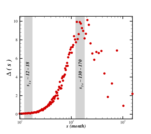
FIG. 4.: $\Delta$ function versus time scale.

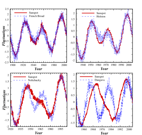
FIG. 5.: The detrended fluctuations of rivers (dashed line) and the corresponding sunspot (solid line) time series. Here we use a SVD method to trend series. The mean and variance of each series became zero and unity, respectively. The Pearson’s correlation coefficients are $r_{\rm Daugava}=+0.44$, $r_{\rm Holston}=+0.94$, $r_{\rm Nolichucky}=+0.88$ and $r_{\rm FrenchBroad}=+0.94$.

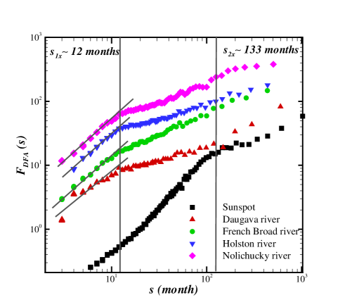
FIG. 6.: Fluctuation function versus scale in log-log plot computed by DFA method for original data sets. To make more sense we shifted the vertical scale.

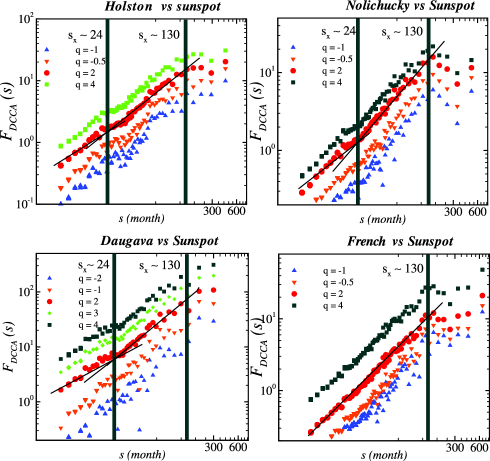
FIG. 7.: Log-log plot of fluctuation functions given by the MF-DXA ($F_{DCCA}(s)$) method for various values of $q$ for four rivers’ flow mentioned in the manuscript versus sunspot numbers as a function of time scale. Here $s_{max}=[{\rm size}\quad{\rm of}\quad{\rm series}/2]$. We shifted the vertical scale to make more sense.

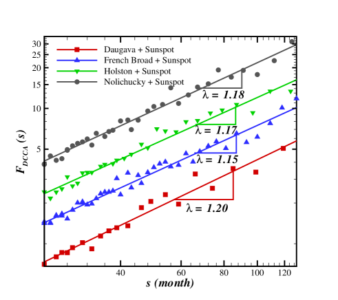
FIG. 8.: Log-log plot of fluctuation functions given by DCCA($F_{DCCA}(s)$) method for four streamflows fluctuations versus sunspot numbers as a function $s$ at intermediate time scale, $12-24\leq s\leq 130$ months. For clearly, we shifted the vertical scale. Solid lines correspond to the power fit of fluctuation function and slopes have been computed by likelihood analysis.

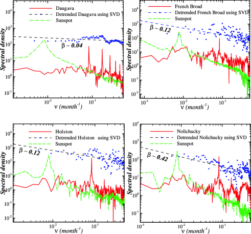
FIG. 9.: Spectral density of river flow fluctuations, detrended data set and synchronizing sunspot numbers. We shifted the vertical scale for spectral density to make more sense.

C Data Description

We use the up-to-date monthly sunspot numbers ($S_{N}$) data series released by National Oceanic and Atmospheric Administration (NOAA) [77] and the Sunspot Index Data Center (SIDC) [78]. The monthly flow fluctuations of four famous rivers, namely Daugava at Latvia, Holston near Damascus, Nolichucky at Embreeville and French Broad at Asheville were collected from National Water Information System [79]. The original Daugava river data source is Latvian Environmental Geological and Meteorological Agency database [80]. The runoff dimension of the underlying rivers is m³/s (see Figure (1)). The river flow fluctuations have been measured independently in corresponding area. All mentioned rivers are mixed feeding from rain, snowmelt water and groundwater. Table (I) reports some characteristics of river flow fluctuations used in this study. These data sets are almost long in length and most available series. In Figure (5) we plot underlying streamflows and sunspot numbers detrended data sets. In this figure, we use SVD method explained in the previous subsection for detrending data sets, also the mean and variance of series equate to zero and unity, respectively. According to Figure (5), one may find a remarkable correlation for streamflows and sunspot numbers. To quantify this correlation we use the Pearson’s correlation coefficients for ${X}$ and ${Y}$ defined by: $r=\frac{\langle X-\langle X\rangle\rangle\langle Y-\langle Y\rangle\rangle}{\sqrt{\langle X-\langle X\rangle\rangle\langle Y-\langle Y\rangle\rangle}}$. The value of $r$ for detrended river flows and sunspot numbers correspond to $r_{\rm Daugava}=+0.44$, $r_{\rm Holston}=+0.94$, $r_{\rm Nolichucky}=+0.88$ and $r_{\rm French-Broad}=+0.94$.

TABLE I.: The main characteristics of runoff rivers used in this paper.

River	Discharge	Series Length	Drainage	Location
	(m${}^{3}/$sec)		area(km2)
French Broad	$2093$	$1896.1-2005.12$	2448	$35^{\circ}36^{\prime}$ N
				$82^{\circ}34^{\prime}$ W
Daugava	$601$	$1953.1-2002.12$	87900	$56^{\circ}57^{\prime}$ N
				$24^{\circ}6^{\prime}$ E
Holston	$479$	$1931.1-2005.12$	784.8	$36^{\circ}39^{\prime}$ N
				$81^{\circ}50^{\prime}$ W
Nolichucky	$1379$	$1921.1-2005.12$	2085	$36^{\circ}10^{\prime}$ N
				$82^{\circ}27^{\prime}$ W

III MF-DXA of Sunspots and River flow fluctuations

To examine the multifractal properties and cross-correlation of sunspot numbers and river flow fluctuations, we apply the DCCA and MF-DXA methods. As mentioned in the previous section, we have to synchronize two time series of interests. The length of the river flow fluctuations may vary from 600 to 1300 months for the studied rivers, Daugava, Nolichucky, Holston and French Broad. On the contrary, there is more information available for sunspot databases, ranging from daily to annually data sets. To find reliable results given by DCCA, we synchronized the sunspot monthly series to all four river’s data sets.

Before applying any detrending program we apply DFA, DCCA and MF-DXA method. Log-log plot of $F(s)$ versus $s$ for original streamflow and sunspot data sets by using DFA method (Figure (6)) confirms that all underlying runoff rivers behave as the anti-persistent long-range correlated series for time scale $s<12$ months. the value of Hurst exponent at this scale for Daugava, Holston, Nolichucky, French Broad and sunspot correspond to $H_{\rm Daugava}=h(2)-1=0.21\pm 0.02$, $H_{\rm Holston}=h(2)-1=0.22\pm 0.02$, $H_{\rm Nolichucky}=h(2)-1=0.21\pm 0.02$, $H_{\rm French-Broad}=h(2)-1=0.18\pm 0.03$ and $H_{\rm Sunspot}=h(2)-1=0.11\pm 0.03$, respectively.

Figure (7) shows the fluctuation function given by multifractal DCCA method for each river flow fluctuations versus sunspot numbers without applying any detrending procedure. Some crossover time scales in fluctuation functions are detected in Figure (7). One of those crossovers is known as cycle of solar activity. In addition the scaling behavior of fluctuation function at intermediate time scales, namely $[12-24]\leq s\leq 130$ months, is similar at $1\sigma$ confidence interval for $q=2$ for all rivers used in this paper (see Figure (8)). The scaling exponent at this regime is $\lambda(q=2)=1.17\pm 0.04$. As shown in Ref. [48], trends become dominant at intermediate regimen while at small and very large time scales, the intrinsic fluctuations to be dominated, therefor, we conclude that at $[12-24]\leq s\leq 130$ months the cross-correlation of water runoff and corresponding sunspot numbers determined by DCCA method for $q=2$, is characterized as the universal behavior. For $s<[12-24]$ and $s>130$ months the slopes of fluctuation functions are different for various rivers and implies that at mentioned time scales the local effects such as morphology, human activities, various drainage areas become dominant [15, 81]. Moreover, cycle of solar activity represented by sunspot is one of most robust effect which affects on streamflow fluctuations.

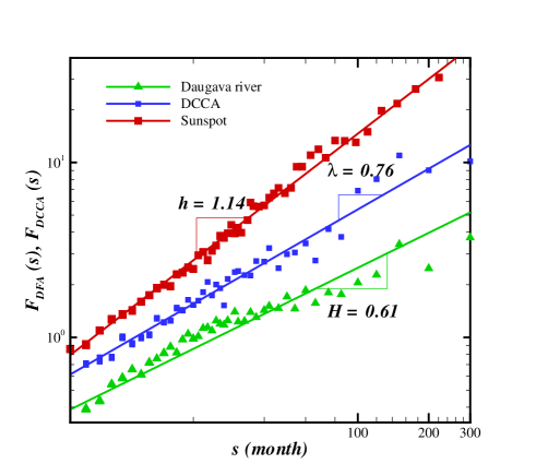
FIG. 10.: Log-log plot of fluctuation functions given by DFA ($F_{DFA}(s)$) and DCCA ($F_{DCCA}(s)$) methods for detrended sunspot numbers and Daugava river flow as a function of time scale. Where we choose $q=2$. The slope of power fits have been derived by likelihood statistics.

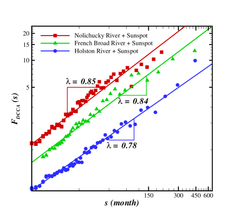
FIG. 11.: Fluctuation function given by DCCA method for detrended Holston, French Broad and Nolichucky rivers with their synchronized sunspot series in log-log scale versus time for $q=2$. The maximum value of $s$ for each series equates to the integer part of half size of the corresponding river flow.

Figure (9) shows the power spectrum of original and detrended mentioned rivers data sets and synchronized sunspot numbers series. The spectral density of French Broad and Nolichucky rivers behave in similar way around the well-known solar activity. This outcome is also confirmed in Figure (7), since there is a sharp crossover in the fluctuation function versus $s$, in the MF-DXA method for French Broad and Nolichucky rivers. This may demonstrate that the contribution of solar activity depends on the geographical properties of river.

Now, to explore the existence of cross-correlation in data set without sinusoidal trends from the DCCA and MF-DXA method we detrend each of the above synchronized data set by using the SVD method. Applying the DCCA method, we find out that there exists an strong long-range cross-correlation between sun activity represented by sunspot numbers and river flow fluctuations. Figure (10) shows the log-log plot of fluctuation functions introduced by DFA ($F_{DFA}(s)$) for a typical river flow, namely Daugava and sunspot fluctuations in the same time interval as well as the same function given by DCCA ($F_{DCCA}(s)$) for those synchronized ones and $q=2$. Figure (11) indicates the results of DCCA method for three other rivers with their synchronized sunspot series. The scaling behavior of these functions represented in Figures (10) and (11) confirms that there exists cross-correlation between such river flow fluctuations and sun activity. To explore the multifractal nature of underlying data sets, we apply MF-DFA [52, 57] and MF-DXA [50] methods. Figure (12) shows generalized Hurst exponent and $\lambda(q)$ as a function of $q$ for introduced series. Filled square and circle symbols show generalized Hurst exponent for river and corresponding synchronized sunspot data set, respectively. Filled triangle symbol indicates generalized scaling exponent, $\lambda(q)$. Weakly $q$-dependency of scaling exponent implies the rivers and sunspot numbers have almost multifractal behavior. For all studied rivers, the segments with fluctuations in the MF-DXA method near the mean value are larger than that of far from the mean as shown in Figure (12), namely the value of $\lambda(q)$ for $q<0$ is almost larger than that of for $q>0$. This shows the statistics of small fluctuations in water runoff are bigger than large fluctuations, rare events. According to Figure (12), the value of $\lambda(q)$ for $q>0$ remains almost constant, this indicates that the rare events in the cross-correlation function behave in similar way. On the other hand, the scaling behavior of fluctuation function, $F_{q}(s)$ in the MF-DXA method confirms the various type of fluctuations in different time scales have the same fractal features. This may be useful to extend the fractal properties of cross-correlation function which are derived in the short time scales to larger one in the absence of large time series. In addition, according to Figure (12), for $q=2$, we obtain the empirical approximation, $\lambda(q=2)\approx[h_{{\rm sun}}(q=2)+h_{{\rm river}}(q=2)]/2$.

According to auto-correlation function given by:

$$C(\tau) = \langle[x(i+\tau)-\langle x\rangle][x(i)-\langle x\rangle]\rangle\sim\tau^{-\gamma}$$ (18)

we can introduce the cross-correlation function for so-called long-range cross-correlation behavior as:

$$C_{\times}(\tau) = \langle[x(i+\tau)-\langle x\rangle][y(i)-\langle y\rangle]\rangle\sim\tau^{-\gamma_{\times}}$$ (19)

where $\gamma$ and $\gamma_{\times}$ are the auto-correlation and cross-correlation exponents, respectively. Very often, direct calculation of these exponents are not recommended due to the non-stationarities and trends superimposed on the collected data. One of the reliable and proper statistical methods to calculate auto-correlation exponent is DFA method, namely $\gamma=2-2h(q=2)$ [13, 71]. Recently B. Podobnik et. al. have demonstrated the relation between cross-correlation exponent, $\gamma_{\times}$ and scaling exponent derived by equation (9) according to $\gamma_{\times}=2-2\lambda(q=2)$ [49]. The magnitude of cross-correlation and scaling exponent derived by DFA and DCCA are reported in Table II.

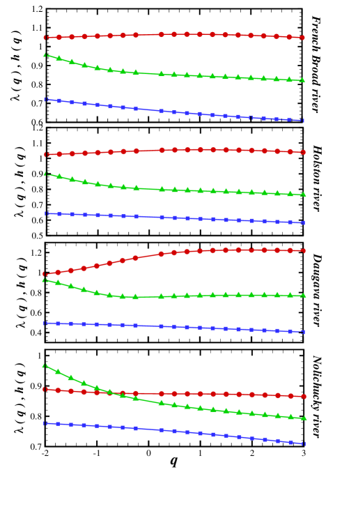
FIG. 12.: Generalized Hurst exponent, $h(q)$ computed by MF-DFA (filled circle and square symbols) and $\lambda(q)$ derived by equation (9) in MF-DXA method (filled triangle symbol). Filled circle and square correspond to sunspot numbers and mentioned runoff river fluctuations, respectively.

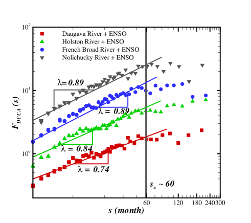
FIG. 13.: Fluctuation function versus scale in log-log plot computed by DCCA method for detrended river streamflows and El Niño index. To make more sense we shifted the vertical scale.

TABLE II.: Values of the scaling and cross-correlation exponents of detrended sunspot numbers and river flow fluctuations using the MF-DXA method for four rivers as well as scaling exponent given by the DFA method, $h(q)$, of each synchronized data set for $q=2$.

River	$h_{{\rm sunspot}}$	$h_{{\rm river}}$	$\lambda$	$\gamma_{\times}$
Nolichucky	$0.93\pm 0.01$	$0.70\pm 0.01$	$0.85\pm 0.01$	$0.30\pm 0.02$
French Broad	$1.11\pm 0.01$	$0.63\pm 0.01$	$0.84\pm 0.01$	$0.32\pm 0.02$
Holston	$1.05\pm 0.01$	$0.60\pm 0.01$	$0.78\pm 0.01$	$0.44\pm 0.02$
Daugava	$1.14\pm 0.01$	$0.61\pm 0.01$	$0.76\pm 0.01$	$0.48\pm 0.02$

To quantify the impact of El Niño (ENSO) phenomenon, we used the El Niño $3$ index reported in [82] since 1950. Applying SVD method, the sinusoidal trends have been diminished, thereafter, cleaned data sets used as inputs for DCCA algorithm. Figure (13) indicates the results computed by DCCA method for the detrended data sets. There is a crossover time scale in the fluctuation function as a function of scale for all underlying rives. The value of crossover equates to $s_{\times}\sim 60$ months which is so-called the period of El Niño phenomenon. The value of scaling exponents and cross-correlation exponents reported in Table III, confirm that on $s\leq 60$ months, there exists a cross-correlation between ENSO phenomenon and rivers. For time scale larger than $s>60$ months, this cross-correlation becomes ignorable [9, 10]. We also compare the impact of ENSO phenomenon and sun activity on the streamflow of rives. To this end, we should synchronize the El Niño, sunspot and river flow fluctuations. The value of scaling exponents and cross-correlation exponents for sunspot-river have also been reported in Table III. We find that the contribution of sun activity represented by sunspot is almost larger than ENSO phenomenon on the mentioned runoff rivers during mentioned period.

TABLE III.: Values of the scaling and cross-correlation exponents of synchronized El Niño 3 index and river flow fluctuations as well as for sunspot and river in the same period, using the DCCA method.

River	$\lambda_{\rm ENSO}$	$\gamma_{\times}^{\rm ENSO}$	$\lambda_{\rm sunspot}$	$\gamma_{\times}^{\rm sunspot}$
Nolichucky	$0.89\pm 0.03$	$0.22\pm 0.06$	$0.94\pm 0.01$	$0.12\pm 0.02$
French Broad	$0.89\pm 0.03$	$0.22\pm 0.06$	$0.98\pm 0.02$	$0.04\pm 0.02$
Holston	$0.85\pm 0.03$	$0.30\pm 0.06$	$0.90\pm 0.01$	$0.20\pm 0.02$
Daugava	$0.74\pm 0.03$	$0.52\pm 0.06$	$0.77\pm 0.01$	$0.46\pm 0.02$

IV Discussion and conclusion

There are many motivations such as complexity of fluctuations in our environments which lead to examine them using robust and novel methods from complex systems and statistical physics point of views. Knowledge of natural variabilities are necessary to manage the energy resources and prevent disasters from social and economical point of views. In this paper, we analyzed three important fluctuations in the nature, namely sun activity illustrated by sunspot numbers, El Niño phenomenon and streamflow of rivers. However, many climate indicators such as river flow fluctuations are affected by dominant seasonal trends, but recent researches have confirmed that, there are many variables causing the evolution of environmental conditions behave as a complex systems. Subsequently, applying the common methods in data analysis give incorrect or at least unreliable results. On the other hand to infer valuable results, the following necessary conditions should be satisfied:
i) The length of underlying time series should be large enough.
ii) The contribution of superimposed trends and noises on the recorded data must be small enough or at least distinguishable.
Unfortunately above necessary conditions cannot be met in some practical measurements. To solve these problems, we rely on the robust methods in data analysis to explore the mutual effect of sunspot and runoff water fluctuations. Based on the mentioned motivation, we apply the most recent method, Multifractal Detrended Cross-Correlation Analysis (MF-DXA), to examine the cross-correlation and fractal properties of sunspot numbers and river flow fluctuations for some most famous and available rivers.

Based on previous researches, as we expect, there are many sinusoidal trends embedded in the underlying signals. Unfortunately, these trends cannot be removed by common detrended procedures in DFA and DCCA analysis [47, 48]. These trends may cause some spurious crossovers in the fluctuations function versus time scale related to the competition between noise and trends. According to Figure (4), there are some crossovers in the fluctuation function of the sunspot numbers versus time scale,$s$. The first one corresponds to the annually period, the second is equal to the so-called solar activity, 11 years, while the last one may indicate the well-known Gleissberg period, but we must point out that this value with small uncertainty cannot be determined by this current data, because the size of data set is small. Here to eliminate those trends, we use the Singular Value Decomposition (SVD) method.

Results given by DFA method for original runoff rivers and sunspot numbers, demonstrated that all underlying runoff river behave as the anti-persistent long-range correlated series for time scale $s<12$ months at $1\sigma$ confidence interval (Figure (6)). On the other hand, the value of Hurst exponents for series without sinusoidal trends exhibit runoff rivers and sunspot numbers are long-range correlated process (see Table II).

MF-DXA analysis for non-detrended underlying data sets implied universal scaling exponent of fluctuation function for $q=2$ for all underlying rivers flow at intermediate time scales, $[12-24]\leq s\leq 130$ months, namely $\lambda=1.17\pm 0.04$ (see Figure (8)). This finding has recently been reported in Ref. [81] from power spectrum analysis. On the other hand there is a similar crossover in cross-correlation fluctuation functions at $s_{\times}\sim 130$ months which is known as cycle of solar activity, for all studied rivers versus sunspot [13].

Data without sinusoidal trends were used as the inputs for DCCA and its generalized MF-DXA methods. Due to the scaling behavior of fluctuations function (equation (9)) versus time scale, $s$, we concluded that there exists a significant cross-correlation between sun activity and water runoff river fluctuations. This cross-correlation confirms that the influence of other reasons on the river flow fluctuations such as human activity, drainage network morphology, land use patterns and topography may be ignored or at least cannot be distinguished form major effect which here is sun activity [81]. It must point out that, we know that the amount of radiation given off by the Sun (solar irradiance) is greatest when there are lots of sunspots. As discussed in detail in Ref. [9], the higher value of galactic cosmic ray, the higher the cloud cover which increases water resource of river, so we expect streamflow to be almost cross-correlated with solar activity. Other explanation are also investigated in [83, 84].

The cross-correlation exponent, $\gamma_{\times}$, of underlying data set in the presence of non-stationarities and trends have been determined by DCCA method. According to the relation between scaling exponent, $\lambda(q=2)$, and cross-correlation exponent, $\gamma_{\times}$, namely $\gamma_{\times}=2-2\lambda(q=2)$, one find that for long-range cross-correlated signals, the value of $\gamma_{\times}$ goes to small value demonstrating the cross-correlation function decreases more slowly and statistically two underlying data sets tend their present situation in their cross-correlation behavior. According to the values reported in Table II and Figures (10) and (11), there exists a long-range cross-correlation between rivers flow fluctuations used in this paper and sun activity indicated by sunspot numbers.

Weak $q$-dependency of the generalized Hurst, $h(q)$, and scaling, $\lambda(q)$, exponents, demonstrates that the original underlying series and also cross-correlation between sunspot numbers and each river behave as almost multifractal processes, demonstrating another universal characteristics. The value of $\lambda(q)$ for $q>0$ remains almost constant, this indicates that the rare events in the cross-correlation function behave in similar way. The similarity in behavior of fluctuation function, $F_{q}(s)$ in the MF-DXA method demonstrates the various type of fluctuations in different time scales have the same fractal features. Based on this result, this may be useful to extend the fractal properties of cross-correlation function derived by using short time scales to larger one without relying on the large time series. In addition, the rare events in streamflow and sunspot cross-correlation analysis, are not affected by local characteristics.

According to our results, the empirical relation between $\lambda(q=2)$ and Hurst exponent, $\lambda(q=2)\approx[h_{{\rm sun}}(q=2)+h_{{\rm river}}(q=2)]/2$, has also been confirmed.

Since the value of cross-correlation of Daugava river and sunspot numbers is less than other rivers, one can conclude that, beside the sun as a main resource of energy in the nature, the river’s geographical situation and the source of rainfall for that river may have reasonable impact on runoff water fluctuation. Recently, even an opposite behavior between solar activity and rainfall fluctuation in equatorial east Africa has been noticed in the recent report of the East Africa [85] explained in Ref. [9]. In addition, the value of $\lambda$ for French Broad and Nolichucky rivers are larger than two remained runoff rivers. Figure (9) also indicated, the power spectrum of French Broad and Nolichucky rivers behave in similar way around the well-known solar activity period. We also found a sharp crossover in the fluctuation functions derived by MF-DXA method for mentioned rivers in Figure (7). Since, the geographical positions of French Broad and Nolichucky rivers are close together, subsequently as expressed before, the impact of sun activity represented by sunspot, depends on the geographical properties of rivers.

One of the most important phenomenon which can affect the runoff rivers is El Niño (ENSO). To compare the contribution of ENSO phenomenon and sun activity, we used El Niño index $3$. The results derived by DCCA have been indicated in Figure (13) and also reported in Table III. There exists a crossover time scale in the log-log plot of fluctuation function versus scale. The value of this crossover time scale is $s_{\times}\sim 60$ months regarding to well-known ENSO period. ENSO phenomenon is cross-correlated by streamflow fluctuations for $s\leq 60$ months, while for larger than this period, one can ignore this cross-correlation behavior. By comparison, the effect of ENSO phenomenon and sun activity on the river flows, we found that the contribution of sunspot is almost larger than ENSO index since $1950$.

There are many methods to predict the sun activity [35, 36], so based on our current results which is demonstrated the cross-correlation between detrended sunspots and water runoff, one may use those results to predict river flow fluctuations.

Finally, one must point out that it should be interesting to extend the present analysis to a various set of runoff water fluctuations and other sun activity indicators such as solar irradiance, galactic cosmic rays flux and geomagnetic activity to find whether the values for the main parameters used in this analysis have a more universal validity of the solar influence on the streamflow fluctuations assigned as a climate variable in this paper.

Acknowledgements This research has been financially supported by Shahid Beheshti University research deputy affairs under grant No. 600/405.

REFERENCES

- [1] E. Koscielny-Bunde, A. Bunde, S. Havlin, H.E. Roman, Y. Goldreich, H.-J. Schellnhuber, Phys. Rev. Lett. 81, 729 (1998).
- [2] S.M. Barbosa, M.J. Fernandes and M.E. Silva, Physica A 371 (2006) 72573.
- [3] K. Fraedrich, U. Luksch, R. Blender, Phys. Rev. E 70 (2004) 037301.
- [4] W. B.White, J. Lean, D. R. Cayan, and M. D. Dettinger, J. Geophys. Res. 102, 3255 (1997).
- [5] W. B. White, Journal of Geophysical Research (Oceans) 111, 9020 (2006).
- [6] W. B.White and Z. Liu, Journal of Geophysical Research (Oceans) 113, 1002 (2008).
- [7] N. D. Marsh and H. Svensmark, Physical Review Letters 85, 5004 (2000).
- [8] B. Sun and R. S. Bradley, Journal of Geophysical Research (Atmospheres) 107, 4211 (2002).
- [9] P. J. D Mauas, E. Flamenco, A. P. Buccino, Phys.Rev.Lett. 101, 168501 (2008).
- [10] Pablo J.D. Mauas, Andrea P. Buccino and Eduardo Flamenco, Journal of Atomospheric and Solar-Terrestrial Physics, in press, arXiv:1003.0414.
- [11] V. Livina, Y. Ashkenazy, P. Braun, R. Monetti, A. Bunde and S. Havlin, Physical Review E, 67 (2003) 042101.
- [12] V. Livina et al., Physica A, 330 (2003) 283-290.
- [13] M. Sadegh Movahed and Evalds Hermanis, Physica A 387, 915 (2008).
- [14] Sergio Arianos and Anna Carbone, JSTAT, P03037 (2009).
- [15] Q. Zhang et al., Physics A, 388 (2009), 927-934.
- [16] R.U. Murdock, J.S. Gulliver, J. Water Res. Pl-Asce. 119 (1993) 473.
- [17] C.N. Kroll, R.M. Vogel, J. Hydrol. Eng. 7 (2003) 137.
- [18] H.E. Hurst, Transact. Am. Soc. Civil Eng. 116 770 (1951).
- [19] Y. Tessier, S. Lovejoy, P. Hubert, D. Schertzer, S. Pecknold, J. Geophys. Res. Atmos. 101 (1996) 26 427.
- [20] G. Pandey, S. Lovejoy, D. Schertzer, J. Hydrol. 208 (1998) 62.
- [21] J.D. Pelletier, D.L. Turcotte, J. Hydrol. 203 (1997) (14) 198.
- [22] E. Koscielny-Bunde, J.W. Kantelhardt, P. Braun, A. Bunde, S. Havlin, Proceedings of Conference Hydrofractals 2003, arXiv:physics/0305078.
- [23] J.W. Kantelhardt, D. Rybski, S.A. Zschiegner, P. Braun, E. Koscielny-Bunde, V. Livina, S. Havlin, A. Bunde, Physica A 330 (2003) doi:10.1016/j.physa.2003.08.019 [these proceedings].
- [24] Y. Ashkenazy et al., Phys. Rev. L., 86(9) (2001) 1900-1903.
- [25] Y. Ashkenazy et al., Physica A, 323 (2003) 19-41.
- [26] N. Loboda, Geophysical Research Abstracts, 8(2006) 00797.
- [27] A. Veronig, M. Messerotti and A. Hanslmeier, 2000 Astronomy and Astrophysics, 357, 337-350
- [28] V. I. Abramenko, 2005 Solar Physics, 228, 29-42
- [29] V. I. Zhukov, arXive:astro-ph/0304456.
- [30] M. Temmer, A. Veronig, 2002 J. Rybák and A. Hanslmeier, Proc. 10th. European Solar Physics Meeting
- [31] M. Temmer, A. Veronig and A. Hanslmeier, Astronomy and Astrophysics, 390, 707-715 (2002).
- [32] R. S. Bogart, 1982 Solar Physics, 76, 155
- [33] M. Temmer and et. al., Astronomy and Astrophysics, 392-2, 699-712 (2002).
- [34] M. Temmer, A. Veronig and A. Hanslmeier, 2003 Solar Physics, 512, 111-129
- [35] D.J.R. Nordemann, N.R. Rigozo, M.P. de Souza Echer, E. Echer, Computers & Geosciences 34 (2008) 1443 1453.
- [36] M. Li, K. Mehrotra, C. Mohan, S. Ranka, Intelligent Control Proceedings., 5th IEEE International Symposium on 5-7 Sept. Page(s):524 - 529 vol.1 (1990).
- [37] L. A. Balmaceda, S. K. Solanki and N. A. Krivova, JOURNAL OF GEOPHYSICAL RESEARCH, VOL. 114, A07104, 12 PP., 2009.
- [38] A. Tritschler, arXiv:0903.1300
- [39] F. Schmitt, D. La Valle, and D. Schertzer Phys. Rev. Lett. 68 (1992) 305308.
- [40] P. Burlando, e R. Rosso, J. Hydrol., vol. 187/1-2 (1996) 45-64.
- [41] P. Burlando, A. Montanari, e R. Rosso, (1996) Modelling hydrological data with and without long memory, Meccanica, 31, pp.87-101, Kluwer Ac. Publ., Dordrecht, The Netherlands.
- [42] Joanna D. Haigh, Climate and Weather of the Sun-Earth System(CAWSES): Selected Papers from the 2007 Kyoto Symposium, Edited by T. Tsuda, R. Fujii, K. Shibata, and M. A. Geller, pp. 231256.
- [43] B.B. Mandelbrot, J.R. Wallis, Water Resour. Res. 5 (1969) 321.
- [44] H.E. Hurst, R.P. Black and Y.M. Simaika, 1965 Long-term storage. An experimental study (Constable, London).
- [45] J. Feder, Fractals, Plenum Press, New York, 1988.
- [46] C. Matsoukas, S. Islam, I. Rodriguez-Iturbe, J. Geophys. Res. Atmos. 105 (2000) 29 165.
- [47] K. Hu, P. Ch. Ivanov, Z. Chen, P. Carpena and H. E. Stanley, Phys. Rev. E 64, 011114 (2001).
- [48] Zhi Chen, Plamen Ch. Ivanov, Kun Hu, H. Eugene Stanley, Phys. Rev. E 65, 041107 (2002).
- [49] B. Podobnik and H. Euge Stanley, Phys. Rev. Lett. 100, 084102 (2008).
- [50] Wei-Xing Zhou, Phys. Rev. E 77, 066211 (2008).
- [51] C. K. Peng, S. Havlin, H. E. Stanley and A. L. Goldberger, Chaos 5, 82 (1995).
- [52] J. W. kantelhardt, S. A. Zschiegner, E. Koscielny-Bunde, A. Bunde, S. Havlin and H. E. Stanley, Physica A 316, 87 (2002).
- [53] R. N. Mantegna and H. E. Stanley, “An Introduction to Econophysics” (Cambridge University Press, Cambridge, 2000).
- [54] Y. Liu, P. Gopikrishnan, P. Cizeau, M. Meyer, C. K. Peng and H. E. Stanley, Phys. Rev. E 60, 1390 (1999).
- [55] N. Vandewalle, M. Ausloos and P. Boveroux, Physica A 269, 170 (1999).
- [56] P. C. Ivanov, A. Yuen, B. Podobnik, Y. Lee, Phys. Rev. E 69, 056107 (2004).
- [57] M. Sadegh Movahed, G. R. Jafari, F. Ghasemi, S. Rahvar and M. Rahimi Tabar, J. Stat. Mech, P02003 (2006).
- [58] Jing Hu, Jianbo Gao and Xingsong Wang, J. Stat. Mech, P02066 (2009).
- [59] M. Sadegh Movahed, F. Ghasemi, S. Rahvar and M. Rahimi Tabar, arXiv:astro-ph/0602461
- [60] G. R. Jafari, P. Pedram, L. Hedayatifar, J. Stat. Mech, P04012 (2007)
- [61] Heather D. Jennings, Plamen Ch. Ivanov, Allande M. Martins, P. C. da Silva and G.M. Viswanathan, Physica A 336, 585 (2004).
- [62] S. Kimiagar, M. Sadegh Movahed, S. Khorram, S. Sobhanian and M. Reza Rahimi Tabar, J. Stat. Mech.(2009) P03020.
- [63] Jun et al. Phys. Rev. E 73, 066128 (2006).
- [64] C. V. Chianca, A. Ticona and T. J. P. Penna, Physica A 357, 447 (2005).
- [65] Radhakrishnan Nagarajan and Rajesh G. Kavasseri, Chaos, Solitons and Fractals 26, 777784 (2005).
- [66] Radhakrishnan Nagarajan and Rajesh G. Kavasseri, Physica A 354, 182198 (2005).
- [67] S. Shadkhoo and G.R. Jafari, Eur. Phys. J. B 72, 679-683 (2009).
- [68] A. Bunde, S. Havlin, J. W. Kantelhardt, T. Penzel, J. H. Peter and K. Voigt, Phys. Rev. Lett. 85, 3736 (2000).
- [69] Jr. R. Colistete , J.C. Fabris, S. V. B. Goncalves and P. E. de Souza , Int. J. Mod. Phys. D 13, 669 (2004)
- [70] Z. Wu et. al., PNAS, 104, 38, p. 14889-14894(2007)
- [71] J. W. Kantelhardt, E. Koscielny-Bunde, H. H. A. Rego, S. Havlin and A. Bunde, Physica A 295, 441 (2001).
- [72] G. Golub, C. van Loan, Matrix Computations, third ed., The Johns Hopkins University Press Ltd., London, 1996.
- [73] J. W. Cooley and J.W. Tukey , Mathematics of Computation, 19, 297 (1965).
- [74] R. Nagarajan and R. G. Kavasseri, Int. Journal of Bifurcations and Chaos, 15, no.2, (2005).
- [75] E. Koscielny-Bunde, H. E. Roman, A. Bunde, S. Havlin and H. J. Schellnhuber, Phil. Mag. B 77, 1331 (1998).
- [76] Pengjian Shang, Aijing Lin and Liang Liu, Physica A 388(2009) 720-726.
-
[77]
http://ftp.ngdc.noaa.gov/STP/SOLARDATA
/SUNSPOTNUMBERS - [78] http://sidc.oma.be
- [79] http://waterdata.usgs.gov
- [80] http://www.meteo.lv/public/26902.html
- [81] Zanchettin, D., A. Rubino, P. Traverso, and M. Tomasino, J. Geophys. Res., 113, D12102 (2008).
-
[82]
http://www.cpc.ncep.noaa.gov/data/indices
/sstoi.indices. - [83] Bhattacharyya, Subarna; Narasimha, Roddam, J. Geophys. Res., Vol. 112, No. D24, D24103 (2007).
- [84] Ruzmaikin, A., Feynman, J., Yung, Y.L., Journal of Geophysical Research (Atmospheres) 111 21114(2006).
- [85] D. Verschuren, K. R. Laird, and B. F. Cumming, Nature (London) 403, 410 (2000).