Estimating the selection efficiency

Abstract

The measurement of the efficiency of an event selection is always an important part of the analysis of experimental data. The statistical techniques which are needed to determine the efficiency and its uncertainty are reviewed. Frequentist and Bayesian approaches are illustrated, and the problem of choosing a meaningful prior is explicitly addressed. Several practical use cases are considered, from the problem of combining different samples to complex situations in which non-unit weights or non-independent selections have been used.

1 Introduction

There are several cases in high-energy physics (HEP) in which one has to measure a selection efficiency, for example when dealing with the trigger or offline event selection with the aim of measuring a cross section. The selection efficiency is the conditional probability that any single event passes the selection, given all other conditions (type and energy of the collisions, detector configuration, and possibly a preselection). A good estimator of the selection efficiency is the measured success frequency, that is the ratio between the number of surviving events and the size of the initial sample, which for larger and larger samples converges in probability to the selection efficiency (Bernoulli’s theorem). Different ways of summarizing the uncertainty on the true efficiency exist, as explained below, within the frameworks of the traditional (frequentist) and of the Bayesian approaches.

A short comparison between the two approaches is provided in [1, chapter 32] and a more complete comparison can be found in [2, appendix B]. The frequentist approach, often preferred in HEP data analysis, is fully reviewed by [3], including the open issues related to the possibility of choosing among different solutions for the same problem. Although in the Bayesian framework there is only one way of finding the solution, freedom remains in the choice of the prior, as it will be discussed below.

The most important difference among the two approaches is the kind of question they address. In the classical approach, the typical answer is in terms of the probability of obtaining some result, given the model. On the other hand, the Bayesian approach answers questions about the probability that some hypothesis is true, given the observed data. Hence, once the question is formulated in terms of either the probability of the data given the model or the probability of the hypothesis given the observation, one knows which approach is to be selected. In our case, the statistical inference deals with the unknown value of the parameter of interest, the selection efficiency. In the Bayesian approach, this is reduced to a problem of probability, because the framework provides the solution in terms of the probability distribution of the unknown parameter (interpreted as a description of the experimenter’s degree of belief on the possible values) given the observation. On the other hand, this probability distribution is not even defined in the frequentist approach, in which one considers instead (hypothetical) identical repetitions of the same experiment and looks at the fraction of times in which the result is expected to be compatible with the (unknown) true value.

In most practical problems, the experimenter needs either a single value (the best estimate of the efficiency), to be used in the computation of the cross section, or a “reasonable” interval which is supposed to contain the true (unknown) value with high probability, to be used when reporting the result. In the frequentist approach, such interval is reported in the form of a confidence interval associated to its coverage, for example a 68.3% or a 95% confidence interval. This is interpreted in terms of identical repetitions: a coverage of $q$ means that, in the limit of a very high number of replications, the fraction of intervals (constructed in the same way) which contain the true value is $q$. It is important to note that this does not mean — as it is sometimes implicitly assumed — that the true value has $q$ probability of being contained by the reported interval. In contrast, this is exactly the interpretation of a $q$-credible interval obtained in the Bayesian framework. When the sample size is very large, the Bayesian $q$-credible intervals will have also coverage of $q$, although the rapidity of this convergence is different for different choices of the prior.

Our model can be considered a (possibly infinite) sequence $r_{1},r_{2},\ldots\in\{0,1\}$ of Bernoulli’s random variables which either posses or not a given property. The selection process consists in discarding those “events” which do not have that property, and the selection efficiency corresponds to the long run relative frequency $k/n$ where $k=\sum_{i=1}^{n}r_{n}$ is the total number of surviving events out of the initial $n$ events. This is the result of the Bernoulli’s theorem, also known as the “weak law of large numbers”: the relative frequency will converge in probability to the true efficiency in the limit of an infinite number $n$ of measurements.

In the usual case in which the total number $n$ of initial events is fixed independently from $k$ (for example, when it depends on the accelerator or detector live time), the probability of selecting $k$ events, given the sample size $n$ and the selection efficiency $\varepsilon$, is given by the binomial distribution

$$P(k|\varepsilon,n)=\mathrm{Bi}(k|\varepsilon,n)\equiv\binom{n}{k}\varepsilon^{k}(1-\varepsilon)^{n-k}\;.$$ (1)

The likelihood function of the model $L(\varepsilon;n,k)$ is also given by (1), in which $\mathrm{Bi}(k|\varepsilon,n)$ is interpreted as a function of the unknown efficiency $\varepsilon$ with data fixed at the observed counts $k$ given $n$.

In the (less common) cases in which one continues performing the selection until $r\geq 1$ events are collected, the probability model is the negative binomial distribution:

$$P(n|\varepsilon,r)=\text{Nb}(n|\varepsilon,r)\equiv\binom{n-1}{r-1}\varepsilon^{r}(1-\varepsilon)^{n-r}$$ (2)

with $n=r,r+1,r+2,\ldots$

The frequentist approach is summarized is section 2 whereas the Bayesian approach is explained in section 3. Finally, several use cases are considered in detail in section 4.

2 The classical approach

Most often, we deal with the binomial model and are interested into the selection efficiency as a function of some measured quantity $x$, which can be a scalar (e.g. the missing transverse momentum in the event) or a multidimensional parameter (e.g. the magnitude of the transverse momentum and the two angles defining the direction of a reconstructed electron). In practice, we fill histograms of $x$ before and after the selection $S$ and compare the entries $k_{i}$ (surviving the selection $A$) and $n_{i}$ (initial counts) in each bin $i$. A bin-wise ratio of the histograms filled after and before the selection will result into the histogram of the success frequencies $f_{i}=k_{i}/n_{i}$, which, by virtue of Bernoulli’s theorem, can be taken as the estimates of the unknown efficiencies $\varepsilon_{i}$ (the histograms must be filled with unit weights for this to be true):

$$\varepsilon_{i}\equiv\int_{\text{bin $i$}}\varepsilon(x;A)\,\mathrm{d}x\;\approx\;f_{i}(A)\equiv\frac{k_{i}(A)}{n_{i}}$$

where we use the symbol $\approx$ to mean “is estimated by”. In the following, we will omit the bin index ($i$) and the selection ($A$) for simplicity.

The frequency $f$ is also the maximum likelihood estimator (MLE) for this problem, i.e. the value of $\varepsilon$ which maximizes the likelihood function (1). The MLE $f$ of $\varepsilon$ is an unbiased estimator with a number of attractive asymptotic properties [4, 5], which justify its widespread use:

• Consistency: the MLE converges in probability to the true value;

• Asymptotic normality: the distribution of the MLE tends to the Gaussian distribution centred on the true value for very large sample sizes $n$;

• Efficiency: the MLE achieves the Cramér-Rao lower bound (no asymptotically unbiased estimator has lower asymptotic mean squared error than the MLE).

For the MLE $\hat{}\varepsilon$ of a Bernoulli’s process, the Cramér-Rao lower bound is

$$V(\hat{}\varepsilon)=\frac{1}{I(\varepsilon)}=\frac{\varepsilon(1-\varepsilon)}{n}=\frac{V(k)}{n^{2}}=V(f)$$

where $I(\varepsilon)=\sum_{k}\mathrm{Bi}(k|\varepsilon,n)[\partial\log\mathrm{Bi}(k|\varepsilon,n)/\partial\varepsilon]^{2}=n[\varepsilon(1-\varepsilon)]^{-1}$ is the Fisher information, and the last expression follows from the property $V(ax)=a^{2}\,V(x)$, when $a$ is a known constant. By replacing $\varepsilon$ with the observed success frequency $f$ one obtains the widely (ab)used approximation

$$V(\hat{}\varepsilon)\approx f(1-f)/n=k(n-k)/n^{3}\;.$$ (3)

The asymptotic properties are approximately valid also for moderately large values of both $k$ and $n$, and this is the reason why the MLE $f$ and its approximate asymptotic uncertainty $\sigma_{f}=\sqrt{f(1-f)/n}$ are used so often. However, they do not hold any more for small $n$ and when $k=0$ or $n$ (even if $n$ is large!). For example, the asymptotic variance is zero when $k=n$ (which makes sense for $n\to\infty$ because it means that the true value is $\varepsilon=1$), but this is clearly a bad estimate of the uncertainty for any finite value of $n$: it would assign the same (zero) uncertainty to $k=n=1$ and $k=n=100$, even though one naively expects the latter result to be 10 times more precise than the former. Finally, the confidence intervals $[f-\sigma_{f},f+\sigma_{f}]$ have not always the correct coverage and, most important, may exceed the allowed boundaries of $\varepsilon\in[0,1]$.

To overcome these difficulties, several frequentist recipes have been proposed [6, 3], and the most common ones are available in ROOT [7] as different options of the class TEfficiency. Due to the discrete nature of the problem, obtaining the desired coverage for all possible values of $(n,\varepsilon)$ is impossible. The well known Clopper-Pearson confidence intervals never undercover hence they are to be preferred in conservative analyses, but are considered too wide by many experts, who proposed alternative recipes which provide the correct coverage on the average, allowing for some degree of under-coverage. Usually, such approximations (illustrated in details in [6, 3]) look quite similar in practical applications, and are often indistinguishable from the Bayesian reference credible intervals explained below.

In HEP, people usually prefer to be conservative: wider confidence intervals which are known to never undercover are preferred in most situations. However, while this can be critical in the Poisson case which is relevant for the search of new phenomena [8, 9], it may be argued that it is not as essential in the case of efficiency estimation. When some approximate coverage is an accetable solution, as it looks reasonable for the specific case of interest here, then the choice is amongst a rather wide spectrum of alternative approximations. As explained in details in ref. [3], if Clopper-Pearson $q$-confidence intervals (which never undercover) are considered unacceptably too wide and one is ready to accept methods leading to intervals which may undercover, one may choose the Agresti-Coull approximation, which seldom undercovers, or approaches which give the desired average coverage like the Wilson formula or the Bayesian posterior reference $q$-credible intervals discussed below. The last two recipes (Wilson and Bayesian intervals) give results which are numerically very similar: when they are considered acceptable approximations, our suggestion is to choose the Bayesian credible intervals because they can be interpreted intuitively in terms of the probability to contain the true unknown value.

3 The Bayesian approach

In the Bayesian approach, the full solution is represented by the posterior probability density $p(\varepsilon|k,n)$ of the parameter of interest $\varepsilon$ (the selection efficiency), interpreted as our degree of belief about the possible values which $\varepsilon$ can assume. The posterior density is obtained by means of the Bayes’ theorem:

$$p(\varepsilon|k,n)=N\,\mathrm{Bi}(k|\varepsilon,n)\,\pi(\varepsilon)$$ (4)

in which the likelihood function is the binomial distribution $\mathrm{Bi}(k|\varepsilon,n)$ from equation (1), viewed as a function of $\varepsilon$, and the normalization constant is

$$N=\frac{(n+1)\,B(k+1,n-k+1)\,B(a,b)}{B(a+k,b+n-k)}\;.$$ (5)

Foundations require that the prior density $\pi(\varepsilon)$ encodes all information available about $\varepsilon$ before performing the experiment. This kind of prior is often called “subjective” because it reflects the experimenter’s degree of belief about different values based on the information available before performing the experiment. Because such adjective is emotionally charged, here we prefer to call this kind of prior an “informative” prior instead, in contrast to the “least-informative” priors discussed below (which are elsewhere defined “objective”).

Because an informative prior is interpreted in terms of degree of belief, it must be a proper (i.e. integrable) prior. Whenever the experimenter does not feel very comfortable with a particular choice of prior, a sensitivity analysis has to be performed in which the solutions found by adopting different “reasonable” priors are compared. In addition, one has the option of comparing the solutions corresponding to informative and least-informative priors. In the large-sample limit, the final result will not depend significantly on the choice of the prior. Hence, comparing the results obtained with different priors is also a way of assessing to what degree this limit is approached.

If the prior is a function $\pi(\varepsilon)=\mathrm{Be}(\varepsilon|a,b)$ belonging to the Beta family (appendix A.2), which contains the conjugate priors for the binomial model, the posterior also belongs to the same family:

$$p(\varepsilon|k,n)=\mathrm{Bi}(k|\varepsilon,n)\,\mathrm{Be}(\varepsilon|a,b)=\mathrm{Be}(\varepsilon|k+a,n-k+b)$$ (6)

This simplifies the math considerably. Since (a) any regular function defined on $[0,1]$ can be obtained as a linear combination of Beta densities and (b) the linearity of the Bayes’ theorem assures that in this case the posterior will be a linear combination of the corresponding posterior Beta densities [2], from the mathematical point of view one can limit herself to the Beta priors, as it will be done in the following. This is of course by no means an excuse for not performing a sensitivity analysis: different priors can be treated either numerically or by expressing (or approximating) them as linear combinations of Beta densities.

3.1 Informative priors

As stated above, the prior should represent all information available before performing the experiment. A common case is when we only have limited prior information, for example some estimate of its expectation $E$ and variance $V$. In this case, we can define an approximate prior by finding the Beta density with the same mean and variance with the method of moments: the Beta parameters $a,b$ are found by solving the two equations

$$a = E\left[\frac{E(1-E)}{V}-1\right]$$ (7)

$$b = (1-E)\left[\frac{E(1-E)}{V}-1\right]$$ (8)

Subtleties arise when the term in square brackets becomes negative, i.e. when $E$ is very near to zero or one. In this case, one can use an approximate prior whose parameters $a,b$ can be found from the formulae for the mode and variance (appendix A.2). The resulting Beta density is either monotonically decreasing with a maximum at zero or monotonically increasing with a maximum at one. A unique Beta density is defined by $a,b$ found this way, hence one should also consider different choices of the prior (at least a least-informative prior) to check the sensitivity of the result.

Another example is when the prior knowledge is the result of a different experiment. In this case, the posterior density of the latter is used as the prior in equation (6) for the current experiment. Then Bayes’ theorem gives immediately the combined result of the two measurements.

A further example is the efficiency measurement performed with two runs carried on with the same accelerator and detector configurations. Let $N=n_{1}+n_{2}$ be the total number of events collected in the two runs and $K=k_{1}+k_{2}$ be the total number of surviving events, where the outcome of run $j$ can be summarized in the sufficient statistic $(n_{j},k_{j})$. With the prior $\mathrm{Be}(\varepsilon|a,b)$ used on the first run and the resulting posterior used as prior for the second run, one obtains:

$$\begin{split}p(\varepsilon|K,N)&=\mathrm{Bi}(k_{2}|\varepsilon,n_{2})\,\mathrm{Be}(\varepsilon|k_{1}+a,n_{1}-k_{1}+b)\\ &=\mathrm{Be}(\varepsilon|k_{2}+k_{1}+a,n_{2}-k_{2}+n_{1}-k_{1}+b)\\ &=\mathrm{Be}(\varepsilon|K+a,N-K+b)\end{split}$$

exactly the same result which corresponds to a single longer run defined as the union of both runs, as expected.

3.2 Objective Bayesian results

In HEP publications, it is often required to report results which only depend on the assumed model and on the observed data. In this case, the choice of a “least-informative” prior which aims at encoding the minimal amount of information about the parameter is recommended. The study of priors which guarantee “objective” results in the sense precised above is the subject of the Bayesian reference analysis [10]. Such priors are called reference priors and are formally defined such that they maximize the amount of missing prior information. The definition makes only use of the asymptotic properties of the probability model [11]. The resulting reference posteriors have the best coverage properties [12] in the sense that the posterior $q$-credible intervals obtained with any other prior achieve the coverage $q$ more slowly, for increasing sample sizes $n$. In other words, reference priors are the “probability matching” priors whose $q$-credible intervals achieve the coverage $q$ most quickly for increasing sample sizes.

For the binomial model, the reference prior coincides with the Jeffreys’ prior [13] and is $\pi(\varepsilon)=\text{Be}(\varepsilon|\frac{1}{2},\frac{1}{2})\propto\varepsilon^{-1/2}(1-\varepsilon)^{-1/2}$, which has two maxima at the extrema and a unique minimum at $\varepsilon=1/2$. This means that the reference posterior density for the unknown parameter is

$$p(\varepsilon|r,n)=\text{Be}(\varepsilon|r+\tfrac{1}{2},n-r+\tfrac{1}{2})\propto\varepsilon^{r-1/2}(1-\varepsilon)^{n-r-1/2}$$ (9)

which has mean $E(\varepsilon)=(r+\frac{1}{2})/(n+1)$, a biased estimator of the true efficiency, and variance $V(\varepsilon)=(r+\tfrac{1}{2})(n-r+\tfrac{1}{2})/[(n+1)^{2}(n+2)]$. The variance for $r=0$ or $r=n$ decreases as $n^{-2}$ for large sample sizes $n$, as one naively expects, hence does not pose the problems arising from the use of the asymptotic expression derived from the MLE variance, equation (3), although the two expressions converge for large sample sizes. Figure 1 shows the reference posterior densities for a small sample ($n=10$, left plot), which shows a clear asymmetry in most cases, and a moderately large sample ($n=100$, right plot), for which the (symmetric) asymptotic expression provides a good approximation whenever the observed frequency is not too near zero or one.

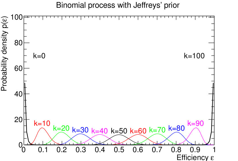
Figure 1: Reference posterior probability density function $\mathrm{Be}(\varepsilon;k+0.5,n-k+0.5)$ for $n=10$ (left) and $n=100$ (right).

Quite often, people have used the uniform prior $\mathrm{Be}(\varepsilon|1,1)$ in place of Jeffreys’ prior stating that the uniform prior is “non informative”. However this is not true in the binomial case, although one can find a 1:1 transformation $\psi=\psi(\varepsilon)$ such that the reference prior of the transformed variable $\psi$ is uniform (the reference parametrization) [10]: the transformation is $\psi(\varepsilon)=\frac{2}{\pi}\arcsin\sqrt{\varepsilon}$ whose inverse is $\varepsilon(\psi)=\sin^{2}(\psi\pi/2)$. In terms of the original parameter $\varepsilon$, the uniform prior is to be considered an informative prior. Incidentally, one can notice that the posterior mode is equal to the observed success frequency in this case, i.e. the posterior peak coincides with the MLE, because the whole posterior coincides with the likelihood function.

Our recommendation is to choose the reference prior when aiming at reporting results which only depend on the assumed model (the binomial process) and the observed data. However, the parameters of the posterior Beta density differ only by half unit when using the reference or the uniform prior. Hence in practice (unless the sample size is very small) there is not a big difference between the two posteriors. In particular, also the variance obtained with a uniform prior does not suffer from the problems of the asymptotic expression and gives similar results to the reference posterior variance already for $n=10$, as it appears from the comparison between figure 1, showing reference posteriors, and figure 2, showing the result obtained with a uniform prior for the same sample sizes.

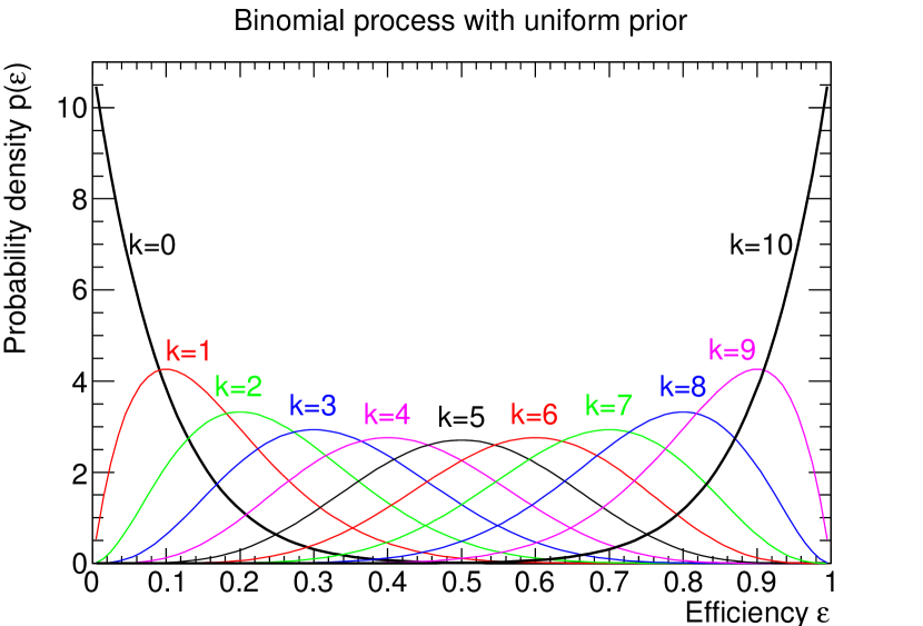
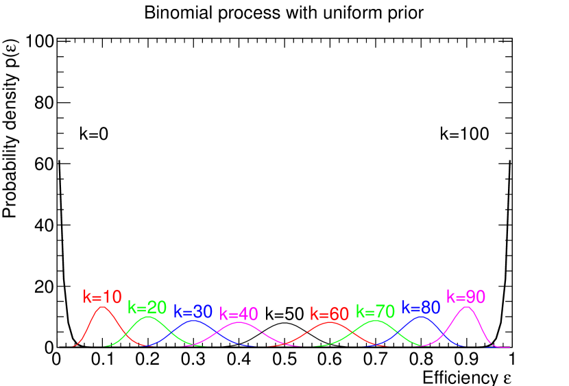
Figure 2: Posterior density $p(\varepsilon|k,n)=\mathrm{Be}(\varepsilon;k+1,n-k+1)$ obtained with the uniform prior, for $n=10$ (left) and $n=100$ (right).

The reference posterior mean and variance can be used in computations involving the efficiency, for example when estimating a cross section. The usual algebra of variances hold in this case, hence one can compute the best estimate of the cross section and its variance in the usual way. However, the posterior mean is not the only possibility for the “best” estimate. In addition, the posterior credible intervals are usually not symmetric about the mean. When these aspects are important, one should take into account what is treated in the following section.

3.3 Bayesian inference

In the Bayesian framework, the statistical inference is treated as a decision problem [14] in which one chooses the estimate which minimizes the posterior expected loss, for a suitably chosen loss function. Clearly, a very desirable property for an estimator $\varepsilon^{*}$ is the invariance under reparametrization, in the sense that the best estimator of a 1:1 function $\phi=\phi(\varepsilon)$ is $\phi^{*}=\phi(\varepsilon^{*})$. This is not achieved by the widespread quadratic loss, for which the best estimate is the posterior mean, because the quadratic loss is not invariant under reparametrization.

An example of invariant loss function is the $\mathcal{L}_{1}$ norm, that is the integral of the absolute value of the difference between two distributions, computed at the same point over the whole support. When applied to the reference posterior for the binomial case, the $\mathcal{L}_{1}$ norm gives the invariant expected loss

$$\ell_{1}\{\varepsilon_{0}|k,n\} = \int_{0}^{1}\ell_{1}(\varepsilon_{0},\varepsilon)\,\mathrm{Be}(\varepsilon|k+\tfrac{1}{2},n-k+\tfrac{1}{2})\,\mathrm{d}\varepsilon$$ (10)

$$\ell_{1}(\varepsilon_{0},\varepsilon) = \sum_{k=0}^{n}\left|\,\mathrm{Bi}(k|\varepsilon_{0},n)-\mathrm{Bi}(k|\varepsilon,n)\,\right|$$ (11)

independent from one-to-one transformations of $\varepsilon$. One can build a lowest posterior loss (LPL) $q$-credible region by finding the interval $[\varepsilon_{\text{low}},\varepsilon_{\text{up}}]\subset[0,1]$ which minimizes (10) under the constraint $\int_{\varepsilon_{\text{low}}}^{\varepsilon_{\text{up}}}\mathrm{Be}(\varepsilon|k+\tfrac{1}{2},n-k+\tfrac{1}{2})\,\mathrm{d}\varepsilon=q$.

The behaviour of many important limiting processes in probability theory and statistical inference is better described in terms of another measure of divergence, related to the information theory, the intrinsic discrepancy $\delta\{p_{1},p_{2}\}$, defined as the minimum among the two Kullback-Leibler directed divergences between two probability models $p_{1}$ and $p_{2}$ [14]:

$$\delta\{p_{1},p_{2}\} = \min\left\{\kappa\{p_{1},p_{2}\},\kappa\{p_{2},p_{1}\}\right\}$$ (12)

$$\kappa\{p_{i},p_{j}\} = \int_{\mathbb{X}}p_{i}(\vec{x})\log\frac{p_{i}(\vec{x})}{p_{j}(\vec{x})}\,\mathrm{d}\vec{x}$$ (13)

The intrinsic discrepancy is symmetric, non-negative, defined for strictly nested supports, invariant under one-to-one transformations, and additive for independent observations. It may be viewed as the minimum expected log-likelihood ratio in favour of the model which generates the data (the “true” model, which is assumed to be described either by $p_{1}$ or $p_{2}$) and can be used to defined the intrinsic discrepancy loss

$$\delta_{\vec{x}}\{\vec{\theta}_{0},\vec{\theta}\}=\delta\{p(\vec{x}|\vec{\theta}_{0}),p(\vec{x}|\vec{\theta})\}$$ (14)

where $\vec{\theta}$ is the parameter in which we are interested.

For the binomial model considered here $\vec{\theta}=\varepsilon$ and the intrinsic discrepancy loss is

$$\delta_{k}\{\varepsilon_{0},\varepsilon|n\} = n\,\delta\{\varepsilon_{0},\varepsilon\}$$ (15)

$$\delta\{\varepsilon_{0},\varepsilon\} = \min\left\{\kappa\{\varepsilon_{0}|\varepsilon\},\kappa\{\varepsilon|\varepsilon_{0}\}\right\}$$ (16)

$$\kappa\{\varepsilon_{i}|\varepsilon_{j}\} = \varepsilon_{j}\log\frac{\varepsilon_{j}}{\varepsilon_{i}}+(1-\varepsilon_{j})\log\frac{1-\varepsilon_{j}}{1-\varepsilon_{i}}$$ (17)

where $\delta\{\varepsilon_{0},\varepsilon\}$ is the intrinsic discrepancy between Bernoulli’s random variables with parameters $\varepsilon_{0}$ and $\varepsilon$.

The reference posterior expectation of the intrinsic discrepancy loss is the (reference posterior) intrinsic loss. The value $\vec{\theta}^{*}$ which minimizes the intrinsic loss is a Bayesian estimator which is called the intrinsic estimator of $\vec{\theta}$, and the reference posterior $q$-credible region which minimize the intrinsic loss is the intrinsic $q$-credible region of $\vec{\theta}$. Such credible regions are invariant under reparametrization and always contain $\vec{\theta}^{*}$, which is also invariant. In addition, the intrinsic $q$-credible regions are always approximate confidence regions with coverage $q$ and in some case they have the exact coverage, as it happens for location-scale models [12].

The intrinsic loss for the binomial model is

$$d(\varepsilon_{0}|k,n)=n\int_{0}^{1}\delta_{x}\{\varepsilon_{0},\varepsilon\}\,\mathrm{Be}(\varepsilon|k+\tfrac{1}{2},n-k+\tfrac{1}{2})\,\mathrm{d}\varepsilon$$ (18)

and the intrinsic estimator $\varepsilon^{*}$ is the value which minimizes equation (18). The intrinsic $q$-credible interval is the interval $[\varepsilon_{a}(k,n),\varepsilon_{b}(k,n)]\subset[0,1]$ which minimizes the loss (18) under the constraint $\int_{\varepsilon_{\text{low}}}^{\varepsilon_{\text{up}}}\mathrm{Be}(\varepsilon|k+\tfrac{1}{2},n-k+\tfrac{1}{2})\,\mathrm{d}\varepsilon=q$ (a simple numerical algorithm in suggested in appendix B). For the binomial model, because of its discrete nature, the exact coverage is not achieved for finite sample sizes, similarly to the confidence intervals obtained with the frequentist approach. One of the advantages of summarizing the result by providing $\varepsilon^{*}$ and the intrinsic interval $[\varepsilon_{a},\varepsilon_{b}]$ is that they are invariant under 1:1 reparametrization, in the sense that the intrinsic estimator of $\phi(\varepsilon)$ is $\phi(\varepsilon^{*})$ and its intrinsic $q$-credible interval is the $\phi$-image $\phi([\varepsilon_{a},\varepsilon_{b}])$ of $[\varepsilon_{a},\varepsilon_{b}]$. Hence, they are the recommended summaries of the full Bayesian solution (which is the reference posterior) when aiming at reporting an “objective” result.

A numerical treatment is needed to find the intrinsic estimator and the intrinsic credible intervals for the binomial model. However, one can obtain approximations good already with moderate sample sizes (say $n$ larger than few tens) by considering the approximate location parameter $\psi(\varepsilon)=\frac{2}{\pi}\arcsin\sqrt{\varepsilon}$ [10], such that the intrinsic estimator is

$$\varepsilon^{*}(k,n)\approx\sin^{2}\left(\frac{\pi}{2}E[\psi|k,n]\right)\approx\frac{k+\frac{1}{3}}{n+\frac{2}{3}}$$ (19)

(a very good approximation) and the reference posterior intrinsic loss is

$$d(\varepsilon_{0}|k,n)\approx\frac{1}{2}+2n\left[\arcsin\sqrt{\varepsilon_{0}}-\arcsin\sqrt{(k+\alpha_{n})/(n+2\alpha_{n})}\right]^{2}$$ (20)

where $\alpha_{n}=(n+4)/(4n+10)$ converges to $1/4$ for large $n$.

Simple (although less accurate) approximate expressions for the intrinsic credible intervals can be built upon the parametrization $\varepsilon(\phi)=\sin^{2}(\phi/2)$ [15]. Using a shorter notation for the reference posterior mean $\mu=E(\varepsilon)=(k+\tfrac{1}{2})/(n+1)$ and variance $\sigma^{2}=V(\varepsilon)=\mu(1-\mu)/(n+2)$ of the parameter of interest, the variance of the reference parametrization is

$$\sigma_{\phi}^{2}\approx\sigma^{2}[\phi^{\prime}(\mu)]^{2}=\frac{1}{n+2}$$ (21)

while its mean is

$$\begin{split}\mu_{\phi}&\approx\phi(\mu)+\frac{1}{2}\sigma^{2}\phi^{\prime\prime}(\mu)\\ &=2\arcsin\sqrt{\frac{k+\tfrac{1}{2}}{n+1}}+\frac{(2k-n)}{4(n+2)}\left[(k+\tfrac{1}{2})(n-k+\tfrac{1}{2})\right]^{-1/2}\end{split}$$ (22)

where $\phi^{\prime}$ and $\phi^{\prime\prime}$ denote the first and second derivative with respect to $\varepsilon$. Finally, the asymptotic intrinsic $q$-credible interval in the reference parametrization is $[\phi_{-},\phi_{+}]$ where

$$\phi_{\pm}\approx\mu_{\phi}\pm z_{q}\sigma_{\phi}=\mu_{\phi}\pm\frac{z_{q}}{\sqrt{n+2}}$$ (23)

where $z_{q}$ is the $(q+1)/2$ quantile of the normal distribution. The intrinsic $q$-credible interval for the efficiency is obtained by transforming back to $\varepsilon_{\pm}=\varepsilon(\phi_{\pm})=\sin^{2}(\phi_{\pm}/2)$.

Figure 3: Reference posterior intrinsic loss from the reference posterior expected loss (black dashed line) and its approximation (continuous red line) for a small sample size $n=10$. The triangles show the position of the minima of such functions and the vertical lines represent the limits of the 68.3% intrinsic credible interval (which becomes automatically one-sided in the case $k=0$).

	Exact			Approx 1		Approx 2
$k/n$	$d_{\text{min}}$	$\varepsilon^{*}$	68,3% interv.	$\varepsilon(\mu_{\phi})$	68,3% interv.	$\varepsilon^{*}_{\text{app}}$	68,3% interv.
0/10	0.24	0.033	[0.000, 0.060]	0.028	[0.002, 0.082]	0.031	[0.000, 0.060]
1/10	0.36	0.124	[0.024, 0.193]	0.122	[0.054, 0.211]	0.125	[0.024, 0.193]
2/10	0.40	0.218	[0.090, 0.326]	0.216	[0.125, 0.323]	0.219	[0.090, 0.326]
3/10	0.42	0.314	[0.171, 0.446]	0.311	[0.205, 0.427]	0.313	[0.169, 0.443]
4/10	0.43	0.408	[0.257, 0.552]	0.405	[0.290, 0.526]	0.406	[0.257, 0.552]
5/10	0.43	0.500	[0.350, 0.651]	0.500	[0.380, 0.620]	0.500	[0.350, 0.651]

Table 1: For a small sample size $n=10$, the minimum value of the reference posterior intrinsic loss, the intrinsic estimator and the intrinsic 68.3% credible interval from the exact definition eq. (3.13) are reported. Next, the approximated quantities derived from the reference parametrization $\varepsilon(\mu_{\phi})$ from eq. (3.17) and $\varepsilon(\phi_{\pm})$ from eq. (3.18) are shown. Finally, the approximate intrinsic estimator $\varepsilon^{*}_{\text{app}}=(k+1/3)/(n+2/3)$ from eq. (3.14) and the 68.3% credible interval from the approximate intrinsic loss defined by eq. (3.15) are reported, both representing a very good approximation.

Figure 3 shows the comparison between the correct [eq. (18)] and approximate [eq. (20)] intrinsic loss functions and table 1 reports the results obtained with them and with the reference parametrization. A small sample size $n=10$ is chosen such that these approximations give different results when reporting three decimal places and the values corresponding to $k=6,\ldots,10$ are omitted because they are symmetrical with respect to those obtained for $k=0,\ldots,5$. The overall agreement is fairly good even with such small sample.

The value $\varepsilon^{*}_{\text{app}}=(k+1/3)/(n+2/3)$ which minimizes the approximate intrinsic loss defined by eq. (20) provides a very good approximation to the exact intrinsic estimator $\varepsilon^{*}$ and the intervals (numerically) computed from the approximate intrinsic loss are practically the same as the exact intrinsic intervals, despite from the very small sample size $n=10$. The approximate quantities computed from the mean $\mu_{\phi}$ of the reference parametrization [eq. (22] and from its approximate credible intervals from eq. (23) are less good for such a small sample size, but become better with larger $n$. If their accuracy is considered acceptable, the approximate credible intervals from eq. (23) may be used together with $\varepsilon^{*}_{\text{app}}$ to provide a summary of the posterior which does not require a numerical algorithm to be developed to minimize the loss.

As mentioned above, the binomial model is discrete, hence the coverage is never exact. The intrinsic $q$-credible intervals are also approximate confidence intervals with coverage $q$, which may undercover or overcover depending on the actual values of $(n,\varepsilon)$, similarly to the approximate frequentist confidence intervals reviewed in [3]. This justifies the use of the approximate intrinsic intervals already for moderate sample sizes in all the cases in which an approximate coverage is accepted (that is when the Bayesian approach is chosen or when the frequentist approximate confidence intervals are considered acceptable approximations).

4 Non trivial use cases

So far, we assumed that all entries of the initial histogram had unit weight and that the events had been selected by an independent process, whose efficiency is completely uncorrelated with respect to the efficiency of the process under study (which means that it is expected to reduce the total number of events and the number of selected events in such a way that the long run success frequency remains unchanged). This is required to obtain a binomial process, but may not be true in all cases, as it happens sometimes in HEP problems.

For example, if the initial sample was obtained by scaling the simulated data sample to normalize it to some different value of the cross section, it should not be used to make efficiency studies! Rather, the efficiency should be estimated by using the original sample (with unit weights), in order to have a binomial process. Once the efficiency is known, it may be applied to the scaled distribution to estimate the total number of surviving events.

The following common examples are addressed in detail below.

1. Sometimes one is interested into the overall selection efficiency for a weighted mixture of different samples. This is a common use case in HEP, because Monte Carlo (MC) generators are often used to produce independent samples for different processes which greatly differ in their cross section, and is addressed below in section 4.1. Another common example in HEP is the output of MC@NLO [16], a mixture of events with weights $\pm 1$ (section 4.2).

2. When measuring the trigger efficiency, the initial sample might be selected by a non independent process. This happens for example when a random trigger provides not enough events to allow for studying the efficiency of the trigger of interest, and is addressed in section 4.3.

The most important assumption in the efficiency estimation methods considered here is that each individual event can be considered as a Bernoulli trial which contributes with either zero or one success to the count of surviving events. This gives the binomial likelihood, which is the starting point for both fequentist and Bayesian methods. The only case in which weighted events can be reconduced to the binomial scheme is when only integer weights are allowed, with the interpretation that an event with weight $m$ is just a short-hand notation for a set of $m$ Bernoulli’s trials all either passing or failing the selection. In this case, the likelihood for such events is just the product of $m$ identical likelihoods, that is the $m$-th power of the Bernoulli’s model. Moving from integer to real weights by assuming that the form of the likelihood is unchanged requires a mathematical proof which is unknown to the author.

In section 8.5 of James’ book [5] an approximate likelihood is described which uses real weights but requires quite some care because of its “paradoxical results”. One delicate point of his approach is that the variance of the estimator may be reduced by dropping events (in particular, those with large weights). The TEfficiency class offered by the ROOT framework implements it, allowing for arbitrary event weights, possibly dependent on some event property or observable quantity. However, this is not considered further in this article, in which we restrict the problem to a smaller set of use cases (in which the solutions proposed below are practically equivalent to the result obtained with TEfficiency).

Here we only consider situations in which we have a finite number $s$ of possible event sets (or classifications), and the event weights only depend on $s$, which implies that they can only assume $s$ possible values $w_{1},\ldots,w_{s}$ with probabilities $p_{i}$ satisfying $\sum_{i=1}^{s}p_{i}=1$. More explicitly, we do not consider weights which depend on some continuous observable quantity, nor the case of infinite countable weights.

The general case of unknown classification (which holds for the experimental data) cannot be fully solved, even when the probabilities $p_{i}$ (associated to all possible $s$ channels) are all known. In this case the sample consists of $N$ events and one has a multinomial distribution which relates the sizes $n_{1}+\ldots+n_{s}=N$ of the $s$ categories to the corresponding probabilities $p_{1},\ldots,p_{s}$, and a binomial term for each category which relates the number $k_{i}$ of events surviving the selection out of the initial $n_{i}$ events to the subsample efficiency $\varepsilon_{i}$. In other words, the likelihood is proportional to the product

$$P(k_{1},\ldots,k_{s};n_{1},\ldots,n_{s};\varepsilon_{1},\ldots,\varepsilon_{s})\propto\frac{N!\,p_{1}^{n_{1}}\cdots p_{s}^{n_{s}}}{n_{1}!\dots n_{s}!}\,\prod_{i=1}^{s}\binom{n_{i}}{k_{i}}\varepsilon^{k_{i}}(1-\varepsilon)^{n_{i}-k_{i}}$$ (24)

of a multinomial distribution which gives the probability of each partition $n_{1}+\ldots+n_{s}=N$ and $s$ binomial terms which express the probability of selecting all possible $s$-tuples $(0\leq k_{1}\leq n_{1}$, $\ldots$, $0\leq k_{s}\leq n_{s})$ such that $\sum_{i=1}^{s}k_{i}=K$. Because the only observable numbers are the initial sample size $N$ and the number $K$ of events passing the selection, even after the sum over all possible $s$-tuples $(n_{1},\ldots,n_{s})$ and $(k_{1},\ldots,k_{s})$, we are left with a $s$-dimensional problem in which the efficiencies $\varepsilon_{1},\ldots,\varepsilon_{s}$ cannot be determined, unless they satisfy some relation known a priori which allows to remove (or integrate over) $s-1$ degrees of freedom.

A common practical problem is the combination of several MC samples which correspond to independent physical processes, with known cross-sections. In this situation, the classification of each event and the probabilities $p_{i}$ are known: the file name provides the classification and both the weight $w_{i}$ and the probability $p_{i}=w_{i}/\sum_{i=1}^{s}w_{i}$ are proportional to the cross-section. Hence the general likelihood (24) is reduced to the product of independent binomial factors with known initial ($n_{i}$) and final ($k_{i}$) numbers of events and unknown efficiencies. This splits into a collection of individual problems: we can estimate the selection efficiency for each possible class as explained above, and compute the overall efficiency for the weighted mixture as illustrated in section 4.1 below.

In the particular case of MC@NLO we have $s=2$ categories to which any event can be associated thanks to the weights $w_{1}\equiv w_{+}=+1$ and $w_{2}\equiv w_{-}=-1$ assigned by the generator. From the user perspective the corresponding probabilities $p_{\pm}$ are unknown, although they can be estimated by looking at the ratio between the number $n_{\pm}$ of events in each category and the total number $n_{+}+n_{-}$ of generated events. Anyway, we are not interested into the values of $p_{\pm}$ themselves hence we can integrate (24) over them. This way, the marginal model has a likelihood function which only depends on the single-sample efficiencies $\varepsilon_{\pm}$ and this becomes a particular case of the problem mentioned above (more details on section 4.2 below).

4.1 Overall efficiency for mixed samples

A frequently encountered problem in HEP occurs when simulating concurrent processes with different cross sections. Interesting observables like the transverse momentum of electrons or jets may have distributions which decrease so rapidly that producing fully simulated samples with enough events in the whole interesting range (especially in the tail) is impractical, unless one splits the generator-level input into different samples with roughly the same size but different ranges (for example starting from a $\boldsymbol{p}_{\text{T}}$ value which doubles in each sample). In order to obtain a smooth distribution, such samples need to be mixed with weights which are proportional to their relative cross-sections.

Let us consider a finite number $s$ of independently generated samples with sizes $N_{i}$, $i=1,\ldots,s$ whose weights $w_{i}>0$ are perfectly known. Before the selection, the effective sample size is

$$N=\sum_{i}w_{i}N_{i}$$

where $N_{i}$ is the (known) initial size of the $i$-th sample.

Let $K_{i}$ be the known sample size after the selection and $\varepsilon_{i}$ be the unknown selection efficiency for the $i$-th sample. Then, the effective sample size after the selection is

$$K=\sum_{i}w_{i}K_{i}=\sum_{i}w_{i}N_{i}\varepsilon_{i}$$

and we are interested into the overall selection efficiency for the mixed sample.

Because all samples are independent, one can estimate the efficiency $\varepsilon_{i}$ and its variance $v_{i}$ for each sample separately, as explained in the previous sections. Next, the variance of $K$ can be computed with the usual algebra of variances:

$$V(K)=\sum_{i}w_{i}^{2}\,V(K_{i})=\sum_{i}(w_{i}N_{i})^{2}v_{i}\;.$$ (25)

When considering the mixed sample, one can estimate the unknown true efficiency by taking the ratio $E$ between $K$ and $N$:

$$E=\frac{K}{N}=\frac{\sum_{i}W_{i}\varepsilon_{i}}{\sum_{i}W_{i}}$$ (26)

which is a linear combination of the single-sample efficiencies $\varepsilon_{i}$ with weights $W_{i}=w_{i}N_{i}$. Its variance is

$$V=\left(\sum_{i}W_{i}^{2}v_{i}\right)/\left(\sum_{i}W_{i}\right)^{2}\;.$$ (27)

Instead of reporting $E\pm\sqrt{V}$, which would cause troubles if $E$ is too near zero or one, we may find the approximate asymmetric uncertainty band around the estimate $E$ by reporting the boundaries of a 68.3% credible region computed with the approximate Beta posterior for $E$ given by the method of moments, with inputs $E$ and $V$. Figure 4 shows that finding the approximate Beta posterior with the method of moments gives very good results even when the input single-sample efficiencies are significantly different. The overall efficiency has been estimated by performing 10000 repeated pseudo-experiments, and its distribution appears to be practically identical to the Beta density found with the method of moments. In this example, two small ($N_{1}=26$ and $N_{2}=10$ events) samples from populations with known weights ($w_{1}=0.7$ and $w_{2}=0.3$) and efficiencies ($\varepsilon_{1}=0.3$ and $\varepsilon_{2}=0.7$) have been mixed. The events passing the selection ($K_{1}=18$ and $K_{2}=3$) have been used to estimate the single-sample efficiencies, whose reference posterior densities are shown in the plot with a dashed red line and continuous blue line, respectively. The distribution obtained with the pseudo-experiments is best fitted by a Beta density with parameters $(25.64,18.97)$ and the approximate method gives a Beta posterior with parameters $(25.44,18.80)$, which is a very good approximation (the two curves overlap within their line width).

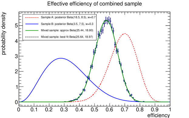
Figure 4: The overall efficiency for a selection carried on with a mixture of two samples with weights 70% and 30% and single-sample (true) efficiencies of 70% (18 selected out of 26 events) and 30% (3 selected out of 10 events) is estimated by performing 10000 repeated pseudo-experiments. The differences between the best fit and the approximate Beta density is not noticeable from the plot.

4.2 Events with positive or negative unit weights

In high-energy physics simulations, it might happen to work with simulated samples generated by MC@NLO [16], which assigns positive and negative (unit) events weights. Each individual event is independently simulated, and knows nothing about its weight. Hence we have two categories ($s=2$) with weights $w_{1}=+1$ and $w_{2}=-1$, initial sample sizes $N_{1}=n_{+},N_{2}=n_{-}$, and $K_{1}=k_{+},K_{2}=k_{-}$ entries after the selection.

For each sample, the efficiencies $\varepsilon_{+}$ and $\varepsilon_{-}$ can be computed individually and inserted into equations (26) and (27) above to obtain the overall efficiency estimate

$$E=\frac{\varepsilon_{+}n_{+}-\varepsilon_{-}n_{-}}{n_{+}-n_{-}}$$ (28)

with variance

$$V=\frac{n_{+}^{2}V(\varepsilon_{+})+n_{-}^{2}V(\varepsilon_{-})}{(n_{+}-n_{-})^{2}}$$ (29)

where $V(\varepsilon_{+})$ and $V(\varepsilon_{-})$ are the single-sample variances.

We note that equation (28) coincides with the recommendation by the MC@NLO authors when estimating the single-sample efficiency with the success frequency $f_{\pm}=k_{\pm}/n_{\pm}$. In Ref. [16] they say that the efficiency should be estimated as $f=(k_{+}-k_{-})/(n_{+}-n_{-})$ when $k_{+}\geq k_{-}$ or zero otherwise. This ration can be rewritten in a form $(f_{+}n_{+}-f_{-}n_{-})/(n_{+}-n_{-})$ which gives equation (28) with the replacement $f\to\varepsilon$. They also suggest to use the usual “propagation of errors” to estimate its variance whenever the numbers are high enough that the Gaussian approximation holds, or to run many MC samples through the cuts and look at the dispersion in the result if the data sample is too small. We have obtained equation (29) with the usual algebra of variances, and in the previous section we have seen that it can be used with the method of moments to find an approximate uncertainty band which is very close to the result obtained with pseudoesperiments (and does not require the Gaussian approximation to hold). It is sufficient to use equations (7) and (8) to find the approximated posterior Beta density, which can be used to plot the 68.3% intervals.

A fully Bayesian treatment of the difference between two independent random variables, each one following a Beta distribution, was performed by Pham-Gia, Turkkan & Eng [17], who found an analytical solution. There are few subtleties about their “beta-difference” distribution , which make it quite complicate to be used in the problem considered here:

• here we have a weighted difference $e_{+}-e_{-}$ where $e_{\pm}=n_{\pm}\varepsilon_{\pm}/(n_{+}-n_{-})$ can be considered “scaled” efficiencies;

• the general difference between two Beta-distributed variables has domain in $[-1,+1]$ whereas here we require it to be restricted to $[0,1]$ to have a physically meaningful quantity. This means that the beta-difference distribution has to be truncated at zero and renormalized, which requires a numerical treatment;

• a uniform prior is used (wrongly proposed as non-informative) to compute the beta-difference distribution, rather than a reference prior. This is not going to make a dramatic change, as shown in section 3.2 above, unless the sample size is very small.

Given the complexity of their formula and the necessity of accounting for the these complications, its seems much easier to proceed in the approximate method explained above, which is good (or at least acceptable) in most (practically all) common problems.

4.3 What to do if the samples are not independent?

The case in which the initial dataset does not represent a statistically independent sample is expecially important in trigger efficiency measurements, when there is no other trigger selection which is statistically uncorrelated with respect to the signature $A$ under study. Ideally, one would like to select the initial sample with a random trigger and then count how many events also survive the trigger $A$. However, for most interesting triggers a randomly collected sample contains practically no event which may satisfy them, making such random sampling useless. For this reason, some other trigger $B$ is used to select the initial sample, which is somewhat correlated with $A$ (for example, $B$ could be a trigger of the same type but looser than $A$). This correlation, which is necessary to select the initial sample such that there is some fraction of events passing $A$, must be accounted for explicitly when computing the efficiency of $A$.

The trigger efficiency $\varepsilon_{A}$ is the conditional probability that a single event, given all other conditions (collider settings, detector status and defects, calibration parameters, offline event selection, observables $\vec{x}$), is not rejected by $A$. In particular, it is fundamental to notice that different studies perform different offline event selections, such that the same trigger may have different efficiencies for each of them. Here we assume that the offline event selection is fixed, and we are interested into estimating the trigger efficiency $\varepsilon_{A}=P(A|\vec{x},\text{off.~{}sel.},\ldots)\equiv P(A)$ omitting all fixed conditions for brevity. The starting point is the sample of events which have been preselected by trigger $B$ and the same offline selection (with all other conditions fixed).

In order to find the desired efficiency $P(A)$, we make use of the relation defining the conditional probability, $P(A\cdot B)=P(A|B)\,P(B)=P(B|A)\,P(A)$, obtaining

$$P(A)=P(A|B)\,[P(B)/P(B|A)]\;,$$ (30)

where $P(A|B)$, the conditional trigger efficiency of $A$ for events which already passed $B$, can be estimated by taking the ratio between the final and initial (i.e. after $B$) sample sizes, as explained in the previous sections.

The fraction in square brackets cannot be determined with real data alone. Even when the trigger efficiency $P(B)$ is measured from real data, the conditional probability that the events pass $B$ given that $A$ is satisfied cannot clearly be estimated from real data. Simulated events are necessary to estimate $P(B|A)$ or the whole ratio $P(B)/P(B|A)$, in order to obtain an estimate of the desired trigger efficiency $P(A)$.

Usually, the auxiliary trigger $B$ is chosen in such a way that one can safely assume $P(B|A)=1$ with negligible uncertainty, by virtue of what is found with simulated samples. If this is the case, then the impact of the MC events is minimal: one additional measurement (performed with an independent sample) is required to find the trigger efficiency $P(B)$ of $B$ alone, together with the estimation of $P(A|B)$ with the sample preselected by $B$, in order to find $\varepsilon_{A}$ from equation (30). It is recommended to always check that the uncertainty on $P(B|A)=1$ is negligible with respect to the uncertainty associated to $P(A|B)$. If this is not the case, one can create an approximate model $P(B|A)$ with a monotonically increasing Beta density which peaks at one, and use the Bayes’ theorem to find the overall probability distribution for the parameter $\varepsilon_{A}$ of interest. Finding an approximate Beta density also works when $P(B|A)$ is not 100%, when the impact of the prior information coming from simulated samples is larger.

5 Summary

Estimating the selection efficiency is a fundamental task in most data analyses, based on simulated and/or real data. The measured success frequency provides the best estimate of the true efficiency in the frequentist approach (being the MLE) and coincides with the posterior mode obtained in the Bayesian treatment with the widely used uniform prior. However, such prior cannot be considered non-informative. Instead, if we are completely uncertain about the efficiency before making the experiment, or we aim at reporting “objective” Bayesian results, the use of the reference prior (which is the same as the Jeffreys’ prior in the binomial model) is recommended, together with the intrinsic estimators which have been reviewed in section 3.3.

Within the Bayesian approach, if some prior knowledge is available, for mathematical simplicity it is recommended to encode it into a function belonging to the family of Beta distributions, whose parameters can be determined with the method of moments if the exact function is not known. This ensures that the posterior also belongs to the same family, so that the math is simplified because all properties summarized in appendix A.2 are immediately available. An important example of the use of informative priors is the combination of independent samples, which is also used for including prior knowledge coming from simulations to model systematic effects.

The knowledge of the uncertainty about the efficiency is needed when scaling observed quantities to estimate their original values (e.g. the true rate). In this case, the easiest approach is to use the mean and variance of the posterior density in the computation, whenever the use of the full posterior is not practical. The usual variance algebra holds, with the caveat that the square root of the final variance might not be good to define a symmetric credible interval, because of the inherent asymmetry of the posterior in the general case. Though in many applications the posterior will be significantly peaked around the true value, so that the binomial (symmetric) approximation holds, care needs to be taken when handling very low or very high efficiencies, and when the number of events is relatively small, because such approximation behaves very poorly in such cases.

Several options for the confidence intervals are reviewed in [3], where it is emphasized that only the Clopper-Pearson $q$-confidence intervals never undercover. At the same time, they are considered too wide by many professional statisticians, who have proposed a number of recipes for defining confidence intervals with the desired average coverage but may undercover sometimes. Among the approximated confidence intervals, one may also select the Bayesian posterior $q$-credible intervals, which are numerically very similar to widely used frequentist approximations but have the advantage of a clear and unanbiguous interpretation in terms of the probability that the true unknown value is actually contained by them (which is not true for confidence intervals).

When plotting the result of an efficiency measurement, the observed frequency should be accompanied by asymmetric error bars. The TEfficiency class of the ROOT framework allows the user to choose among a number of options, including Clopper&Pearson confidence intervals, few frequentist approximated confidence intervals, and Bayesian credible intervals with different priors. If the coverage is considered an important aspect, then one should choose the Clopper&Pearson intervals. Otherwise, one may plot the Bayesian credible intervals obtained with the reference prior, which are also classical confidence intervals very similar to the Wilson approximation, achieving the desired coverage on the average (but not always). When the full probability model is not known and only mean and variance are available, acceptable intervals may be obtained (using TEfficiency) from the approximate Beta density with the same mean and variance, for illustration purposes.

Finally, special care must be used when handling samples that do not have unit weights or are not independent. Few recipes to deal with the most common use cases in particle physics have been sketched in section 4, including the case of weighted mixtures of MC samples with different cross sections. Approximate asymmetric uncertainty bands can be obtained in a simple way by finding the approximate Beta posterior with the method of moments. Finally, the measurement of the trigger efficiency starting from a sample which has been preselected by requiring another trigger which is not statistically independent is addressed, emphasizing the importance of a correct modeling of the relation between the two selections.

Appendix A Useful relations

This appendix summarizes mathematical definitions and properties that are useful when dealing with binomial processes. They can be found in standard books like [18, 2].

A.1 Gamma function

The Gamma function is defined on the complex plane ($z\in\mathbb{C}$):

$$\Gamma(z)=\int_{0}^{\infty}t^{z-1}e^{-t}\,\mathrm{d}t$$ (31)

with $\Gamma(z+1)=z\,\Gamma(z)$. For integer values, $\Gamma(n)=(n-1)!$.

A.2 Beta distribution

The Euler Beta function is a symmetric function of $a,b\in\mathbb{R}$:

$$B(a,b)\equiv\int_{0}^{1}t^{a-1}(1-t)^{b-1}\,\mathrm{d}t=\frac{\Gamma(a)\,\Gamma(b)}{\Gamma(a+b)}=B(b,a)$$ (32)

and the incomplete Beta function is

$$B_{x}(a,b)=\int_{0}^{x}t^{a-1}(1-t)^{b-1}\,\mathrm{d}t\;.$$ (33)

with $x\in[0,1]$.

For $x\in[0,1]$, the Beta distribution has probability density function

$$f(x;a,b)=\frac{1}{B(a,b)}x^{a-1}(1-x)^{b-1}\equiv\mathrm{Be}(x;a,b)$$ (34)

and cumulative distribution function

$$F(x;a,b)=\int_{0}^{x}f(t;a,b)\,\mathrm{d}t=\frac{B_{x}(a,b)}{B(a,b)}\equiv I_{x}(a,b)$$ (35)

where $I_{x}(a,b)=1-I_{1-x}(a,b)$ is the regularized incomplete Beta function. The mean $E$, mode $m$ (defined only for $a>1,b>1$), variance $V$ and skewness $\gamma_{1}$ of the Beta density (34) are

$$E(x;a,b) = \frac{a}{a+b}$$ (36)

$$m(x;a,b) = \frac{a-1}{a+b-2}$$ (37)

$$V(x;a,b) = \frac{ab}{(a+b)^{2}\,(a+b+1)}$$ (38)

$$\gamma_{1}(x;a,b) = \frac{2(b-a)\sqrt{a+b+1}}{(a+b+2)\sqrt{ab}}$$ (39)

When a single parameter is equal to one the density is monotonically decreasing or increasing with a unique maximum at $x=0$ or $x=1$; when $a=b=1$ one has the uniform distribution.

Finally, the characteristic function is

$$\phi(t)=\int_{0}^{1}\mathrm{Be}(x;a,b)\exp(-2\pi ixt)\,\mathrm{d}x={}_{1}F_{1}(a;a+b;it)$$ (40)

where ${}_{1}F_{1}(a;b;c)$ is the confluent hypergeometric function of the first kind.

Appendix B Computing intrinsic credible intervals

Although it is quite easy to find numerical libraries which minimize a function, finding posterior $q$-credible intervals which achieve the minimal expected posterior loss is not as simple. The intervals shown in this paper have been computed with a simple numerical treatment which, although not being the best possible approach, is good enough to provide results which can approximate the true intervals with arbitrary precision. The algorithm explained below has been implemented in C++ and executed from within the ROOT framework, which offers the user all necessary utilities to perform function minimization and compute all special functions which are needed in the statistical analysis.

The simplest approach is to start by computing the values achieved by the Beta density which represents our posterior over a grid which splits the support $[0,1]$ in equal steps. Because we wanted to report values with 3 decimal places, this interval has been subdivided into 2000 steps. A loop is performed over all points and the values of the Beta density and its cumulative distribution function are saved into separate arrays, together with the values of the loss function. In addition, the position of the minimum of the loss function is saved.

The second step is to find all intervals which cover a total area of $q$. The search is performed looping over all elements of the arrays: a cycle is performed from the first element to the one which corresponds to the minimum of the loss function, and a second nested cycle is performed from the minimum position to the right edge of the support. All pairs of indices for which the difference in the cumulative distribution function equals $q$ within a predefined tolerance ($10^{-3}$ in our case) are saved into an STL set.

The last step is to loop over all pairs of indices. For each pair, the sum of the values which the loss function assumes for all intermediate indices is performed. The pair with the lowest sum is the desired interval.

References

- [1] C. Amsler et al., “Review of Particle Physics”, Phys. Lett. B667 (2008) 1.
- [2] J.M. Bernardo, A.F.M. Smith, Bayesian theory, Wiley, 1994
- [3] R.D. Cousins, K.E. Hymes, J. Tucker, “Frequentist Evaluation of Intervals Estimated for a Binomial Parameter and for the Ratio of Poisson Means”, NIM A 612 (2010) 388–398; \hrefhttp://arXiv.org/abs/0905.3831arXiv: 0905.3831.
- [4] A. Van den Bos, Parameter Estimation for Scientists and Engineers, New York, Wiley, 2007.
- [5] F. James, “Statistical Methods in Experimental Physics: 2nd Edition”, World Scientific, 2006.
- [6] L.D. Brown, T.T: Cai, A. DasGupta, “Interval Estimation for a Binomial Proportion”, Stat.Sci. 16 (2001) 101-133
- [7] I. Antcheva et al., “ROOT — A C++ Framework for Petabyte Data Storage, Statistical Analysis and Visualization”, Computer Physics Communications, Vol. 180, Issue 12 (2009) 2499–2512 10.1016/j.cpc.2009.08.005 (ROOT web site: \hrefhttp://root.cern.chhttp://root.cern.ch).
- [8] R.D. Cousins, J.T. Linnemann, & J. Tucker, “Evaluation of three methods for calculating statistical significance when incorporating a systematic uncertainty into a test of the background-only hypothesis for a Poisson process”, NIM A 595 (2008) 480–501, 10.1016/j.nima.2008.07.086, \hrefhttp://arXiv.org/abs/physics/0702156arXiv: physics/0702156.
- [9] D. Casadei, “Reference analysis of the signal + background model in counting experiments”, JINST 7 (2012) 01012, 10.1088/1748-0221/7/01/P01012, \hrefhttp://arXiv.org/abs/1108.4270arXiv: 1108.4270.
- [10] J.M. Bernardo, “Reference analysis”, Handbook of Statistics 25 (D.K. Dey and C.R. Rao eds.). Amsterdam: Elsevier (2005) 17–90.
- [11] J.O. Berger, J.M. Bernardo, D. Sun, “The formal definition of reference priors”, Annals of Statistics 37 (2009) 905–938.
- [12] J.M. Bernardo, “Ojective Bayesian point and region estimation in location-scale models”, Sort 31 (2007) 3-44.
- [13] H. Jeffreys, “An invariant form for the prior probability in estimation problems”, Proc. Royal Soc. London A Math. and Phys. Sci., vol. 186, no. 1007 (1946) 453–461.
- [14] J.M. Bernardo, “Bayesian Statistics”, Encyclopedia of Life Support Systems (EOLSS). Probability and Statistics (R. Viertl, ed.), Oxford, 2003, UNESCO (\hrefhttp://www.eolss.nethttp://www.eolss.net).
- [15] J.M. Bernardo, “Intrinsic credible regions: An objective Bayesian approach to interval estimation”, Test 14 (2005) 317–384.
- [16] S. Frixione and B.R. Webber, “Matching NLO QCD computations and parton shower simulations”, JHEP 06 (2002) 029; \hrefhttp://arXiv.org/abs/hep-ph/0204244arXiv: hep-ph/0204244.
- [17] T. Pham-Gia, N. Turkkan, P. Eng, “Bayesian analysis of the difference of two proportions”, Comm. Statist.—Theory Meth., 22:6 (1993) 1755–1771.
- [18] Abramowitz, M. and Stegun, I. A. (Eds.), “Handbook of Mathematical Functions with Formulas, Graphs, and Mathematical Tables”, 10-th printing. New York: Dover, 1972.