Anomalous resonant production of the fourth family up type quarks at the LHC

Abstract

Considering the present limits on the masses of fourth family quarks from the Tevatron experiments, the fourth family quarks are expected to have mass larger than the top quark. Due to their expected large mass they could have different dynamics than the quarks of three families of the Standard Model. The resonant production of the fourth family up type quark $t^{\prime}$ has been studied via anomalous production subprocess $gq_{i}\to t^{\prime}$ (where $q_{i}=u,c$) at the LHC with the center of mass energy 10 TeV and 14 TeV. The signatures of such process are discussed within the SM decay modes. The sensitivity to anomalous coupling $\kappa/\Lambda=0.1$ TeV^-1 can be reached at $\sqrt{s}=10$ TeV and $L_{int}=100$ pb^-1.

I introduction

The number of fermion families in nature, the pattern of fermion masses and the mixing angles in the quark/lepton sectors are two of the unanswered questions in the Standard Model (SM). The repetition of quark and lepton families remain a mystery as part of the flavor problem. On theoretical grounds, the asymptotic freedom in the quantum chromodynamics imposes an indirect bound for the number of the quark flavors which should be less than eighteen. The electroweak precision measurements done by the Large Electron Positron (LEP) experiments imply that the number of light neutrinos ($m_{\nu}<45$ GeV) is equal to three PDG . The most recent analyses indicate that an additional family of heavy fermions is not inconsistent with the precision electroweak data at the available energies holdom ; hung ; kribs ; okun ; murdock ; he01 (7, 8). Indeed, the presence of three or four fermion families are equally consistent with the electroweak precision data, moreover the four families scenario is favored if the Higgs boson heavier than $200$ GeV kribs . The fourth family may play an important role in our understanding of the flavor structure of the SM. The flavor democracy is one of the main motivations for the existence of the fourth family fermions 4thfam (9). Another motivation for the fourth family comes from the charge-spin unification mankoc (10). Additional fermions can also be accommodated in many models beyond the SM Nath08 (11). A recent review of the fourth SM family including the theoretical and experimental aspects can be found in Mangano09 (12).

A lower limit on the mass of the fourth family quark $Q^{\prime}$ is $m_{Q^{\prime}}>256$ GeV from Tevatron experiments R-CDF-t' (13), whereas the upper limit from partial wave unitarity is about 1 TeV. The recent results from the Collider Detector at Fermilab (CDF) experiment exclude the $t^{\prime}$ mass below $311$ GeV at $95\%$ CL using the data of 2.8 fb^-1CDF-public (14).

The tree level flavor changing processes occur only via the charged current interactions in the SM. The first two rows of the Cabibbo-Kobayashi-Maskawa (CKM) matrix CKM (15) are in good agreement with the unitary condition. The data for the number of $b-$jets in the top quark pair production at Tevatron constrain the ratio $R=|V_{tb}|^{2}/\sum_{q}|V_{tq}|^{2}$, which is closely related to $V_{tb}$ if the CKM is unitary. The direct constraints on $|V_{tb}|$ come from the single production of top quarks at the Tevatron. From the average cross section $\sigma=3.7\pm 0.8$ pb the lower limit $|V_{tb}|>0.74$ at $95\%$ CL is given by the CDF and D$0$D0CDF (16). A measurement of the single top production cross section smaller than the SM prediction would imply $V_{tb}<1$ or the evidence of extra families of quarks mixed with the third generation. A flavor extension of the SM, with a fourth generation of quarks, leads to an extended CKM matrix which could have $V_{tb}$ smaller than $1$. In the extended model, the strongest constraint to $V_{tb}$ comes from the ratio $R_{b}=\Gamma(Z\to b\overline{b})/\Gamma(Z\to\mbox{hadrons})$, with $R>0.9$ for $m_{t^{\prime}}\geq 1.5m_{t}$. For an extra up type quark $t^{\prime}$ and another extra down type quark $b^{\prime}$, the $4\times 4$ matrix is unitary, for which any $3\times 3$ submatrix becomes non-unitary as long as these new quarks mix with quarks of three families. Hence, the new flavor changing neutral currents (FCNC) could appear without violating the existing bounds from current experimental measurements Herrera08 (17, 18).

The existence of a fourth generation of quarks would have interesting implications. Taking into account the current bounds on the mass of the fourth family quarks PDG , the anomalous interactions can emerge in the fourth family case. Furthermore, extra families will yield an essential enhancement in the Higgs boson production at the LHC Arik02 (19). Single production Ciftci07 (20), OC08 (21) mechanism of fourth family quarks will be suppressed by the elements (fourth row and/or fourth column) of the 4$\times$4 CKM matrix. The fourth family quark pairs can already be produced at the Large Hadron Collider (LHC) at an initial center of mass energy of $\sqrt{s}=10$ TeV and an initial luminosity of $L=10^{31}$ cm^-2s^-1. At the nominal center of mass energy $\sqrt{s}=14$ TeV the initial luminosity will be $10^{33}$cm^-2s^-1 which will later increase to $10^{34}$cm^-2s^-1 corresponding to 10 and 100 fb^-1 per year, respectively.

In this work, we present an analysis of the anomalous resonant production of $t^{\prime}$ quarks at the LHC. Here, we assume the case $t^{\prime}$ decays through SM dominated channel (via charged currents) in which the magnitude of $V_{t^{\prime}q}$ is important, leading to a final state $W^{\pm}b_{jet}$ for $t^{\prime}$ anomalous production. A fast simulation is performed for the detector effects on the signal and background. Any observations of the invariant mass peak in the interval 300-800 GeV with the final state containing $W^{\pm}b_{jet}$ can be interpreted as the signal for $t^{\prime}$ anomalous resonant production.

II Fourth Famıly Quark Interactions

Fourth family quarks can couple to charged weak currents by the exchange of $W^{\pm}$ boson, neutral weak currents by $Z^{0}$ boson exchange, electromagnetic currents by photon exchange and strong colour currents by the gluons. We include the fourth family quarks in the enlarged framework (primed) of the SM. The interaction lagrangian is given by

$$L^{\prime} =-g_{e} \sum_{Q_{i}^{\prime}=b^{\prime},t^{\prime}}Q_{ei}\overline{Q_{i}}^{\prime}\gamma^{\mu}Q_{i}^{\prime}A_{\mu}-g_{s}\sum_{Q_{i}^{\prime}=b^{\prime},t^{\prime}}\overline{Q_{i}}^{\prime}T^{a}\gamma^{\mu}Q_{i}^{\prime}G_{\mu}^{a}$$ (1)

$$-\frac{g_{e}}{2\cos\theta_{w}\sin\theta_{w}}\sum_{Q_{i}^{\prime}=b^{\prime},t^{\prime}}\overline{Q}_{i}^{\prime}\gamma^{\mu}(g_{V}^{i}-g_{A}^{i}\gamma^{5})Q_{i}^{\prime}Z_{\mu}^{0}$$

$$-\frac{g_{e}}{2\sqrt{2}\sin\theta_{w}}\sum_{Q^{\prime}_{i\neq j}=b^{\prime},t^{\prime}}V_{ij}\overline{Q}_{i}^{\prime}\gamma^{\mu}(1-\gamma^{5})q_{j}W_{\mu}^{\pm}+h.c.$$

where $g_{e}$ is the electromagnetic coupling constant, $g_{s}$ is the strong coupling constant. The vector fields $A_{\mu}$, $G_{\mu}$, $Z_{\mu}$ and $W_{\mu}^{\pm}$ denote photon, gluon, $Z^{0}-$boson and $W^{\pm}-$boson, respectively. $Q_{ei}$ is the electric charge of fourth family quarks, $T^{a}$ are the Gell-Mann matrices. The $g_{V}$ and $g_{A}$ are the couplings for vector and axial-vector neutral currents. Finally, the CKM matrix elements $V_{ij}$ are expressed as: $V=V^{U}V^{D\dagger}.$ The corresponding $4\times 4$ CKM matrix is given by

$$V=\left(\begin{array}[]{cccc}\mathbf{V_{ud}}&\mathbf{V_{us}}&\mathbf{V_{ub}}&V_{ub^{\prime}}\\ \mathbf{V_{cd}}&\mathbf{V_{cs}}&\mathbf{V_{cb}}&V_{cb^{\prime}}\\ \mathbf{V_{td}}&\mathbf{V_{ts}}&\mathbf{V_{tb}}&V_{tb^{\prime}}\\ V_{t^{\prime}d}&V_{t^{\prime}s}&V_{t^{\prime}b}&V_{t^{\prime}b^{\prime}}\end{array}\right)$$ (2)

The magnitude of the $3\times 3$ CKM matrix elements are determined from the low energy and high energy experiments: these are $|V_{ud}|=0.97418\pm 0.00027$, $|V_{us}|=0.2255\pm 0.0019$, $|V_{cd}|=0.230\pm 0.011$, $|V_{cs}|=1.04\pm 0.06$, $|V_{cb}|=0.0412\pm 0.0011$, $|V_{ub}|=0.00393\pm 0.00036$, $|V_{td}|=0.0081\pm 0.0006$, $|V_{ts}|=0.0387\pm 0.0023$ (assuming $|V_{tb}|$ equal to unity) and a lower limit from the single top production $|V_{tb}|>0.74$ at $95\%$ CL. PDG . In the fourth family case, the first three rows of this matrix are calculated as $|V_{ub^{\prime}}|^{2}=0.0008$, $|V_{cb^{\prime}}|^{2}=0.0295$ and $|V_{tb^{\prime}}|^{2}=0.4054$. For the first three columns one calculates $|V_{t^{\prime}d}|^{2}=0.001$, $|V_{t^{\prime}s}|^{2}=0.0315$ and $|V_{t^{\prime}b}|^{2}=0.4053$. We see that there is a loose constraint for the mixing between third and fourth family quarks. In this case, these bounds can be relaxed to an uncertainty level. If there is a mass degeneracy between $t^{\prime}$ and $b^{\prime}$ quarks, the two body decays occur most probably into the third family quarks. Inspiring from the Wolfenstein parametrization of the $3\times 3$ CKM matrix, we could simply consider the fourth row and fourth column of the $4\times 4$ CKM as $|V_{q_{i}b^{\prime}}|\simeq|V_{t^{\prime}q_{j}}|=A_{ij}\lambda^{4-n}$ where $A_{ij}$ can be optimized for the quark flavors $q_{i}$ and $q_{j}$; $n$ is the family number and $\lambda$ is a constant.

We consider the decay width of $t^{\prime}$ quark through $t^{\prime}\to W^{+}q$ including the final state quark mass, we find

$$\Gamma(Q^{\prime}\to Wq)=\frac{1}{16}\frac{\alpha_{e}|V_{Q^{\prime}q}|^{2}m_{Q^{\prime}}^{3}}{\sin^{2}\theta_{W}m_{W}^{2}}\lambda_{W}\sqrt{\lambda_{r}}$$ (3)

where

$$\lambda_{r}=1+m_{W}^{4}/m_{Q^{\prime}}^{4}+m_{q}^{4}/m_{Q^{\prime}}^{4}-2m_{W}^{2}/m_{Q^{\prime}}^{2}-2m_{q}^{2}/m_{Q^{\prime}}^{2}-2m_{W}^{2}m_{q}^{2}/m_{Q^{\prime}}^{4}$$ (4)

$$\lambda_{W}=1+m_{W}^{2}/M_{Q^{\prime}}^{2}-2m_{q}^{2}/m_{Q^{\prime}}^{2}+m_{q}^{4}/m_{Q^{\prime}}^{4}+m_{q}^{2}m_{W}^{2}/m_{Q^{\prime}}^{4}-2m_{W}^{4}/m_{Q^{\prime}}^{4}$$ (5)

To calculate the decay width numerically, we assume three parametrizations PI, PII and PIII for the fourth family mixing matrix elements. For the PI parametrization we assume the constant values $|V_{Q^{\prime}q}|=|V_{qQ^{\prime}}|=0.01$, PII contains a dynamical parametrization $|V_{q_{i}Q^{\prime}}|=|V_{Q^{\prime}q_{j}}|\approx\lambda^{4-n}$ with a preferred value of $\lambda=0.1$, and PIII has the parameters $|V_{t^{\prime}d}|=0.063$, $|V_{t^{\prime}s}|=0.46$, $|V_{t^{\prime}b}|=0.47$, $|V_{ub^{\prime}}|=0.044$, $|V_{cb^{\prime}}|=0.46$, $|V_{tb^{\prime}}|=0.47$ pair_search (22).

The flavor changing neutral current interactions are known to be absent at tree level in the SM. However, the fourth family quarks, being heavier than the top quark, could have different dynamics than other quarks and they can couple to the FCNC currents leading to an enhancement in the resonance processes at the LHC. Moreover, the arguments for the anomalous interactions of the top quark given in fritzsch (23), are more valid for $t^{\prime}$ and $b^{\prime}$ quarks. The effective Lagrangian for the anomalous interactions among the fourth family quarks $t^{\prime}$ and $b^{\prime}$, ordinary quarks $q$, and the neutral gauge bosons $V=\gamma,Z,g$ can be written explicitly:

$$L^{\prime}_{a} = \sum_{q_{i}=u,c,t}\frac{\kappa_{\gamma}^{q_{i}}}{\Lambda}Q_{q_{i}}g_{e}\overline{t}^{\prime}\sigma_{\mu\nu}q_{i}F^{\mu\nu}+\sum_{q_{i}=u,c,t}\frac{\kappa_{z}^{q_{i}}}{2\Lambda}g_{z}\overline{t}^{\prime}\sigma_{\mu\nu}q_{i}Z^{\mu\nu}$$ (6)

$$+\sum_{q_{i}=u,c,t}\frac{\kappa_{g}^{q_{i}}}{2\Lambda}g_{s}\overline{t}^{\prime}\sigma_{\mu\nu}\lambda_{a}q_{i}G_{a}^{\mu\nu}+h.c.$$

$$+\sum_{q_{i}=d,s,b}\frac{\kappa_{\gamma}^{q_{i}}}{\Lambda}Q_{q_{i}}g_{e}\overline{b}^{\prime}\sigma_{\mu\nu}q_{i}F^{\mu\nu}+\sum_{q_{i}=d,s,b}\frac{\kappa_{z}^{q_{i}}}{2\Lambda}g_{z}\overline{b}^{\prime}\sigma_{\mu\nu}q_{i}Z^{\mu\nu}$$

$$+\sum_{q_{i}=d,s,b}\frac{\kappa_{g}^{q_{i}}}{2\Lambda}g_{s}\overline{b}^{\prime}\sigma_{\mu\nu}\lambda_{a}q_{i}G_{a}^{\mu\nu}+h.c.$$

where $F^{\mu\nu}$, $Z^{\mu\nu}$ and $G^{\mu\nu}$ are the field strength tensors of the gauge bosons; $\sigma_{\mu\nu}=i(\gamma_{\mu}\gamma_{\nu}-\gamma_{\nu}\gamma_{\mu})/2$; $\lambda_{a}$ are the Gell-Mann matrices; $Q_{q}$ is the electric charge of the quark ($q$); $g_{e}$, $g_{Z}$ and $g_{s}$ are the electromagnetic, neutral weak and the strong coupling constants, respectively. $g_{Z}=g_{e}/\cos\theta_{w}\sin\theta_{w}$, where $\theta_{w}$ is the weak angle. $\kappa_{\gamma}$ is the anomalous coupling with photon; $\kappa_{z}$ is for the $Z$ boson, and $\kappa_{g}$ with gluon. $\Lambda$ is the cut-off scale for the new interactions.

For the decays $Q^{\prime}\to Vq$ where $V\equiv\gamma,Z,g$, we use the effective Lagrangian to calculate the anomalous decay widths

$$\Gamma(Q^{\prime}\to gq)=\frac{2}{3}\left(\frac{\kappa_{g}^{q}}{\Lambda}\right)^{2}\alpha_{s}m_{Q^{\prime}}^{3}\lambda_{0}$$ (7)

$$\Gamma(Q^{\prime}\to\gamma q)=\frac{1}{2}\left(\frac{\kappa_{\gamma}^{q}}{\Lambda}\right)^{2}\alpha_{e}Q_{q}^{2}m_{Q^{\prime}}^{3}\lambda_{0}$$ (8)

$$\Gamma(Q^{\prime}\to Zq)=\frac{1}{16}\left(\frac{\kappa_{Z}^{q}}{\Lambda}\right)^{2}\frac{\alpha_{e}m_{Q^{\prime}}^{3}}{\sin^{2}\theta_{W}\cos^{2}\theta_{W}}\lambda_{Z}\sqrt{\lambda_{r}}$$ (9)

with

$$\lambda_{0}=1-3m_{q}^{2}/m_{Q^{\prime}}^{2}+3m_{q}^{4}/m_{Q^{\prime}}^{4}-m_{q}^{6}/m_{Q^{\prime}}^{6}$$ (10)

$$\lambda_{Z}=2-m_{Z}^{2}/m_{Q^{\prime}}^{2}-4m_{q}^{2}/m_{Q^{\prime}}^{2}+2m_{q}^{4}/m_{Q^{\prime}}^{4}-6m_{q}m_{Z}^{2}/m_{Q^{\prime}}^{3}-m_{Z}^{2}m_{t}^{2}/m_{Q^{\prime}}^{4}-m_{Z}^{4}/m_{Q^{\prime}}^{4}$$ (11)

The anomalous decay widths in different channels are proportional to $\Lambda^{-2}$, and they become to contribute more $\kappa/\Lambda>0.1$ TeV^-1.

Table 1: Decay widths and branching ratios ($\%$) of the fourth family quarks in case both chiral and anomalous interactions, where $q_{i}$ denotes the quarks belong to $i^{th}$ family. $Vq_{1,2}$ denotes $Vq_{1}$ and $Vq_{2}$. The parametrization for the $4\times 4$ CKM elements is taken as PI, PII, PIII given in the text. In the last row the total decay widths of fourth family $t^{\prime}$ quarks are given for three mass values and $\kappa/\Lambda=1$ TeV^-1. The numbers in the paranthesis denote the values for $\kappa/\Lambda=0.1$ TeV^-1.

	PI			PII			PIII
$m_{t^{\prime}}$(GeV)	300	500	700	300	500	700	300	500	700
$Wq_{1}$	0.017(1.6)	0.014(1.4)	0.014(1.3)	0.0002(0.0062)	0.0001(0.0059)	0.0001(0.0058)	0.39(0.9)	0.35(0.9)	0.34(0.89)
$Wq_{2}$	0.017(1.6)	0.014(1.4)	0.014(1.3)	0.017(0.62)	0.014(0.59)	0.014(0.58)	21.0(48)	19.0(48)	18.0(48)
$Wq_{3}$	0.017(1.6)	0.014(1.4)	0.014(1.3)	1.7(62)	1.4(59)	1.4(58)	21.0(50)	20.0(50)	19.0(50)
$Zq_{1,2}$	2.5(2.3)	2.3(2.2)	2.2(2.1)	2.4(0.91)	2.3(0.93)	2.2(0.93)	1.4(0.033)	1.4(0.036)	1.4(0.037)
$Zq_{3}$	0.27(0.26)	1.4(1.4)	1.8(1.7)	0.27(0.1)	1.4(0.59)	1.8(0.75)	0.16(0.0036)	0.89(0.023)	1.1(0.03)
$\gamma q_{1,2}$	0.9(0.86)	0.76(0.73)	0.72(0.69)	0.89(0.33)	0.75(0.31)	0.71(0.3)	0.52(0.012)	0.47(0.012)	0.45(0.012)
$\gamma q_{3}$	0.26(0.25)	0.52(0.5)	0.6(0.57)	0.26(0.097)	0.51(0.21)	0.59(0.25)	0.52(0.0035)	0.32(0.008)	0.37(0.0098)
$gq_{1,2}$	40(39)	34(33)	32(31)	40(15)	34(14)	32(14)	23.0(0.54)	21.0(0.53)	20.0(0.53)
$gq_{3}$	12(11)	23(22)	27(26)	12(4.4)	23(9.4)	26(11)	6.8(0.16)	14.0(0.36)	20.0(0.44)
$\Gamma_{tot}$(GeV)	5.21(0.055)	28.47(0.297)	82.58(0.859)	5.298(0.141)	28.871(0.701)	83.71(1.97)	9.05(3.89)	46.46(18.29)	132.04(50.30)

The total decay width of $t^{\prime}$ quark is shown in Fig.1. In Table 1, we give the numerical values of the total decay width and branching ratios for the parametrizations PI-PIII. As it can be seen from these tables, for the mass range of $m_{t^{\prime}}$ relevant to LHC experiments, the fraction of the anomalous decay modes are $99.9\%$($95-96\%$), $98\%$($37-41\%$) and $58-62\%$($99\%$) at $\kappa/\Lambda=1(0.1)$ TeV^-1 for the parametrizations PI, PII and PIII, respectively. However, SM decay modes of $t^{\prime}$ become dominant at PII and PIII parametrizations when $\kappa/\Lambda=0.1$ TeV^-1. For the parametrization PIII, the SM decay mode and anomalous decay mode become comparable for $\kappa/\Lambda=1$ TeV^-1.

If the CKM unitarity is strictly applied and the $Q^{\prime}$ mixing with light quarks is strongly constrained, which corresponds to $|V_{t^{\prime}q_{i}}|\simeq 0$ for the light quarks $q_{i}$, there still remains room for the SM decays $t^{\prime}\to W^{+}b$ and the possible anomalous decays $t^{\prime}\to Vq_{i}$. In this case, $t^{\prime}$ can have significant FCNC couplings. When the anomalous interactions much dominate over the SM decays, still allowing only the non-vanishing element $|V_{t^{\prime}b^{\prime}}|\simeq 1$ (but assuming $t^{\prime}$ and $b^{\prime}$ are mass degenerate) the decay widths and branching ratios of the fourth family quarks with the anomalous interactions are shown in Table 2. Taking the anomalous coupling $\kappa/\Lambda=0.1$ TeV^-1, we calculate the $t^{\prime}$ anomalous decay width $\Gamma=8.79\times 10^{-2}$ GeV, $\Gamma=3.86\times 10^{-1}$ GeV and $\Gamma=1.02$ GeV for $m_{t^{\prime}}=350$, $550$ and $750$ GeV, respectively.

Table 2: Decay widths and branching ratios ($\%$) of the fourth family quarks with only anomalous interactions, where $q_{i}$ denotes the quarks belong to $i^{th}$ family. $Vq_{1,2}$ denotes $Vq_{1}$ and $Vq_{2}$. In the last row the total decay widths of fourth family $t^{\prime}$ and $b^{\prime}$ quarks are given for three mass values and $\kappa/\Lambda$=1 TeV^-1.

	$t^{\prime}$
Mass (GeV)	300	500	700
$Zq_{1,2}$	2.5	2.3	2.2
$Zq_{3}$	0.27	1.4	1.8
$\gamma q_{1,2}$	0.9	0.76	0.72
$\gamma q_{3}$	0.26	0.52	0.6
$gq_{1,2}$	40.0	34.0	32.0
$gq_{3}$	12.0	23.0	27.0
$\Gamma_{tot}$(GeV)	5.21	28.4	82.56

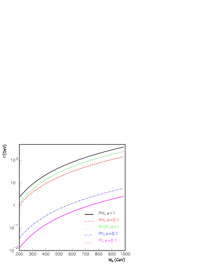
Figure 1: Decay width of $t^{\prime}$ quark depending on its mass for different $V_{t^{\prime}q}$ parametrizations and $\kappa/\Lambda$ values.

III Anomalous Resonant Production of $t^{\prime}$ Quarks

In order to study the resonant production of fourth family quarks, we have implemented the anomalous interaction vertices with the new particles $t^{\prime}$ into CompHEP package comphep (24). In all numerical calculations, the parton distribution functions (PDF) $f_{q}(x,Q^{2})$ and $f_{g}(y,Q^{2})$ are set to the CTEQ6M parametrization R-cteq (25) and the factorization scale $Q^{2}=m_{Q^{\prime}}^{2}$ is used. The total cross section for the process $pp\to W^{+}bX$ is given by

$$\sigma=\int_{\tau_{min}}^{1}d\tau\int_{\tau}^{1}\frac{dx}{x}f_{q}(x,Q^{2})f_{g}(\frac{\tau}{x},Q^{2})\hat{\sigma}(\tau s)$$ (12)

where $\hat{s}=\tau s$ and $\tau_{min}=(m_{V}+m_{q})^{2}/s$; $\hat{\sigma}$ is the partonic cross section for a given process. We consider the production $qg\rightarrow t^{\prime}$ and the decay $t\rightarrow W^{+}b_{j}$. In the generic notation the contributing Feynman diagrams are shown in Fig.2.

Figure 2: Diagrams for the $gq_{i}\to W^{+}q_{j}$ subprocess including $Q^{\prime}qg$ (where $Q^{\prime}\equiv t^{\prime}$) anomalous vertices; $q_{i}$ can be any of the quarks inside the proton, while $q_{j}$ can be any of the quark flavour depending on the charged current interaction. For the $W^{-}\bar{q}_{j}$ final states we may change the direction of the current lines and replace the incoming anti-quarks.

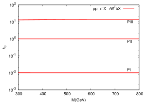
Figure 3: The ratio of the cross sections for different parametrizations normalized to PII, where $\kappa/\Lambda=1$ TeV^-1.

The production cross sections as a function of fourth family quark mass for the different parametrization are shown in Tables 3-5. The ratios of the cross sections for different parametrizations are calculated as $k_{\sigma}\approx 0.01$ for PI and $k_{\sigma}\approx 15$ for PIII with the normalization to PII with $\kappa/\Lambda=1$ TeV^-1, as shown in Fig. 3. For the parametrization PIII we find the $t^{\prime}(\overline{t}^{\prime})$ production cross sections $46.4(11.7)$ pb for $\kappa/\Lambda=0.1$ TeV^-1 and $m_{t^{\prime}}=400$ GeV at $\sqrt{s}=14$ TeV. The $\overline{t}^{\prime}$ production cross section is lower than $t^{\prime}$ production with a factor of 2-8 depending on the considered mass range. The general behaviour of the cross sections depending on the mass is presented in Figs.4-6.

Table 3: Resonance cross sections (pb) and decay widths of $t^{\prime}$ quarks for PI parametrization with $\kappa/\Lambda=1$ TeV^-1 and $\kappa/\Lambda=0.1$ TeV^-1 at $\sqrt{s}=14(10)$ TeV.

	$\kappa/\Lambda=1$ TeV-1			$\kappa/\Lambda=0.1$ TeV-1
$m_{t^{\prime}}$(GeV)	$\sigma(t^{\prime})$	$\sigma(\bar{t^{\prime}})$	$\Gamma_{t^{\prime}}$(GeV)	$\sigma(t^{\prime})$	$\sigma(\bar{t^{\prime}})$	$\Gamma_{t^{\prime}}$(GeV)
300	2.55(0.16)	0.744(1.73x10-3)	5.21	2.53(0.149)	0.693(1.65x10-2)	0.055
400	1.43(6.11x10-2)	0.360(5.16x10-3)	13.74	1.34(0.063)	0.341(5.02x10-3)	0.143
500	0.903(2.68x10-2)	0.198(1.81x10-3)	28.46	0.856(0.027)	0.192(1.77x10-3)	0.296
600	0.608(1.26x10-2)	0.119(7.07x10-4)	50.91	0.582(0.013)	0.114(6.84x10-4)	0.530
700	0.429(6.25x10-3)	0.075(3.0x10-4)	82.59	0.415(0.006)	0.075(2.84x10-4)	0.859
800	0.311(3.2x10-3)	0.049(1.38x10-4)	125.06	0.305(0.003)	0.051(1.22x10-4)	1.30
900	0.232(1.69x10-3)	0.034(6.82x10-5)	179.82	0.217(1.7x10-3)	0.035(5.38x10-5)	1.86
1000	0.174(9.24x10-4)	0.023(3.66x10-5)	248.43	0.178(8.8x10-4)	0.025(2.39x10-5)	2.58

Table 4: Resonance cross sections (pb) and decay widths of $t^{\prime}$ quarks for PII parametrization with $\kappa/\Lambda=1$ TeV^-1and $\kappa/\Lambda=0.1$ TeV^-1 at $\sqrt{s}=14(10)$ TeV.

	$\kappa/\Lambda=1$ TeV-1			$\kappa/\Lambda=0.1$ TeV-1
$m_{t^{\prime}}$(GeV)	$\sigma(t^{\prime})$	$\sigma(\overline{t}^{\prime})$	$\Gamma_{t^{\prime}}$(GeV)	$\sigma(t^{\prime})$	$\sigma(\overline{t}^{\prime})$	$\Gamma_{t^{\prime}}$(GeV)
300	250.92(15.48)	73.30(1.71)	5.29	93.24(5.87)	27.51(0.65)	0.14
400	141.24(6.02)	35.53(0.52)	13.94	55.62(2.44)	14.18(0.21)	0.35
500	88.89(2.64)	19.61(0.18)	28.87	36.26(1.12)	8.18(7.48x10-2)	0.70
600	60.00(1.25)	11.79(6.98x10-2)	51.61	25.16(0.55)	5.06(2.95x10-2)	1.23
700	42.33(0.62)	7.46(2.96x10-2)	83.71	18.14(0.28)	3.29(1.23x10-2)	1.97
800	30.77(0.32)	4.92(1.36x10-2)	126.72	13.45(0.14)	2.23(5.35x10-3)	2.96
900	22.84(0.17)	3.34(6.76x10-3)	182.18	10.22(0.075)	1.55(2.37x10-3)	4.23
1000	17.23(9.1x10-2)	2.32(3.6x10-3)	251.67	7.92(0.039)	1.11(1.07x10-3)	5.82

Table 5: Resonance cross sections (pb) and decay widths of $t^{\prime}$ quarks for PIII parametrization with $\kappa/\Lambda=1$TeV^-1and $\kappa/\Lambda=0.1$ TeV^-1 at $\sqrt{s}=14(10)$ TeV.

	$\kappa/\Lambda=1$ TeV-1			$\kappa/\Lambda=0.1$ TeV-1
$m_{t^{\prime}}$(GeV)	$\sigma(t^{\prime})$	$\sigma(\bar{t^{\prime}})$	$\Gamma_{t^{\prime}}$(GeV)	$\sigma(t^{\prime})$	$\sigma(\bar{t^{\prime}})$	$\Gamma_{t^{\prime}}$(GeV)
300	3272.60(198.72)	946.54(21.92)	9.05	75.28(4.66)	22.03(0.515)	3.89
400	1912.50(79.96)	475.42(6.75)	22.92	46.43(2.00)	11.74(0.169)	9.33
500	1228.70(35.57)	267.17(2.42)	46.46	30.89(0.93)	6.87(6.26x10-2)	18.28
600	835.63(16.85)	161.31(0.96)	82.03	21.60(0.46)	4.28(2.53x10-2)	31.65
700	590.53(8.34)	102.24(0.42)	132.04	15.61(0.23)	2.78(1.1x10-2)	50.30
800	428.19(4.27)	67.04(0.20)	198.88	11.56(0.12)	1.87(4.95x10-3)	75.12
900	315.96(2.26)	45.14(9.96x10-2)	284.95	8.73(0.064)	1.29(2.39x10-3)	106.99
1000	236.33(1.25)	30.94(5.53x10-2)	392.65	6.69(0.035)	0.92(1.23x10-3)	146.79

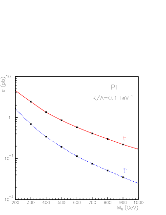
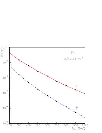
Figure 4: The cross section for the anomalous production of $t^{\prime}$ quarks for PI parametrization and $\kappa/\Lambda=0.1$ TeV^-1. The lines denotes $t^{\prime}(\bar{t^{\prime}})$ followed by the decay $W^{+}b$($W^{-}\bar{b}$) at the center of mass energy 14 TeV (left) and 10 TeV (right).

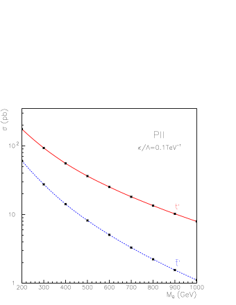
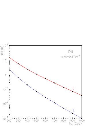
Figure 5: The cross section for the anomalous production of $t^{\prime}$ quarks for PII parametrization and $\kappa/\Lambda=0.1$ TeV^-1. The lines denote $t^{\prime}(\bar{t^{\prime}})$ production followed by the decay $W^{+}b$($W^{-}\bar{b}$) at the center of mass energy 14 TeV (left) and 10 TeV (right).

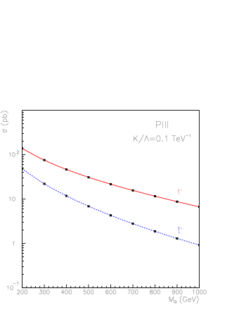
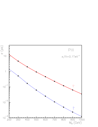
Figure 6: The cross section for the anomalous production of $t^{\prime}$ quarks for PIII parametrization and $\kappa/\Lambda=0.1$ TeV^-1. The lines denote $t^{\prime}(\bar{t^{\prime}})$ production followed by the decay $W^{+}b$($W^{-}\bar{b}$) at the center of mass energy 14 TeV (left) and 10 TeV (right).

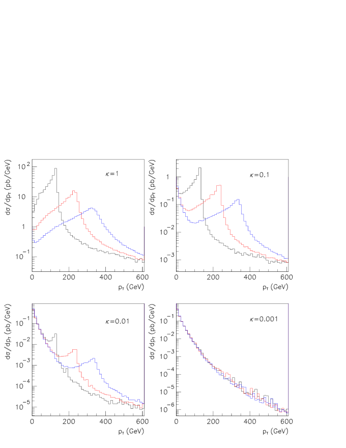
Figure 7: Partonic level $p_{T}$ distributions of $b$ quark from the signal+background process $pp\to W^{+}bX$ at $\sqrt{s}=14$ TeV. The peaks occur around respective half mass values of the $t^{\prime}$ quark masses.

IV Signal and Background

The resonant production mechanisms of the fourth family $t^{\prime}$ quarks depends on the anomalous coupling $\kappa/\Lambda$, while their anomalous decays and charged current decays depend on both these couplings and the $4\times 4$ CKM matrix elements. The signal process $pp\to W^{+}bX$ includes $t^{\prime}$ exchange in the $s$-channel. The $s-$channel contribution to the signal process would manifest itself as resonance around the $t^{\prime}$ mass value in the $W$-boson+jet reconstructed invariant mass. When we consider the leptonic $W$-decays, the $t^{\prime}$ signal search will be $\ell^{+}+b_{jet}+\not E_{T}$, where $\ell=e,\mu$. For the hadronic $W$-decays one would seek the events with one $b$-jet alongside two more jets requiring these to have an invariant mass peak around the $W$-mass. If we consider the dominance of the SM decay mode over the anomalous decay, the $t^{\prime}$ resonant production signal will be

$$\begin{array}[]{cccc}pp\to&t^{\prime}(\bar{t}^{\prime})&X\\ &\hookrightarrow&W^{+(-)}&b_{jet}\\ &\hookrightarrow&W^{+(-)}&j\end{array}$$ (13)

which includes further leptonic or hadronic decays of $W^{+}$boson. In the second and third lines the elements of $4\times 4$ CKM matrix $V_{t^{\prime}b}$ and $V_{t^{\prime}q}$ enter to the decay process for $t^{\prime}$ signal. The cross section for the SM process $pp\to W^{+}bX$ ($pp\to W^{-}\bar{b}X$) is 10.14 pb (9.78 pb) without any cuts at $14$ TeV, and 5.73 pb (5.49 pb) at $10$ TeV. For the cross section estimates, we assume the efficiency for $b$-tagging as $\epsilon_{b}=50\%$, and rejection factors $r_{j}=100$ for light jets, and $r_{c}=10$ for $c(\bar{c})$ quark jets since they are assumed to be mis-tagged as $b$-jets. The $p_{T}$ distributions for both signal and background are given in Fig.7 including the interference terms. Moreover, different background processes contributing to the same final state are presented in Table 6 with various $p_{T}$ cuts. At the center of mass energy $\sqrt{s}=10$ TeV, the background cross sections are calculated as $0.375$ pb (0.354 pb) for $W^{+}b$ ($W^{-}b$), and $2.69\times 10^{3}$ pb (1.88$\times 10^{3}$ pb) for $W^{+}j$ ($W^{-}j$) with $p_{T}^{j}>50$ GeV. The invariant mass distributions of $b\ell\nu$ system at partonic level for different parametrizations are given in Fig. 8. Here, the $W^{+}b$ and $W^{+}j$ backgrounds are included with the assumed efficiencies and acceptance factors. In Fig. 9, we show a density plot of the transverse momentum of the $b$ quark and the invariant mass distribution of $W^{+}b$ system with the $t^{\prime}$ mass constraint.

Table 6: Cross sections for the backgrounds ($W^{\pm}b$ and $W^{\pm}j$) with $p_{T}$ cuts at the center of mass energy $\sqrt{s}=14$ TeV.

Backgrounds	$p_{T}>20$GeV	$p_{T}>50$GeV	$p_{T}>100$GeV
$W^{+}b(W^{-}\overline{b})$	$2.79$($2.71$)	$6.98\times 10^{-1}$($6.71\times 10^{-1}$)	$1.16\times 10^{-1}$($1.09\times 10^{-1}$)
$W^{+}j(W^{-}j)$	$2.22\times 10^{4}$($1.64\times 10^{4}$)	$5.37\times 10^{3}$($3.87\times 10^{3}$)	$1.02\times 10^{3}$($6.92\times 10^{2}$)

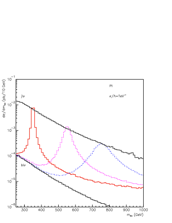
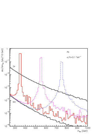
Figure 8: Invariant mass distributions of $b\ell\nu$ system at partonic level for PI (with $p_{T}^{b,j}>100$ GeV), PII (with $p_{T}^{b,j}>50$ GeV), and PIII (with $p_{T}^{b,j}>50$ GeV) parametrizations at $\sqrt{s}=14$ TeV.

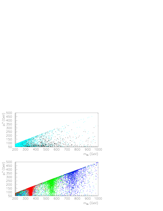
Figure 9: Transverse momentum of the $b$-jet versus $W^{+}b$ invariant mass at $\sqrt{s}=14$ TeV, on the upper panel only the background distribution with $W^{+}b$ (black) and $W^{+}j(b)$ (cyan) events is shown, while on the lower panel both the background and signal distribution with mass of $350$ (red), $550$ (green) and $750$ GeV (blue). Here, the anomalous coupling is taken to be $\kappa/\Lambda=1$ TeV^-1 and the mixing with the fourth family quark $t^{\prime}$ is parametrized as the PII.

V Analysis

At the generator level, we have required a $b$-jet with transverse momentum at least $p_{T}^{b}>50$ GeV for the $W^{+}b$ events. The events generated for each subprocess are mixed using the “mix” script which can be found in the CompHEP package comphep (24), and passed to the PYTHIA pythia64 (26) for further decays and hadronization using the cpyth package belyaev00 (27). After $W$-boson decay and hadronization, the detector effects, such as acceptance and resolution are simulated with PGS4 program conley (28) using generic LHC detector ATLAS99 (29) parameters. This fast simulation includes the most important detector effects, such as $p_{T}$ smearing, $E_{em}$ and $E_{had}$ smearing, energy deposited in towers (granularity) and tag efficiencies of the remaining detector effects such as mis-identifications. More realistic simulation requires the resources of the LHC Collaborations which are beyond the scope of this work. ExRootAnalysis package ExRoot (30) is used to PGS4 data and the output is analysed and histogrammed with the ROOT ROOT (31) macros. Since the cross section for $t^{\prime}\to W^{+}b$ is about five times larger than $\bar{t^{\prime}}\to W^{-}\bar{b}$ cross section, the analysis for the former process has been considered for the remaining of this study.

Typical kinematical distributions are shown in Figs.10 and 11. In the event analysis, the signal ($t^{\prime}\to W^{+}b$, with $\kappa/\Lambda=0.1$ TeV^-1 and $m_{t^{\prime}}=400,500,600$ GeV) and background ($W^{+}b$) are taken into account assuming PIII parametrization. The $W$-boson invariant mass can be reconstructed from its leptonic or hadronic decays. For the leptonic reconstruction case, the criteria is applied to the electrons or muons are: $p_{T}^{\ell}>20$ GeV and $|\eta^{\ell}|<2.5$ whereas for missing transverse energy, the requirement is $\not\!E_{T}>20$ GeV. For the hadronic reconstruction case, we require to find at least 2 jets with $p_{T}^{j}>20$ GeV and $|\eta^{j}|<2.5$. For the reconstruction of the $t^{\prime}$ quark invariant mass, the $b$-tagged jets are required to have $p_{T}^{j_{b}}>50$ GeV and $|\eta^{j_{b}}|<2$ for both cases.

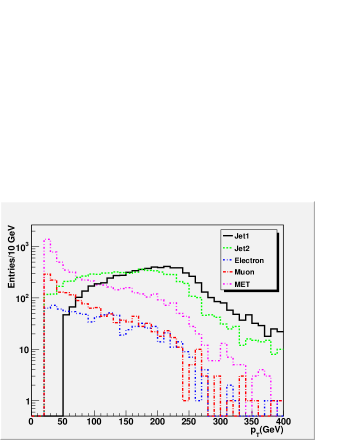
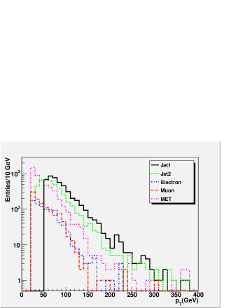
Figure 10: The $p_{T}$ distributions of jets, electrons and muons from the signal ($t^{\prime}\to W^{+}b$) on the left panel, and background ($W^{+}b$) on the right panel shown after detector simulation. The jets are ordered according to the magnitude of their transverse momenta, here we apply the cuts $p_{T}^{j_{1}}>50$ GeV, $p_{T}^{j_{2,3}}>20$ GeV, $p_{T}^{\ell}>20$GeV and $\not\!E_{T}>20$ GeV.

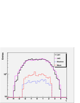
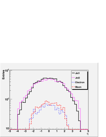
Figure 11: The $\eta$ distributions of jets, electrons, muons from the simulated signal ($t^{\prime}\to W^{+}b$) on the left panel, and background ($W^{+}b$) on the right panel. The jets are ordered according to the magnitude of their $p_{T}$. Typical LHC detectors have the acceptance for $|\eta|<2.5$ when utilization of inner tracker is imposed.

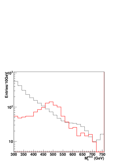
Figure 12: Invariant mass distribution of $b\ell\nu$ system for both signal ($\kappa/\Lambda=0.1$ TeV^-1) and background at $\sqrt{s}=14$ TeV.

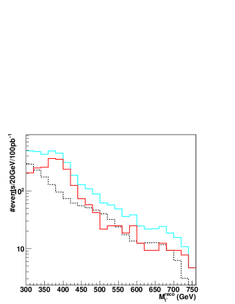
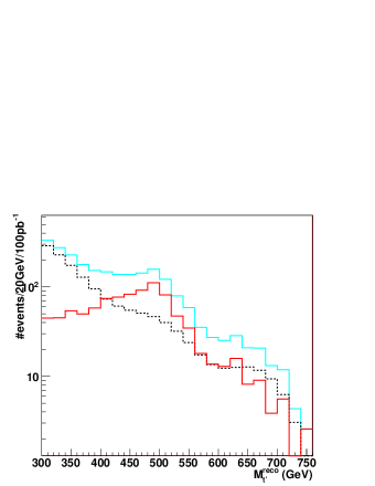
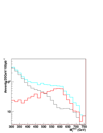
Figure 13: Mass reconstruction of the $t^{\prime}$ signal ($b\ell\nu$) (solid) with $\kappa/\Lambda=0.4$ TeV^-1 for $m_{t^{\prime}}=400$ GeV (upper-left), $m_{t^{\prime}}=500$ GeV (upper-right) and $m_{t^{\prime}}=600$ GeV (lower), and the corresponding background (dashed) at $\sqrt{s}=10$ TeV.

The final results are presented only for the case where the $W$ boson is reconstructed from its leptonic decays. The four momentum vector of the neutrino is calculated from lepton and missing transverse energy assuming a $W$ boson rest mass constraint. The plots for the reconstucted $t^{\prime}$ invariant mass after detector simulation is given in Fig.12 at $\sqrt{s}=14$ TeV and in Fig.13 at $\sqrt{s}=10$ TeV. We include the possible backgrounds contributing to the same final state, and count the signal ($S$) and background ($B$) events in the corresponding mass intervals to calculate the statistical significance (SS) defined as CMSTDR (32) :

$$SS=\sqrt{2\left[(S+B)\ln(1+\frac{S}{B})-S\right]}$$ (14)

In Table 7, the significance calculations are presented for different mass and anomalous coupling values at $\sqrt{s}=10$ TeV. Here, we use the mass bin width $\Delta m=\max(2\Gamma,\delta m)$ to count signal and background events with the mass resolution $\delta m$. The significance increases with $\kappa/\Lambda$ assuming a maximal mixing between the fourth and the third family quarks. The results of this study show that, with early LHC data, one can discover extra up-type quark if there is large anomalous coupling with other up-type quarks.

Table 7: The statistical significance ($SS$) for different masses of $t^{\prime}$ quark, where we take some anomalous parameters in the range ($\kappa=0.1-1.0$) at $\sqrt{s}=10$ TeV and $L_{int}=100$ pb^-1.

$SS$	$m_{t^{\prime}}=400$ GeV	$m_{t^{\prime}}=500$ GeV	$m_{t^{\prime}}=600$ GeV
$\kappa/\Lambda=0.1$ TeV-1	1.91	1.99	2.25
$\kappa/\Lambda=0.2$ TeV-1	6.95	7.19	8.11
$\kappa/\Lambda=0.4$ TeV-1	21.09	21.40	23.44
$\kappa/\Lambda=0.6$ TeV-1	41.97	38.51	38.28
$\kappa/\Lambda=0.8$ TeV-1	55.05	53.05	50.10
$\kappa/\Lambda=1$ TeV-1	65.22	63.14	59.00

VI Conclusion

Anomalous interactions could become significant at tree level processes due to possible large mass of the fourth family quarks. The fourth family $t^{\prime}$ quarks can be produced with large numbers if they have anomalous couplings dominates over the SM chiral interactions. Following the results from the signal significance for $t^{\prime}$ anomalous production the sensitivity to anomalous coupling $\kappa/\Lambda$ can be reached down to $0.1$ TeV^-1in the $b$-jet+lepton+$\not\!E_{T}$ channel at $\sqrt{s}=10$ TeV assuming a maximal parametrization for the extended CKM elements. The LHC experiments can observe the fourth family quarks mostly in pairs and single in the $s$-channel if they have large anomalous couplings to the known quarks. If detected at the LHC experiments the fourth family quarks will change our perpective on the flavor and the mass.

- (1) W.-M. Yao et al., (Particle Data Group) Journal of Physics G 33, 1 (2006).
- (2) P.Q. Hung and M. Sher, Phys. Rev. D 77, 037302 (2008).
- (3) Z. Murdock, S. Nandi and Z. Tavartkiladze, arXiv: 0806.2064 [hep-ph].
- (4) G.D. Kribs, T. Plehn, M. Spannowsky and T.M.P. Tait, Phys. Rev. D 76, 075016 (2007); R. Fok and G.D. Kribs, arXiv: 0803.4207 [hep-h].
- (5) B. Holdom, JHEP 0608, 076 (2006); JHEP 0703, 063 (2007).
- (6) V.A. Novikov, L. B. Okun, A. N. Rozanov and M. I. Vysotsky, JETP Lett. 76, 127 (2002).
- (7) H.-J. He, N. Polonsky, S. Su, Phys. Rev. D 64, 053004 (2001), [hep-ph/0102144].
- (8) V.E. Ozcan, S. Sultansoy and G. Unel, J. Phys. G: Nucl. Part. Phys. 36, 095002 (2009).
- (9) H. Fritzsch, Phys. Lett. B 184, 391 (1987); A. Datta, Pramana 40, L503 (1993); A. Çelikel, A.K. Çiftçi and S. Sultansoy, Phys. Lett. B 342, 257 (1995).
- (10) G. Bregar, M. Breskvar, D. Lukman and N.S. Mankoc Borstnik, arXiv:0708.2846 (hep-ph).
- (11) T. Ibrahim, P. Nath, Phys. Rev. D 78, 075013 (2008).
- (12) B. Holdom, W.S. Hou, T. Hurth, M.L. Mangano, S. Sultansoy, G. Unel, arXiv:0904.4698 [hep-ph].
- (13) CDF Collaboration, CDF Note 8495 (2007).
- (14) CDF Public Note, http://www-cdf.fnal.gov/physics/new/top/2008/tprop/Tprime2.8/public.html.
- (15) N. Cabibbo, Phys. Rev. Lett. 10, 531 (1963); M. Kobayashi and T. Maskawa, Prog. Theor. Phys. 49, 652 (1973).
- (16) V.M. Abazov et al., [D0 Collaboration], arXiv: 0803.0739; CDF Note 8968, [CDF Collaboration], http://www-cdf.fnal.gov/physics/new/top/confNotes/cdf8968_STME_pub.pdf.
- (17) J.A. Herrera, R.H. Benavides, W.A. Ponce, Phys. Rev. D 78, 073008 (2008).
- (18) M. Bobrowski, A. Lenz, J. Riedl and J. Rohrwild, Phys.Rev.D 79, 113006 (2009), arXiv:0902.4883 [hep-ph].
- (19) E. Arik et al., Eur. Phys. J. C 26, 9 (2002); E. Arik et al., Phys. Rev. D 66, 033003 (2002); E. Arik, O. Cakir, S. Sultansoy, Phys. Rev. D 67, 035002 (2003).
- (20) A. K. Ciftci et al., AIP proceedings, 227, (2007).
- (21) O. Cakir et al., Eur. Phys. J. C 56, 537 (2008); arXiv: 0801.0236v2 [hep-ph].
- (22) V.E. Ozcan, S. Sultansoy, G. Unel, Eur.Phys. J. C 57, 621 (2008).
- (23) H. Fritzsch and D. Holtmannspotter, Phys. Lett. B 457, 186 (1999).
- (24) E. Boos et al., [CompHEP Collaboration], Nucl. Instrum. Meth. A534 (2004) 250 (arXiv:hep-ph/0403113).
- (25) J. Pumplin et al., JHEP 0207, 012 (2002) [arXiv:hep-ph/0201195].
- (26) T. Sjostrand et al., JHEP 05, 026 (2006); LU TP 06-13, FERMILAB-PUB-06-052-CD-T, hep-ph/0603175.
- (27) A.S. Belyaev et al., Proc. of ACAT’2000, p.211 (2000), arXiv:hep-ph/0101232.
- (28) J. Conley, Pretty Good Simulation (PGS), http://www.physics.ucdavis.edu/~conway/research/software/pgs/pgs4-general.htm .
- (29) ATLAS Collaboration, CERN/LHCC/94-43; CERN/LHCC/99-14/15 (1999); CMS Collaboration, CMS TDR 8.1, CERN/LHCC 2006-001.
- (30) ExRootAnalysis package for PGS data analysis, http://madgraph.hep.uiuc.edu/Downloads/ExRootAnalysis/ .
- (31) R. Brun and F. Rademakers, ROOT, An object-oriented data analysis framework, v5.22 (2009).
- (32) The CMS Collaboration 2007, J. Phys. G: Nucl. Part. Phys. 34, 995-1579 (2007) .