Classical dimer model with anisotropic interactions on the square lattice
Abstract
We discuss phase transitions and the phase diagram of a classical dimer model with anisotropic interactions defined on a square lattice. For the attractive region, the perturbation of the orientational order parameter introduced by the anisotropy causes the Berezinskii-Kosterlitz-Thouless transitions from a dimer-liquid to columnar phases. According to the discussion by Nomura and Okamoto for a quantum-spin chain system [J. Phys. A 27, 5773 (1994)], we proffer criteria to determine transition points and also universal level-splitting conditions. Subsequently, we perform numerical diagonalization calculations of the nonsymmetric real transfer matrices up to linear dimension specified by and determine the global phase diagram. For the repulsive region, we find the boundary between the dimer-liquid and the strong repulsion phases. Based on the dispersion relation of the one-string motion, which exhibits a two-fold “zero-energy flat band” in the strong repulsion limit, we give an intuitive account for the property of the strong repulsion phase.
pacs:
05.20.-y, 05.50.+qI INTRODUCTION
In the early 1960s, Kasteleyn Kast61 and Temperley and Fisher Temp61 ; Fish61 studied the classical dimer model (DM) defining the statistical-mechanical problem of the covering of a lattice by dimers. They treated the DM on, for example, the square lattice in the thermodynamic limit, and obtained the partition function to give the extensive entropy of an ensemble of dimer configurations. In particular, it was shown that the close-packed model defined on planar lattices can be solved exactly by Pfaffian techniques Kast63 . The properties of these ensembles were studied in subsequent research. For example, those defined on bipartite (non-bipartite) lattices such as the square (triangular) lattice exhibit critical (off-critical) behavior Fish-Step63 ; Fend02 , which are now thought to reflect an existence (absence) of the height representations for the DMs Blot82 ; Blot93 ; Henl97 ; Ardo04 ; Kond95Kond96 . While the relevance of dimers as diatomic molecules adsorbed on a lattice is clear and direct, it can be also related to other degrees of freedom Fish66 . For instance, the zero-temperature Ising-spin antiferromagnet on a triangular (Villain) lattice can be related to the DM on a hexagonal (square) lattice, where each dimer represents an unsatisfied bond of spins Blot82 ; Blot93 ; Vill77 . Also widely known is the string representation whereby dimer systems under a certain condition can be related to loop gases whose configurations are classified by winding numbers (see below) Blot82 ; Blot93 ; Otsu06a . This correspondence has been utilized in discussions of polymer systems Jian07 . More importantly, Rokhsar and Kivelson introduced quantum dimer models (QDMs) to describe the valence-bond physics in quantum Heisenberg antiferromagnets, where the dimer represents a tightly binding singlet pair of quantum spins RK .
These are but a fraction of the examples that show DMs having importance in a wide range of research and drawing attention over the years; in particular, current interest has been mainly focused on exotic phases with topological orders observed in the QDMs Moes01 . More recently, Blunt et al. reported on an adsorption experiment of certain rod-like organic molecules on graphite Blun08 and explained its relevance to the DM on a hexagonal lattice which includes interactions between neighboring dimers Jaco09 . This exhibits the fact that interaction effects in classical dimers are also important from both theoretical and experimental viewpoints Alet05 .
In this paper, we investigate an interacting dimer model (IDM) defined on a square lattice: suppose the lattice constant and let denote the set of lattice sites. Then the following reduced Hamiltonian expresses interactions between two nearest-neighbor dimers:
| (1) |
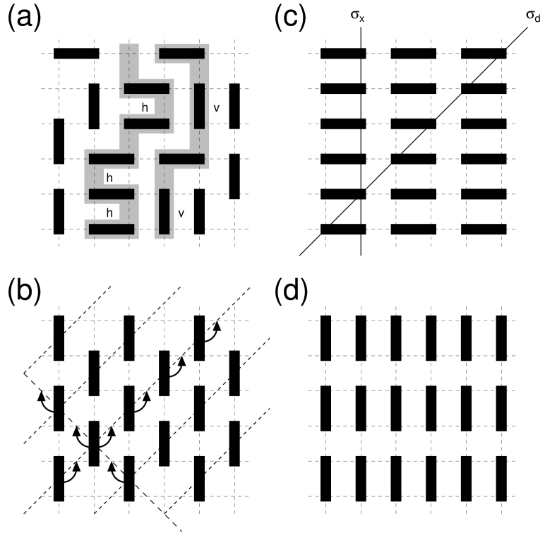
where lattice sites and lattice bonds are denoted, respectively, as and with . We locate the dimer occupation numbers or (binary variables) on the bonds. The first (second) term on the right-hand side of Eq. (1) represents an interaction between parallel horizontal (vertical) dimers [see Fig. 1(a)]. Defining the local Boltzmann weights as
| (2) |
with subscripts on the ’s referring to the corresponding dimer pair, the partition function is then expressible as a summation with respect to the dimer configurations on ,
| (3) |
where [] represents the number of plaquettes with parallel horizontal (vertical) dimers. For large or , an attractive case, a twofold- or a fourfold-degenerate state with columnar order is expected to be stabilized [see examples in Figs. 1(c) and 1(d)]. Meanwhile, for small and , a repulsive case, a highly degenerate phase is stabilized [see an example in Fig. 1(b)]. For the isotropic case , results of some numerical calculations are already available in the literature Alet05 ; Cast07 , but its extension to the anisotropic case is still lacking. Therefore, we shall clarify the global phase diagram and provide evidence corroborating the properties of the phase transitions observed in anisotropically interacting dimers.
According to the effective field theory discussed by Papanikolaou, Luijten, and Fradkin (PLF) Papa07 , one effect absent in the isotropic system is a perturbation by the orientational order parameter; this brings about Berezinskii-Kosterlitz-Thouless (BKT) transitions Bere71 ; Kost73Kost74 . Another effect is a renormalization of the so-called geometric factor, which becomes important in numerical calculations of universal quantities, e.g., the central charge and the scaling dimensions of operators (see below). In such cases, as demonstrated in our own research on an antiferromagnetic Potts model with anisotropic next-nearest-neighbor couplings, the so-called level-spectroscopy analysis Nomu94 ; Nomu95 can provide an effective way to determine phase transition points Otsu06b . For this reason, we shall also employ the same strategy for the present model Otsu05Otsu08 .
For later convenience, we shall briefly explain here the string representation of the DM on . As explicitly explained in Ref. Bogn04 , the transformation of a dimer configuration, e.g., Fig. 1(a), to a string configuration is performed via an XOR operation with reference configuration [Fig. 1(b)]. The XOR operation takes the exclusive OR between occupation (binary) numbers in these two configurations over each bond. Consequently, we obtain strings running in the direction [see the two gray lines in Fig. 1(a)]. Due to the close-packing condition, they have no end points, and thus the string configurations for a system ( is an even number) with periodic boundary conditions can be characterized by winding numbers satisfying . While in the numerical calculation of the transfer matrices we shall employ as a conserved quantity in the row-to-row transfer of configurations, we would rather use a quantity
| (4) |
for convenience in our discussion.
The organization of this paper is as follows: In Sec. II, we review previous research results to give an effective description of the low-energy and long-distance behavior of the IDMs Papa07 . In particular, the operator content of the theory, including expressions of local order parameters and defect operators, and their scaling dimensions are explained in detail. We then provide the conditions to determine the BKT-transition points and clarify some universal relations among excitation levels, which serve as a check of our calculational results. In doing this, a correspondence with a frustrated quantum-spin chain system plays a guiding role. Thus, this correspondence will be emphasized and referred to when appropriate. In Sec. III, we summarize our numerical study and results obtained by the transfer-matrix calculations based on the conformal field theory (CFT) BPZ . First, we demonstrate that the theoretical predictions in Sec. II can be observed precisely via numerical analysis of the excitation spectra. Next, we provide the global phase diagram of interacting dimers, which includes the BKT, the second-order, and the first-order transition lines. Also, in a strong repulsion region, we expect a highly degenerate phase including the staggered state. We calculate the string-number dependence of the free-energy density for the isotropic case. Furthermore, we investigate the “dispersion relation” of the one-string motion, and then based on these data we shall try to give an insight into properties of the strong repulsion phase. The last section, Sec. IV, is devoted to discussion and summary. We also provide our method to evaluate the original BKT transition in the isotropic system. Finally, we compare our data with previous research results.
II THEORY
Continuum field theories offer unified approaches to investigate phase transitions in interacting systems on lattices. They are derived in the scaling limit, while keeping finite. Here is the geometric factor, taking a fixed value, e.g., for isotropic systems on a square (triangular) lattice. However, for anisotropic systems, renormalization of is necessary due to interactions leading to non-universal values. The renormalized can be also related to the velocity of an elementary excitation observed in Tomonaga-Luttinger liquids Hald80 . Thus, disappears from the theoretical description if we properly employ its renormalized value; but as we will see in Sec. III, it becomes rather important in numerical calculations.
According to PLF, the effective description of the IDM takes the form of a sine-Gordon field theory Alet05 . In the present case, its expression is given by the Lagrangian density with
| (5) | |||
| (6) | |||
| (7) |
We denote the course-grained height field in the two-dimensional Euclidean space as , which satisfies a periodicity in height space of () Henl97 . Due to the close-packing of the dimers, the defect operators given in terms of the disorder field dual to are absent from , so that it represents a roughening phase or flat phases of an interface model in three dimensions. The theoretical parameter (the Gaussian coupling) describes the stiffness, and determines the dimensions of the operators on the Gaussian fixed line . In our notation, the vertex operator with electric and magnetic charges is given by whose dimension is
| (8) |
Therefore, () represents the condition that the perturbation () becomes marginal.
To make our discussion more concrete, we introduce the average () and the difference () of the couplings as
| (9) |
where the first (second) subscript refers to the upper (lower) sign. Then, around the non-interacting point, the parameters in are roughly given by
| (10) |
(). We see that the attractive interaction increases , and tends to stabilize the columnar states. Also, in (the orientational order parameter) is proportional to the difference, , while in which is a remnant from the discreteness of the square lattice is almost constant. For , both nonlinear terms are relevant, but they are not competing against each other, so the fourfold-degenerate columnar state stabilized by is only lifted to realize twofold-degenerate columnar states by (see below). Since the BKT transition by was already discussed in the literature Alet05 ; Cast07 , we shall focus our attention on the role of .
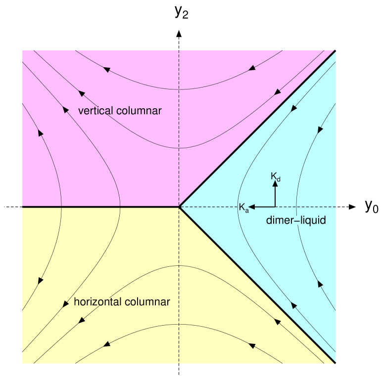
According to the standard argument Poly72 , the renormalization-group (RG) flow diagram of the sine-Gordon model (here is irrelevant) is expressed by the BKT RG equations Bere71 ; Kost73Kost74 ; we depict it by employing the coupling constants and in Fig. 2, where the separatrices separate the dimer-liquid phase from two types of twofold-degenerate columnar phases, namely, the horizontal columnar (HC) state consisting of dimers in the horizontal direction and the vertical columnar (VC) state consisting of dimers in the vertical direction. Now, we can point out that our task to treat the BKT transitions in the IDM can be related to the investigation of the spin- XXZ chain with next-nearest-neighbor interaction because these share the same effective description Nomu94 ; Nomu95 . To specify the relationship, we introduce the following operators:
| (11) | ||||
| (12) | ||||
| (13) |
Here stand for the horizontal and the vertical components of the columnar local order parameter, and take expectation values and ( and ) in the HC (VC) phase; are the defect (or monomer) operators which change the winding numbers classifying dimer configurations. Alternatively, in the quantum-spin chain language, Eqs. (11)–(13) correspond to the Néel, the doublet, and the dimer operators, and give the lowest excitations in the Néel, the spin-liquid, and the dimer phases, respectively (see Table 1). Nomura and Okamoto (NO) provided criteria to determine the BKT-transition points between the spin-liquid and the Néel (or dimer) phases based on one-loop calculations of the scaling dimensions of these operators Giam89 . Therefore, following their argument, we shall discuss procedures to determine the BKT-transition points in our IDM.
| Notations | Operators | Identifications | |||||
|---|---|---|---|---|---|---|---|
| HC (Néel) | 0 | ||||||
| monomer (doublet) | 0 | +1 | |||||
| VC (dimer) | 0 | 0 | +1 | ||||
| Orientational | 0 | ||||||
| Plaquette | 0 |
Consider a system with a finite-strip geometry, viz., a narrow band of width along the direction and infinite length along the direction. The periodic boundary condition is imposed across the width of the strip. The finite-size corrections to the scaling dimensions of the above operators are our key quantities to be evaluated analytically and numerically. Here, we first consider the system near the separatrix where a small parameter can be introduced, so that (). Next, the conformal perturbation calculations of the renormalized scaling dimensions were performed using the sine-Gordon Lagrangian density, for which the results can be summarized as follows:
| (14) | ||||
| (15) | ||||
| (16) |
( is the logarithmic scale length) Giam89 . According to the discussion by NO, we can find the criterion to determine the BKT-transition point (i.e., the level-crossing condition)
| (17) |
and the level-splitting condition as
| (18) |
The latter is one of the universal relations among the excitation levels on the separatrix Zima87 , and enables us to check the consistency of the calculations. Second, we investigate the system near the separatrix ; it proceeds in an analogous way to the above. Writing , we then obtain the dimensions as
| (19) | ||||
| (20) | ||||
| (21) |
Thus, the level-crossing condition needed to determine the transition point is given by
| (22) |
and the level-splitting condition is given by
| (23) |
In analogy to the quantum-spin chain, each level crossing represents an emergence of a SU(2) multiplet structure consisting of the singlet and the triplet states (e.g., and at ). Since these are the low-energy levels in the level-1 SU(2) Wess-Zumino-Witten model Zima87 , our criteria, Eqs. (17) and (22), are natural and also convincing from this viewpoint.
At this stage, two comments are in order about the advantage in using these relations (the level-spectroscopy approach) and the structure of the phase diagram. In Sec. III, we will outline the numerical transfer-matrix calculations performed to obtain the phase diagram. Although it can treat systems with a strip geometry, accessible sizes are strongly restricted to small values, e.g., in our calculations. In the BKT transition, as seen above, the correction terms are typically given by the logarithmic form . If we employ the standard KT criterion such as to determine the transition point, its finite-size estimates include these, and thus exhibit a slow convergence in their extrapolation to the thermodynamical limit. Alternatively, criteria (17) and (22) take the logarithmic corrections into account, so they provide finite-size estimates with fast convergences Nomu95 . Consequently, we can employ the following least-squares-fitting form in extrapolating the finite-size data to the thermodynamic limit :
| (24) |
which includes the term stemming from the irrelevant operators as the leading universal correction Card86a .
The biases from the finite-strip geometry disappear in the limit, and the phase diagram is symmetric with respect to the isotropic line which is one of the inherent properties of the model. Here, we describe how the symmetry of the lattice model is embedded in the sine-Gordon field theory. We shall consider the generators of the -point group: the rotation () and the reflection in the axis () about the original site [see Fig. 1(c)]. As well as coordinate transformations, these bring about the following changes in the height field Alet05 ; Papa07 :
| (25) |
All other elements are obtained from Eq. (25); among them, we shall investigate transformations of the Lagrangian density and the principal operators by reflection about the diagonal line, [see Fig. 1(c)], which shifts the field as
| (26) |
Since the orientational order parameter is odd for , the Lagrangian density transforms as
| (27) |
This indicates a connection between the positive and the negative values of . In addition, the above four operators transform as
| (28) |
Thus, the symmetry operation interchanges the roles of the HC and the VC operators while leaving unchanged the doublet of the monomer excitations. Consequently, as expected, the level-crossing and the level-splitting conditions for , Eqs. (17) and (18), are translated to those for , Eqs. (22) and (23). In Sec. III, we shall provide some numerical data to check this symmetry.
III NUMERICAL CALCULATIONS
Now, consider a system on with the stripe geometry and introduce the transfer matrix connecting nearest-neighbor rows in the direction [see Fig. 1(a)] Alet05 ; Cast07 . As mentioned in Sec. I, the string number in the direction, , is a conserved quantity, which can thus be specified explicitly. We denote the eigenvalues as and their logarithms as ( specifies an excitation level such as those listed in the above). Then, the conformal invariance provides direct expressions of the central charge and the scaling dimension in the critical systems as Blot86 ; Card84
| (29) |
Here, , , and correspond to the ground-state energy, an excitation gap, and a free-energy density, respectively. The ground state is found in the () sector, and the excited levels are also in the sectors specified by the discrete symmetries given in Table 1. In addition, since, independent of the value of , the scaling dimension of a level-1 descendant is equal to 1, it has been utilized to estimate a velocity of elementary excitation in the Tomonaga-Luttinger liquid (see, for example, Nomu94 ). According to their treatment, the effective geometric factor (i.e., inverse velocity) can be also calculated from the descendant level, say , as Otsu06b
| (30) |
The corresponding excitation with small momentum can be found numerically. In calculating and from the excitation gaps via Eq. (29), an estimate of first needs to be obtained. However, it is not necessary in determining the BKT-transition points by Eqs. (17) and (22), because these are homogeneous equations of , and thus the gaps—instead of dimensions—can be used. This is one of the advantages of the level-spectroscopy approach Otsu06b .
In the following, we shall provide our results from numerical calculations for systems up to size . The methodological aspects of transfer-matrix calculations have been well explained in the literature Cast07 . Furthermore, due to the sparse nature of the matrices, we can output all elements to hard disk. Then, using the ARPACK library ARPACK , we can calculate the dominant eigenvalues of the nonsymmetric real matrices.
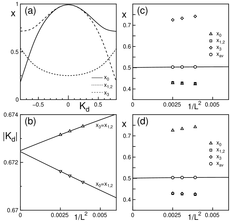
As a demonstration we give the dependence of the scaling dimensions at in Fig. 3(a), where , , and are plotted by solid, dotted, and dashed lines, respectively. While the data are for a system with , we can see the excitation spectra approach quite close to the exact ones at the non-interacting point Fish-Step63 . Furthermore, we find that the HC and the VC excitations interchange their behaviors at , and the former (the latter) shows a level crossing with the doublet excitations at a certain negative (positive) value. According to theoretical predictions (17) and (22), these can provide finite-size estimates of the BKT-transition points to the HC and the VC phases; we shall give some evidence to support our augment. In Fig. 3(b), we exhibit extrapolations of the finite-size estimates to the thermodynamic limit according to Eq. (24). The downward (upward) pointing triangles exhibit values of () at which the crossings between and ( and ) occur in the systems with , 18, and 20. Their extrapolated values strongly agree with each other (i.e., their deviation is within 0.01%), which is the obvious condition to be satisfied. In Figs. 3(c) and 3(d), we plot averaged values, i.e., the left-hand sides (LHSs) of Eqs. (18) and (23), as well as the dimensions at the BKT-transition points estimated in Fig. 3(b). In both cases, the extrapolated values of the averages agree with the theoretical value of , which exhibits universal level splittings due to logarithmic corrections expected at the transition points. These observations show that both our strategy and numerical procedure are valid also for investigations of the IDM Otsu05Otsu08 .
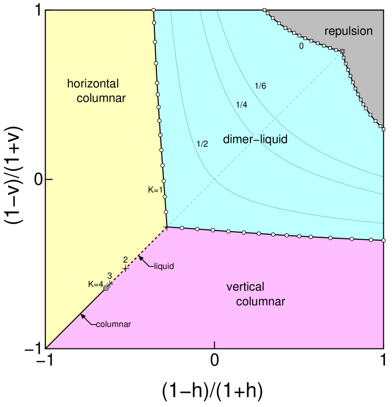
In Fig. 4, we summarize our results of numerical calculations for the global phase diagram of our model (1), in which the diagonal line (the center point) corresponds to the isotropic (noninteracting) system. Due to the fact that the phase diagram is symmetric about the line, it is sufficient to explicitly calculate one side of the whole parameter space; our calculations are thus restricted to the region (i.e., the upper-left triangular area). The open circles with solid lines give the phase boundaries between the dimer-liquid and the columnar phases. In the area apart from the BKT-transition boundaries, we can estimate the Gaussian coupling from the relation . The contour lines of , , and , in addition to the points (plus marks) associated with , , and on the isotropic line are given in the figure. As expected, the dimer-liquid phase spreads over the area satisfying the condition . For , this phase only survives on the isotropic line, but it is eventually terminated by another BKT transition caused by the marginally relevant perturbation. We provide our estimation of the point by our approach (double circle in the figure) although some numerical results were previously available Alet05 ; Cast07 . We shall explain our method and compare our results with these in Sec. IV.
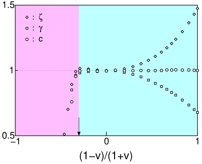
To check the criticality of the dimer-liquid phase, we estimate the central charge along the line by the use of relations (29) and (30). In Fig. 5, we give the dependencies of the effective geometric factor (diamonds), the coefficient of the correction (squares), and their product to estimate (circles). With increasing anisotropy, deviates from the isotropic value of and approaches a certain value around 1.5 in the limit . Simultaneously, declines in value and thus cannot itself give the universal amplitude of the finite-size correction. However, as expected, their product maintains a value within the dimer-liquid phase, and hence the proper normalization using the effective geometric factor is necessary for anisotropic systems. In the attractive region, one finds a point at which the central charge exhibits a steep decrease. We can check that the point is almost on the phase transition boundary to the VC phase (see the vertical arrow), and thus that it is consistent with the level-crossing calculations.
The dimer-liquid region with corresponds to the unstable Gaussian fixed line; the perturbation, except for , brings about second-order phase transitions to the columnar phases. In this case, as , the critical exponent characterizing the diverging correlation length is given by Card86b . To treat this transition, we have performed a finite-size-scaling analysis of the corresponding excitation gaps and have checked that the scaling behavior is very good although we do not provide the data here. In contrast, the liquid phase is absent in the more attractive region, whence the phase transition between the HC and the VC phases becomes first order (the solid line) accompanied by a jump in the phase-locking point from 0 or to or .
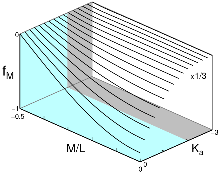
Finally, we discuss the transition to the strong repulsion phase (the upper-right gray-color region) at which the stiffness of the Gaussian model vanishes (see squares with solid lines in Fig. 4). In terms of the height model, this vanishing permits the interface to tilt globally without cost Alet05 ; Frad04 . To get some deeper insight, we shall here focus again on the analogy to a transition observed in the quantum-spin chain. The spin- XXZ chain is solvable Cloi66 ; Yang66 and exhibits criticality for the anisotropy parameter satisfying . This phase is terminated at the SU(2) ferromagnetic point , where there occurs a first-order phase transition accompanied by the vanishing of the Gaussian coupling. At this point, the ground state of the -site chain forms a SU(2) multiplet with total spin and thus possesses degeneracy with respect to the component . This degeneracy is also implied from the following theoretical observation: since the vertex operator corresponding to in Sec. II expresses a -spin flip excitation from the ground state with , the charge in a -site system is restricted to values in . In addition, since the scaling dimension becomes zero in the limit of , at least the corresponding excited levels should degenerate to the ground state to realize the degeneracy Nomu96 ; Naka97 . Returning to our DM where the string number plays a role as a total magnetization, the ground-state energy in each topological sector, , is expected to become independent of . To see this degeneracy, we calculate the -dependent free-energy density . In Fig. 6, we give the results for the isotropic system with . The average of couplings varies within and our estimate of the transition point is (see Sec. IV). One can see that, with decreasing , the free energy tends to show a weaker dependence and, for smaller than roughly the transition point, it becomes almost constant and zero. The above-mentioned degeneracy inferred from the instability of the Gaussian criticality seems to be consistent with this independence. However, there still exists a discrepancy in the degree of degeneracy with the staggered state; we shall discuss this issue for the rest of this section.
It is known that the degeneracy of the staggered state is subextensive, i.e., Cast07 ; Bati04 . This is because, as depicted in Fig. 1(b), the counterclockwise simultaneous rotation of all dimers along a dotted line in the direction can be performed independently of each other—the same holds also for clockwise rotations along the lines in the direction (a dashed line is an example). Thus, if one chooses a certain direction, the staggered state is completely ordered in that direction and completely disordered in the other one. While the problem of how the staggered state is stabilized is quite unclear, we shall try to give an insight based on an analysis of the one-string motion. For convenience, we consider the transfer matrix connecting the next-nearest-neighbor rows, i.e., , so its eigenvalues or their logarithms are squared (i.e., ) or doubled (i.e., ), respectively. We treat two sites as one unit in which four states are included. Then, we can analytically diagonalize the matrix by a Fourier transformation and obtain the -dependence of the energy , i.e., the “dispersion relation” of the one-string motion in the direction. Here, we only show results; the details of how to construct the transfer matrix and also the calculation of eigenvalues in the one-string sector are given in the Appendix. In Fig. 7, for several values of the interactions (isotropic cases), we draw the lower two of four bands. When the eigenvalue becomes a complex number, we take its magnitude in the plot. While the symmetric two-band structure for the non-interacting case [Fig. 7(a)] Kast61 ; Alet05 is deformed by interactions, there is a unique minimum at for finite interaction cases [Figs. 7(b) and 7(c)]. At the same time, as expressed by the dotted lines, complex-conjugate pairs of eigenvalues start to appear near the zone boundary points . And then, in the strong repulsion limit [Fig. 7(d)], we find an emergence of a two-fold degenerate zero-energy flat band. The corresponding eigenvalues are given by , which represents the modulations with wave number in the direction Liebmann . Consequently, our results show dispersionless motion in the and the directions, which precisely reflect the above-mentioned degeneracy, and thus this flat band structure may be a signature of the subextensive degeneracy in the staggered state. If we accept this naive argument, we can conjecture that the staggered state is only realized in the limit. However, our argument is of course at a very speculative level; a full understanding should include also the degeneracy in many-string sectors.

IV DISCUSSIONS and SUMMARY
The isotropic case was discussed in detail in Refs. Alet05 ; Cast07 , where the BKT-transition point driven by and the first-order transition point to the strong repulsion phase were numerically obtained. We have also estimated these transition points (see the double circle and the double square in Fig. 4); in particular, for the former, the above level-spectroscopy approach has been applied. Thus, here we briefly explain our procedure and compare the results. Since the Lagrangian density is analyzed in the region , we focus our attention not on but instead on the following order parameters responsible for the breaking of the rotational symmetry:
| (31) | ||||
| (32) |
While the former is the orientational order parameter, the latter represents the plaquette order Ralk08 which has not been found in classical DMs RK ; Cast07 (the locking points are , , , and ). One then finds that via the transformation and , the Lagrangian density and the operators are reduced to
| (33) |
Therefore, from the discussion in Sec. II, the level-crossing and the level-splitting conditions (17) and (18) are satisfied by the scaling dimensions of these operators, say (here, we have taken the condition into account). Since the half-charge excitations are absent in our system, we employ the condition
| (34) |
to determine the BKT-transition point. The corresponding excitation levels can be found in the sectors specified by their symmetries given in Table 1. We extrapolate the finite-size estimates up to to the thermodynamic limit according to Eq. (24). We then obtain the BKT-transition point as . As we see in Table 2, the agreement with previous results is very good, which indicates that our approach is valid. Similarly, for first-order phase transition, we have estimated the point via condition (see also Ref. Cast07 ) while others have determined this transition from a point of breakdown in the condition . Our result is closer to the estimate of Alet et al. Alet05 although there still exists considerable discrepancy among these estimates. Likewise for instance for phase-separation transitions observed in one-dimensional electron systems, higher-order corrections have been argued to ambiguously affect estimations Naka97 . Thus, we think that the discrepancy in these estimates may reflect their effects.
To summarize, we investigated the anisotropically interacting dimer model on a square lattice. For the attractive case, the orientational-order-parameter perturbation introduced by the anisotropy brings about the BKT transition to the columnar phases. We pointed out the close relationship of our model to a frustrated quantum-spin chain and then found the criteria to determine the transition points. Using these, we performed level-spectroscopy analysis of the eigenvalue structures of the transfer matrices. Numerical results were then summarized as the global phase diagram (Fig. 4), which includes the dimer-liquid, the columnar, and the strong repulsion phases. Furthermore, we checked the level-splitting conditions and evaluated the value of the central charge, which provided solid evidence to confirm the universality of the phase transition. By contrast, for the repulsive case, although we determined the dimer-liquid phase boundary, there exist some points with unclear status within the strong repulsion phase including the staggered state. Based on the dispersion relation of the one-string motion, we gave a possible scenario for the stabilization of the staggered phase. However, although this issue still remains an open question, we now think that the nature of the nonsymmetric real matrix might have relevance to its description Liebmann .
| Criteria | BKT | Criteria | First-order | |||
|---|---|---|---|---|---|---|
| Ref. Alet05 | Order parameters | 1.54 | ||||
| Ref. Cast07 | , , etc. | |||||
| Present | Equation (34) | 1.523 |
ACKNOWLEDGMENT
The author thanks Y. Tanaka, M. Fujimoto, K. Kobayashi, and K. Nomura for stimulating discussions. Most of the computations were performed using the facilities of Information Synergy Center in Tohoku University. This work was supported by Grants-in-Aid from the Japan Society for the Promotion of Science, Scientific Research (C), Contract No. 17540360.
Appendix A A TRANSFER-MATRIX CALCULATION IN ONE-STRING SECTOR
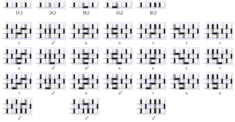
In this appendix, we shall explain how to construct the transfer matrix in the one-string sector and an analytical calculation of eigenvalues by the use of a Fourier transformation. Since a row of the reference configuration given in Fig. 1(b) expresses a string vacuum state, we write it as (see the top left in Fig. 8). For convenience, we treat two sites in the direction as one unit cell which includes four bonds (see squares by dotted blue lines). Then, one-string states can be obtained via replacements of one of unit cells in by four possible dimer configurations. From left to right of the first line in Fig. 8 (except for the vacuum), we call these as , , , and , respectively. Here, the center is supposed to be an th unit cell (). Now, consider transfers of one-string states to those in the next-nearest-neighbor row in the direction. Then, one can find 24 microscopic processes, which are listed in subsequent lines in Fig. 8. For instance, the second line shows seven microscopic processes of transfers from in the first row to states in the third row, and thus exhibits an operation of the transfer matrix, i.e., . Consequently, we can obtain the following recursion relations for the transfers in the one-string sector
| (35) | ||||
| (36) | ||||
| (37) | ||||
| (38) |
where coefficients represent the Boltzmann weights of interactions in the first and the second rows. Next, by the use of the Fourier transformation, we can block-diagonalize the representation of : suppose that
| (39) |
then the -block representation spanned by states , , , is given by a complex nonsymmetric matrix:
| (40) |
where . Hence, the characteristic equation to determine eigenvalues is given by
| (41) |
Since it is invariant under a transformation , a dependence of the eigenvalue structure is even with respect to the point . Meanwhile, in general cases we use a software to evaluate dependences of eigenvalues; in some limiting cases, Eq. (41) becomes simple and permits us to easily manipulate: for instance, for the noninteracting case , two of the four eigenvalues are zero, and the rest is obtained from an equation . It then provides two real bands, as given in Fig. 7(a). In contrast, for the strong repulsion limit , two of the four eigenvalues are zero again, but others are complex values with a modulus of 1, i.e., [see Fig. 7(d)]. An implication of this eigenvalue structure, in particular a correspondence to the degeneracy of states in the IDM is discussed in the last part of Sec. III.
References
- (1) P.W. Kasteleyn, Physica (Amsterdam) 27, 1209 (1961).
- (2) H.N.V. Temperley and M.E. Fisher, Philos. Mag. 6, 1061 (1961).
- (3) M.E. Fisher, Phys. Rev. 124, 1664 (1961).
- (4) P.W. Kasteleyn, J. Math. Phys. 4, 287 (1963).
- (5) M.E. Fisher and J. Stephenson, Phys. Rev. 132, 1411 (1963).
- (6) P. Fendley, R. Moessner, and S.L. Sondhi, Phys. Rev. B 66, 214513 (2002).
- (7) H.W.J. Blöte and H.J. Hilhorst, J. Phys. A: 15, L631 (1982); B. Nienhuis, H.J. Hilhorst, and H.W.J. Blöte, J. Phys. A: 17, 3559 (1984).
- (8) H.W.J. Blöte and M.P. Nightingale, Phys. Rev. B 47, 15046 (1993).
- (9) C.L. Henley, J. Stat. Phys. 89, 483 (1997).
- (10) E. Ardonne, P. Fendley, and E. Fradkin, Ann. Phys. (N.Y.) 310, 493 (2004).
- (11) See also J. Kondev and C.L. Henley, Phys. Rev. B 52, 6628 (1995); Nucl. Phys. B 464, 540 (1996).
- (12) See also M.E. Fisher, J. Math. Phys 7, 1776 (1966).
- (13) J. Villain, J. Phys. C: 10, 1717 (1977).
- (14) H. Otsuka, Y. Okabe, and K. Okunishi, Phys. Rev. E 73, 035105(R) (2006); J. Phys.: Condens. Matter 19, 145236 (2007).
- (15) Y. Jiang and T. Emig, Phys. Rev. B 75, 134413 (2007).
- (16) D.S. Rokhsar and S.A. Kivelson, Phys. Rev. Lett. 61, 2376 (1988).
- (17) For example, R. Moessner and S.L. Sondhi, Phys. Rev. Lett. 86, 1881 (2001).
- (18) M.O. Blunt et al., Science 322, 1077 (2008).
- (19) J.L. Jacobsen and F. Alet, Phys. Rev. Lett. 102, 145702 (2009).
- (20) F. Alet, J.L. Jacobsen, G. Misguich, V. Pasquier, F. Mila, and M. Troyer, Phys. Rev. Lett. 94, 235702 (2005); F. Alet, Y. Ikhlef, J.L. Jacobsen, G. Misguich, and V. Pasquier, Phys. Rev. E 74, 041124 (2006).
- (21) C. Castelnovo, C. Chamon, C. Mudry, and P. Pujol, Ann. Phys. (N.Y.) 322, 903 (2007).
- (22) S. Papanikolaou, E. Luijten, and E. Fradkin, Phys. Rev. B 76, 134514 (2007).
- (23) V.L. Berezinskii, Sov. Phys. JETP 34, 610 (1972).
- (24) J.M. Kosterlitz and J.D. Thouless, J. Phys. C: 6, 1181 (1973); J.M. Kosterlitz, J. Phys. C: 7, 1046 (1974).
- (25) K. Nomura and K. Okamoto, J. Phys. A: 27, 5773 (1994).
- (26) K. Nomura, J. Phys. A: 28, 5451 (1995).
- (27) H. Otsuka, Y. Okabe, and K. Nomura, Phys. Rev. E 74, 011104 (2006).
- (28) See also H. Otsuka, K. Mori, Y. Okabe, and K. Nomura, Phys. Rev. E 72, 046103 (2005); H. Otsuka and K. Nomura, J. Phys. A: Math. Theor. 41, 375001 (2008).
- (29) For example, S. Bogner, T. Emig, A. Taha, and C. Zeng, Phys. Rev. B 69, 104420 (2004).
- (30) A.A. Belavin, A.M. Polyakov, and A.B. Zamolodchikov, Nucl. Phys. B 241, 333 (1984).
- (31) F.D.M. Haldane, Phys. Rev. Lett. 45, 1358 (1980).
- (32) A.M. Polyakov, Sov. Phys. JETP 36, 12 (1973).
- (33) T. Giamarchi and H.J. Schulz, Phys. Rev. B 39, 4620 (1989).
- (34) T. Ziman and H.J. Schulz, Phys. Rev. Lett. 59, 140 (1987), and references therein.
- (35) J.L. Cardy, Nucl. Phys. B 270, 186 (1986).
- (36) J.L. Cardy, J. Phys. A: 17, L385 (1984).
- (37) H.W.J. Blöte, J.L. Cardy, and M.P. Nightingale, Phys. Rev. Lett. 56, 742 (1986); I. Affleck, ibid. 56, 746 (1986).
- (38) R.B. Lehoucq, D.C. Sørensen, and Y. Yang, ARPACK User’s Guide: Solution to Large Scale Eigenvalue Problems with Implicitly Restarted Arnoldi Methods, http://www.caam.rice.edu/software/ARPACK/.
- (39) J.L. Cardy, J. Phys. A: 19, L1093 (1986); J. Phys. A: 20, 5039(E) (1987).
- (40) E. Fradkin, D.A. Huse, R. Moessner, V. Oganesyan, and S.L. Sondhi, Phys. Rev. B 69, 224415 (2004).
- (41) J. Des Cloizeaux and M. Gaudin, J. Math. Phys. 7, 1384 (1966).
- (42) C.N. Yang and C.P. Yang, Phys. Rev. 150, 321 (1966).
- (43) K. Nomura, e-print arXiv:cond-mat/9605070.
- (44) M. Nakamura and K. Nomura, Phys. Rev. B 56, 12840 (1997).
- (45) C.D. Batista and S.A. Trugman, Phys. Rev. Lett. 93, 217202 (2004).
- (46) R. Liebmann, Statistical Mechanics of Periodic Frustrated Ising System, Lecture Notes in Physics Vol. 251 (Springer-Verlag, Berlin, 1986).
- (47) For example, A. Ralko, D. Poilblanc, and R. Moessner, Phys. Rev. Lett. 100, 037201 (2008), and references therein.