Conformations of entangled semiflexible polymers:
entropic trapping and transient non-equilibrium distributions

Abstract

The tube model is a central concept in polymer physics, and allows to reduce the complex many-filament problem of an entangled polymer solution to a single filament description. We investigate the probability distribution function of conformations of confinement tubes and single encaged filaments in entangled semiflexible polymer solution. Computer simulations are developed that mimic the actual dynamics of confined polymers in disordered systems with topological constraints on time scales above local equilibration but well below large scale rearrangement of the network. We observe the statistical distribution of curvatures and compare our results to recent experimental findings. Unexpectedly, the observed distributions show distinctive differences from free polymers even in the absence of excluded volume. Extensive simulations permit to attribute these features to entropic trapping in network void spaces. The transient non-equilibrium distributions are shown to be a generic feature in quenched-disorder systems on intermediate time scales.

1 Introduction

Polymeric networks are not only versatile materials with a large variety of different mechanical properties but also provide interesting model systems for testing concepts of statistical mechanics. Such concepts usually aim to reduce the complicated many-body problem to a tractable single-polymer description as for instance in the well established tube model initiated by de Gennes [1] and Doi and Edwards [2]. This reduction may be complicated by the fact that relevant dynamic processes for an individual polymer, its immediate surroundings and the complete network are each occurring on very different time scales. Furthermore, an additional length scale becomes important if the network is build of semiflexible polymers.

A prominent model system that has recently been thoroughly studied for its relevance to biophysics [3] are filamentous actin (F-actin) solutions. F-actin strands at medium concentrations can form either chemically cross-linked networks in the presence of binding proteins or physically entangled networks for pure solutions with very different elastic properties [4, 5, 6, 7, 8, 9]. These mechanical properties are experimental accessible by means of different rheological methods [4, 10] that mainly probe the collective properties resulting from the interaction of all network constituents on a macroscopic level. The fact that F-actin exceeds most synthetic polymers by length, furthermore permits to observe single network constituents on a microscopic level. For instance, single polymers have been visualized to identify tube-like regions along which filaments reptate [11, 12]. The availability of experimental observation on very different length scales allows to address one of the central questions of polymer physics, how the individual constituents and their behavior collectively determines the macroscopic properties of the polymeric material.

The challenge one is facing in developing a theory for the macroscopic properties of any material that builds on the underlying microscopic physics lies in finding a suitable simplification to describe the large number of network constituents without losing emergent properties. In entangled networks, the only interactions present are of topological nature, as polymers can effortlessly slide past each other but are not allowed to cross. These topological constraints mutually restrict the accessible configuration space of the polymers on intermediate time scales. To account for these entanglement constraints Edwards and de Gennes have introduced the tube model. This surprisingly simple approach successfully reduces the many-polymer problem of a network to a coarse-grained description. The suppression of transverse undulations of a test polymer by the surrounding polymers is mimicked by a hypothetical tube that confines the encaged polymer to a narrow cylindrical pore. This tube follows the average path of the test polymer and its profile is usually described by a harmonic potential. The average strength of this potential and thereby the dimension of the tube is determined by the local density of the network. Semenov derived a scaling law for the dependence of the tube width on monomer concentration by using the assumption that fluctuating filaments explore non-overlapping regions of space [13] and Odijk introduced the deflection length as the length scale between collisions of the probe filament with the tube walls [14]. These scaling laws describing microscopic properties of single polymers in a network are the basis of further theoretical predictions for emerging macroscopic properties. For example, the confinement free energy of the filament inside the tube allows to connect the tube width to mechanical properties of the network [4, 15, 16]. More recently, even nonlinear extension of the standard tube model have been proposed [17].

In this work we go beyond the description of the tube in terms of its average size. We analyze the conformations of tube contours by focussing on the curvature distributions of tube contours and confined polymers. These quantities can provide useful information about equilibration processes and dynamics of confined polymers and are at the foundation of reptation theories [18]. While it is usually assumed that the ensemble of confinement tubes or confined polymers qualitatively shows the same conformation statistics as free polymers, we challenge this assumption.

We will proceed as follows: in Section 2 the system under investigation is defined and all relevant length and time scales are discussed. We identify the characteristic energy distributions in the tube model and present the description in two spatial dimensions. In Section 3 we present our approach to simulate the complete network by a probe filament in a two-dimensional array of obstacles. We pay special attention to the detailed nature of the Monte-Carlo moves used before we present results for the curvature distribution of tubes and filaments and compare them to experiments. As these results seem to disagree with standard concepts of statistical mechanics at a first glance, we devote Section 4 to a thorough analysis of the underlying physics and explain the cause of the surprising results. We corroborate this explanation by further simulations before we concluding in Section 5.

2 Tube Model

We consider entangled solutions of semiflexible polymers where chemical bonds by cross-linking proteins are ruled out. While F-actin is a prominent example of this class of biopolymers and has a strong record of experimental data available, our work is also applicable to other semi-flexible polymer solutions in a comparable regime where a description in the realm of the tube model is justified [19]. As binding by cross-linking proteins is ruled out, the only inter-polymer interactions are topological constraints since network constituents cannot mutually cross each other. The polymers are considered to be mathematical lines as their thickness is negligible [20] and no noteworthy long-ranged attractive or repulsive interactions exists in typical experimental situations. Consequently the system has no excluded volume. In general, F-action solutions are polydisperse with a mean filament length $L\approx 22\mu$m [21]. The detailed length distribution, however, is highly variable for different preparations [22, 23] and we will consider monodispersity in the following. With a persistence length $l_{\rm p}\approx 17\mu$m [24, 25] comparable to its length F-actin is a typical semi-flexible polymer. The polymer’s bending stiffness $\kappa$ is related to the persistence length as $l_{\rm p}=\kappa/k_{\rm B}T$ and each polymer’s configuration ${\bf r}(s)$ is parameterized by the arc length $s$. A free polymer then is described in the worm-like chain model [26, 27] by the Hamiltonian

$$H(\kappa)=\frac{\kappa}{2}\int_{0}^{L}ds\left(\frac{\partial^{2}{\bf r}(s)}{\partial s^{2}}\right)^{2}\;,$$ (1)

where the second derivative of ${\bf r}(s)$ is the local curvature $\mathcal{C}$ at arc-length $s$. As a consequence, the distribution of local curvatures of a free polymer is

$$P(\mathcal{C})\propto\exp\left(-\frac{1}{k_{\rm B}T}H(\kappa,\mathcal{C})\right)\propto\exp\left(-l_{\rm p}\mathcal{C}^{2}\right)$$ (2)

and the resulting Gaussian distribution’s width decreases with increasing persistence length of the polymers.

The density $\nu$ of a network of these polymers is given by the number of polymers of length $L$ per unit volume. At a concentration of $c=0.5$ mg/ml corresponding to $\nu\approx 1\mu m^{-3}$ [28] the average distance to the next neighbor is given by the mesh mesh size $\xi\approx(\nu L)^{-1/2}\approx 0.2\mu$m and therefore much smaller then polymer length and persistence length, $\xi\ll l_{\rm p}$. Due to this ratio of length scales it is guaranteed, that a specific polymer will not deviate far from its average contour and it is highly unlikely to fold back onto itself. Thus it is feasible to model the combined effect of all neighboring filaments of an arbitrary probe polymer by a hypothetical tube potential. The tube potential has a harmonic profile as observed in experiments and simulations [29, 30]. Due to the disorder in the network the tube diameter and thus the local strength of the tube potential vary along the contour [31]. The tube is conventionally described by a potential strength $\gamma(s)$ that is parameterized by the arc length $s$ along the tube backbone or tube contour given by the potential’s minimum in space. If we denote this tube backbone by ${\bf r}_{0}(s)$, the resulting energy becomes the sum of the bending energy of the polymer and its confinement by a harmonic potential around the tube backbone

$$H(\gamma,\kappa)=\int_{0}^{L}ds\left[\frac{\kappa}{2}\left(\frac{\partial^{2}{\bf r}(s)}{\partial s^{2}}\right)^{2}+\frac{\gamma}{2}\left[{\bf r}(s)-{\bf r}_{0}(s)\right]^{2}\right]\;.$$ (3)

In contrast to a free polymer this equation does not allow to infer a simple distribution of curvatures as in Eq. 2 because the second term causes an additional dependence on the tube contour. This term causes a confinement around the minimum of the potential that is given by the tube backbone as explained above. If for instance the backbone is already strongly bend and the confinement potential is sufficiently strong, high curvatures are more likely than for a free polymer. Obviously the distribution of curvatures of any probe polymer sensitively depends on the actual form of the tube to which it is confined. Furthermore, the conformations of the tube backbone is itself a statistically distributed quantity. Finally, it is important to state that a tube is well-defined only up to some intermediate time scale. Therefore, in networks of non cross-linked polymers the tube model cannot be used as an equilibrium concept without further thought. The confinement tube is defined as the space accessible to an encaged polymer in an environment of neighboring filaments before large scale reconstruction of the network changes this environment. The tube picture is thus a valid description as soon as the polymer experiences topological interaction with its neighbors and as long as these are not remodelled by large scale dynamics. The first time scale can be estimated from dynamic light scattering as the point were a cross-over from free filament to restricted dynamics sets in at about 10 ms [32]. An estimate for the time scale of remodelling can be obtained from the time it takes the probe filament to leave its initial tube. For unstabilized actin filaments this process is dominated by treadmilling occurring at an approximate rate of 2 $\mu m$ per hour [33]. Stabilized actin filaments where treadmilling is abolished by phalloidin can only reptate out of their tubes at much slower rates. Reptation rates in this case have been estimated from experiments [34, 35] to be as long as several days for a 10 $\mu m$ long filament.

As explained above, a well established scaling law for the average tube diameter has been derived by Semenov. Recently, also theories providing absolute values have been proposed [30, 36] and confirmed experimentally [31]. In analyzing experimental data it is important to keep in mind that fluorescence microscopy only provides an observation of an effectively two-dimensional focal plane. For the tube diameter this implies that only fluctuations in one Cartesian component are measured. In the focal plane the system can be considered as a probe filament surrounded by fluctuating point obstacles that represent the cuts of neighboring polymers through the the plane of observation as depicted in Fig. 1.

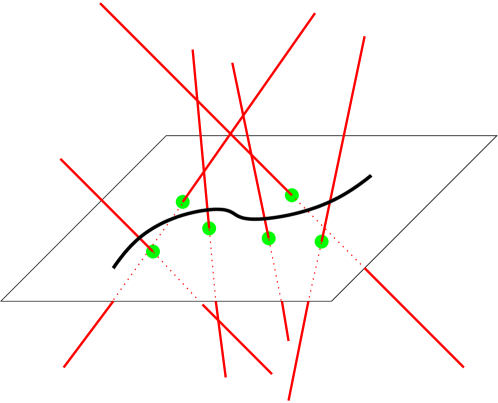
Figure 1: In a two-dimensional cut through the network, as e.g. in the focal plane of a microscope, neighboring polymers reduce to point-like obstacles.

3 Monte-Carlo Simulations

Motivated by this point of view, we have developed a Monte-Carlo simulation with the standard Hastings-Metropolis algorithm [37] to observe curvature distribution functions of a single probe filament in a two-dimensional plane of point-like obstacles. This does not only provide ready comparability with experiments, but is also a valid simplification of the three-dimensional problem since transverse undulations in different components can be assumed to be independent. As the surrounding network constituents are very thin and nearly straight due to their large persistence length it is justified to represent them by point-like obstacles. Those obstacles undergo themselves transversal fluctuations that have to exhibit on average the same characteristics as the fluctuations of the probe filament for reasons of self-consistency. As the latter were found to be harmonic, the same must hold for the in-plane fluctuations of an obstacle polymer that cuts perpendicularly through the simulation plane. If the cutting angle is tilted the harmonic profile is distorted corresponding to different fluctuation strength for the two in-plane components. While the average tube diameter must equal the fluctuation strength averaged over all obstacles, the distribution of these two quantities may be broad [30]. It was found, however, that the simulation results are rather insensitive to these parameters. The simulation is thus an adequate and self-consistent description of the physical problem of a entangled network of semi-flexible polymers, if the parameters obstacle density $\rho$ and obstacle fluctuation potential strength $\gamma$ are chosen to represent the corresponding polymer density $\nu$ and resulting tube diameter $L_{\perp}$. These parameters have been shown [30] to be:

$$\rho=\frac{2}{\pi}\nu L\;,\qquad\gamma\approx 4.18(\nu L)^{3/5}l_{p}^{1/5}\;.$$ (4)

The probe filament of length $L$ is initially placed in a straight configuration onto the plane of observation and is represented by a sequence of $N$ connected segments $i$ with orientation ${\bf t}_{i}$. Due to inextensibility the segments are of fixed length $L/N$. In a first step the filament is allowed to relax on the plane without the presence of any obstacles. The relaxation is performed with respect to an Hamiltonian :

$$H(\{{\bf t}_{i}\})=-J\sum_{i=1}^{N-1}{\bf t}_{i}{\bf t}_{i+1}\;,$$ (5)

where in two dimensions the relation between persistence length and $J$ is given as $l_{p}/L=-[N\ln(I_{1}(J)/I_{0}(J))]^{-1}$ with $I_{n}$ the modified Bessel functions of first kind [38]. After equilibration with respect to the Hamiltonian (5) the probe filament features the bending distribution of a free polymer. Now the obstacle fluctuation centers $p^{0}_{j}$ are fixed to random positions of the simulation plane. While these centers remain fixed for the course of the simulation, the positions of the point obstacles $p_{j}$ themselves - initially placed at $p_{j}=p^{0}_{j}$ - are allowed to move in a harmonic potential $U=\frac{1}{2}\gamma_{j}(p_{j}-p^{0}_{j})^{2}$. Their motion is not only governed by this potential but also by the constraint that they must not cross the probe filament and they remain on that side of the probe filament where they had been initially placed . Naturally, the same constraint also holds for the probe filament where every move, that would lead to a configuration where an obstacle point had switched sides, is rejected. While the motion of the point obstacles is straightforward, we will discuss the moves of the probe filament in more detail in the following section.

3.1 Dynamic Trial Moves

In the construction of trial moves our intention has been to find a set of moves that mimics the underlying local dynamics in the physical system as closely as possible. To this end it is of particular importance to keep the relevant time scales in mind. Therefore, our choice of moves describes the effect of the underlying physical forces and dynamics on a probe filament for times well below large scale rearrangement of the network. These have to include transverse undulations, exploration of void spaces along the contour and small-scale reptation and breathing, while the effects of large scale reptation like annihilation and creation of obstacle points remain impossible. In the following, we will thoroughly explain the moves used in our Monte-Carlo simulations. As shown below, the resulting data for conformations and distribution functions sensitively depends on their nature.

We use four different moves, that change the polymer configuration on different levels ranging from local change in only one tangent up to a global manipulation of the complete polymer contour. The classical random pivot move (see Fig. 2 (a)) chooses a random tangent AB and rotates it by a small random angle. This changes the two bending angles at A and B but leaves all other angles invariant. However, all positions along the polymer contour are modified - predominantly in a direction transverse to the contour. Another move employed is a flip move (see Fig. 2 (b)). Here two beads A and B separated by a random number of segments are picked and all points are mirrored along the axis connecting A and B. This can be seen as the two-dimensional analogon to a crankshaft move. The flip move leaves the ends of the polymer unaffected. These two rather common moves are known to effectively explore the available phase space of free polymers or even of polymers in pore-like potentials. However, they lack the ability to mimic the motion of a polymer into the void spaces between obstacles along the walls of the hypothetical tube.

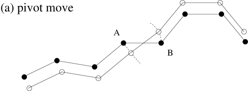
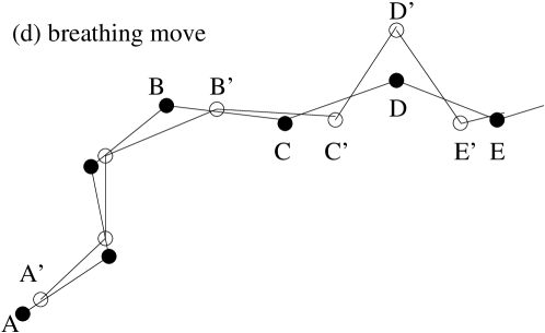
Figure 2: The different moves performed during the simulations. Full circles denote the original positions and open circles the new configuration: (a) The pivot move changes two angles and all positions. (b) The flip move changes all angles and positions between A and B. (c) The “trade-off” move changes the curvature of the section CE in a trade-off with the adjacent section to both sides (only l.h.s section AC depicted here). (d) The “breathing” move changes all positions and angles and axially moves the polymer’s ends.

To this end we use novel moves that are depicted in Fig. 2 (c) and (d). They simulate the exploration of a local void space, i.e. a part where the “tube” formed by the fluctuating obstacles is rather large. Due to the negligible longitudinal extensibility of semi-flexible polymers the motion of the polymer into this void space is obviously possible only if the other parts of the polymer are retracted or straightened out. Let us first introduce the move that performs the latter and is illustrated in 2 (c). The additional length that is needed to enable the protrusion into a void space is obtained from undulations in adjacent parts of the polymer. A stronger bending in one part is made possible by weaker bending in other parts and we therefore choose the label “trade-off” move. Specifically, the move is conducted by randomly choosing two points C and E, that are separated by an even distance of segments (in our simulations we apply two different moves where this distance is either two or four). This is the region of the polymer that should explore the void space. Furthermore, to the left and right of this region two more points are chosen that enclose the regions that will be straightened out to compensate for the contour length drawn into the void. At the left hand site this is for example point A that is separated from C by an again even number of tangents (in our simulations two to ten). We restrict our illustration to the left hand site, but the same process also applies to a comparable region on the right hand side that is not shown. In addition to a random number $R_{\mathrm{loc}}$ to choose the location of the section $CE$ along the contour, we draw another random number $R_{\delta}$ that quantifies the extend of change in bending. Our goal is now to construct a algorithm that straightens out the region AC in order to enable the region CE to realize a stronger bending. In a first step the vector AB is prolonged to AB’ by adding a random small amount $\delta$. The new point between A and B is chosen in a way to keep tangent length conserved. In a next step B’C is prolonged to B’C’ by adding the same $\delta$ and so on. The same process is performed on the right hand side tail. This results in two points C’ and E’ that are separated by a smaller distance than the original pair C and E. The remaining section in between is now fitted in under the precondition of length conservation. After construction the new configuration is checked for violation of the topological constraints and bending energy.

Naturally, also a backward move has to be possible that pushes back the region CE into a lesser bend conformation by creating or enhancing undulations in the region AC. This process is performed if the random distance $\delta$ is negative and is achieved in the following way. We proceed in a reverse fashion by first choosing points B’ and C’ and reducing their distance by $\delta$. The same is performed along the tails until the final point of the region AC is reached. The result is a distance between points C and E that is now larger than the original distance between the points C’ and E’ and thus a section CE that is pulled back from the void to a straighter configuration and enhanced undulations along the left and right tails. Note that exclusive performance of this move will leave the polymer ends unchanged. In combination with the other moves however, it allows for a longitudinal motion of the ends by effectively manipulating the undulations along the encaged contour.

After having constructed a novel trial move for a Monte-Carlo simulation it is of crucial importance to check if it guarantees a conversion of the simulation to equilibrium. While it is know that this can be achieved by the balance condition [39] it is usually more convenient to check the stricter condition of detailed balance [40]. It requires that in equilibrium for every pair of configurations $m$ and $n$ the moves from $m$ to $n$ given by $P^{0}_{m}P^{\mathrm{move}}_{m\to n}P^{\mathrm{acc}}_{m\to n}$ equal the number of reverse moves $P^{0}_{n}P^{\mathrm{move}}_{n\to m}P^{\mathrm{acc}}_{n\to m}$. Here, $P^{0}$ is the Boltzmann weight of a configuration, $P^{\mathrm{move}}$ is the a priori probability to select a certain move and $P^{\mathrm{acc}}$ is the probability that this move is accepted. For the move introduced above, every move is characterized by the two random numbers $R_{\mathrm{loc}}$ and $R_{\delta}$ and its backward move is simply obtained by changing the sign of $\delta$. Consequently, the a priori probabilities of every move and its corresponding backward move cancel. The acceptance probability is zero for both move and backward move if topological constraints are violated. If the topology is conserved the move is accepted according to change in bending energy and thus according to the ratio of Boltzmann factors and consequently the condition of detailed balance is guaranteed.

Finally the fourth trial move, a global “breathing” move, mimics a global retraction of the polymer along its contour to enable the exploration of void spaces. This move causes a pronounced axial motion of the polymer ends and is schematically depicted in Fig. 2 (d). Again, by a random number $R_{\mathrm{loc}}$ a section CE is randomly chosen in which the local curvature is to be manipulated. Either the bending of CE is enhanced resulting in a global retraction of the remaining tail sections of the polymer to the left and right hand side of CE, or the bending of CE is diminished which is achieved by pushing out the remaining sections. As the manipulation of the tail sections is always to occur along the polymer’s contour, bending of CE causes axial motion of both ends towards the polymer’s center and straightening out of CE causes end motion away from the center. In detail the new configuration in the former case is constructed by choosing a new C’ by reducing the distance between C and E by a small random $\delta$ as above. B’ is then found at that point where a radius $L/N$ intersects with the old polymer contour. All other points are chosen accordingly proceeding towards the polymer’s ends. The back move is obtained by extending the section CE by $\delta$ and fixing the direction of the tail segments by demanding that they pass through the joint points of the old contour . Thereby, again the exact backward move to any given move is simply obtained by inverting the sign of $\delta$. Consequently, the same reasoning as above also proves detailed balance.

We validated this particular choice of Monte-Carlo moves in a simulation of a single free polymer, where we compared our observations to established results of the bending distribution of free polymers, tangent-tangent correlation function and end-to-end distribution function [41]. All results presented in the following were obtained as a combined ensemble and time average. Ensemble averaging was performed over a large number of initial obstacle fluctuation center distributions. Additionally, for every initial obstacle distribution several initial distributions for the probe filament were chosen. This can also be seen as averaging over different topologies. After initial equilibration, observables were monitored and averaged for the remainder of the simulation time thereby averaging over all statistically allowed configurations in a fixed topology.

3.2 Simulation Results

In a first step we characterized the conformation of the confinement tubes - a quantity that is also accessible by fluorescence microscopy and therefore allows for a comparison to experimental data. To this end we determine the tube contour, i.e. the backbone of the area to which the probe filament is confined, by averaging over the contour of the probe polymer in its cage of point obstacles over the evolution. From the resulting contour we determine a curvature distribution $P(\mathcal{C})$, where the curvature is defined by locally fitting a parabola with $y=\mathcal{C}x^{2}/2$ to the contour. The distribution obtained after averaging over initial conditions is shown in Fig. 3.

Figure 3: Curvature distribution of confinement tube contours as obtained from Monte-Carlo simulations (dashed line) and from experiments (full line) [31]. The curvature distribution of a free filament obtained by the same simulation algorithm is plotted for comparison (dotted line). The inset shows the same data in a semilogarithmic plot.

We compare our data to measurements that were obtained by fluorescence microscopy [31] of in vitro solutions of rhodamine-phalloidin labeled F-actin on a minute time scale . The good agreement of the data is evidence that our simulation approach provides a reliable representation of the physical system under consideration.

In comparison to the curvature distribution obtained by the same algorithm for free filaments, two distinctive differences emerge. While the free filament distribution has to be Gaussian as explained in Eq. 2, the distribution function of the tube contours features a pronounced exponential tail. As an exponential decays much slower as a Gaussian towards high values, this signifies that highly bend filaments are much more frequent. Also for the occurrence of small curvatures a strong increase in probability compared to the case of free filaments can be observed. The form of the distribution, however, remains Gaussian, making the difference rather quantitative. It is obvious that relative to free filaments, probability is both shifted to smaller and larger curvatures at the cost of medium curvatures. This reflects the visual observation that tube contours are on average straighter than free polymers but also feature distinctive strongly bend sections. The first feature, i.e. the increase of small local bendings, obviously results only from the averaging procedure carried out in determining the tube backbone. The averaging over all topologically allowed polymer conformations within the tube integrates out fluctuations of small wavelength (small radii of curvature) to obtain a larger radius of curvature for the coarse-grained tube contour. The increase in highly bend filaments on the exponential tail of the curvature distribution is far less obvious. To avoid the complications of coarse-graining related to the tube contour, we turn to a different observable. The curvature distribution of the encaged filament itself is not as easily accessible to experiments and thus does not allow for verification, but it allows a direct comparison to free filaments. In particular, this is the case for solutions with negligible excluded volume, where the bending distribution obtained by standard statistical mechanics should be identical.

We recorded snapshots of the probe polymer during the evolution and analyzed these for their curvature as explained above to obtain the curvature distribution of confined filaments depicted in Fig. 4.

Figure 4: Curvature distribution of encaged filaments obtained from Monte-Carlo simulations (solid line) compared to the distribution of a free filament (dotted line). The inset shows the same data in a semilogarithmic plot.

Now the distribution at small and medium curvatures remains largely unaffected as compared to free filaments. However, the pronounced exponential tail at high curvatures is still observed. These features were observed for networks composed of polymers of different persistence length. At a first glance this behavior seems to contradict general concepts of statistical mechanics that do not predict any effect of topological constraints in a system without excluded volume. We will explain in the following how this conflict is resolved.

4 Thermodynamic Interpretation

As discussed in Sec. 2, the probe filament is confined to its tube during the time window that is relevant to many biological processes and that is the observation frame for most experimental measurements as well. Clearly, our simulations have also been tailored to represent this intermediate time scale as point-obstacle centers are fixed and large scale reptation is beyond simulation time. Therefore all observations made on this time scale are crucially influenced by the tube’s properties and we will discuss the implications for the obtained averages and trace back the results for the deviation of the curvature distribution from the free filament case. To this end, we will first of all recapitulate some general notions on standard thermodynamic averaging, then pinpoint differences to averaging procedures in the tube model and finally present additional simulations to corroborate our findings. To facilitate our discussion we restrict ourselves in the following to the case of a probe filament in a two-dimensional array of fixed point-like obstacles. This simplified system has the same general characteristic as a polymer confined to a tube in a network but considerably less degrees of freedom.

4.1 Ensemble Average - Time Average

If one is faced with the problem to calculate averages for a statistical system there are in general two different possibilities: an ensemble average and a time average that will yield the same result if the system is ergodic. An ensemble average in the system under consideration could be realized by drawing a large number of allowed configuration of the complete network and weighing them by the corresponding Boltzmann factor. As there is no interaction between polymer and obstacles and in the absence of excluded volume no initial configuration can be rejected due to hard-core exclusion, the only contribution to the Boltzmann factor is the bending term of the worm-like chain (Eq. 1) and the average obtained has to equal the case of free polymers. Due to the absence of excluded volume the polymer is not able to see the obstacles and any probe polymer inserted into the network has zero chance of overlap or rejection. The concept of a time average, on the contrary, would be to start from one initial probe polymer configuration and monitor the following time evolution. As soon as the probe polymer has explored every point in phase space, the obtained average equals the ensemble average. In the obstacle system however, the time to fulfill this requirement is exceedingly long. Points that might be very close to each other in phase space can be very far apart in terms of transition time. This is due to the fact that the topological constraints that the obstacles impose, partition the phase space into a multitude of areas that are not directly connected. Consequently, the probe filament can only traverse a point obstacle by completely reptating back and forth. Due to the immense number of different topologies and the slow reptation time scale (see Sec. 2) a complete time average is not only out of the scope of simulations and experiments but also irrelevant to biological processes.

4.2 Partitioned Averaging

It can now be tried to substitute the infeasible sampling of phase space by means of reptation of a single test polymer by a large number of samples with different initial conditions. Here, initial configurations of the test polymer are drawn from the free polymer distribution and randomly placed into the obstacle network. Different topologies emerge as the same obstacle could be at the left or right of the test polymer. Starting from these initial conditions the polymer’s configurations are now sampled employing a Markovian Monte-Carlo dynamics respecting the topological constraints imposed by the neighboring obstacles. Such a procedure corresponds to a partitioning of phase space into sections with‘different topologies”, i.e. areas that are not directly connected. One could therefore argue, that an average containing all possible topologies should also hold the same results as a complete time average or averaging of a free polymer. However, this argument can only be valid if the partitions of phase space are disjunct. Otherwise, if these partitions overlap, the averaging procedure will put a higher or smaller weight on some microstates. The curvature distribution obtained by the experimental and simulational averaging procedure can thus only be expected to equal the free polymer case, if it is guaranteed that during the observation time the topology and hence the partitioning of phase space remains unaltered for every test polymer. Processes that can modify the topology are for instance reptation or “breathing” of the polymer. One mutual feature of these processes is that they cause motion of the polymer ends tangentially along the contour. Therefore obstacles can switch their topology with respect to the test polymer, e.g. an obstacle initially left of the test polymer can end up being on the right side after the polymer’s end has moved back and forth. The requirement of strict disjunct partitioning of phase space would thus essentially amount to the constraint of keeping the polymer’s ends fixed which is evidently not the case in the actual physical system.

We, therefore, conclude that the polymer dynamics inside the confinement tubes are metrically transitive due to their characteristic features as breathing and reptation that change the topology in the network array. The topological partitioning is thus not maintained under the dynamic evolution. Therefore the resulting averages and distribution functions have not necessarily to equal the corresponding results for free polymers. This holds on intermediate time scales before large scale reptation sets in, which are the time scales of experimental observation. In the long time limit, however, when the single polymers of the ensemble have been able to explore larger parts of the phase space beyond their confinement tubes, free filament distributions should be recovered. Consequently, the observed non-equilibrium distribution functions do not violate thermodynamic requirements as they are transient. However, the time needed for total equilibration is so long, that it is not reached on any applicable time scale.

After we have shown, how transient non-equilibrium distribution functions can arise on intermediate time scales even in the absence of excluded volume, we will use additional simulations to clarify the physical origins of highly bend filaments.

Figure 5: A typical network configuration where transient entropic trapping occurs when the probe filament explores a void space by high bending thereby realizing an entropic gain.

4.3 Additional Simulations - Entropic Trapping

To this end we have conducted further simulations of the simplified system of fixed obstacles. Note, that this work does not apply to a network of F-Actin as represented by the simulations with self-consistently fluctuating obstacles. It merely serves as an model system for our considerations on the averaging procedures. First of all, we have checked if a system where dynamics have chosen to be metrically intransitive faithfully reproduces the distribution functions of free filaments. This was achieved by running simulations where the filament’s Monte-Carlo moves are restricted to “flip” and “trade-off” moves. This choice ensures that the polymer’s ends do not move axially. As obstacles remain fixed, it is guaranteed that the topological partitioning cannot change. The resulting distribution function indeed reproduces the case of free filaments (see Fig. 6 (top)). Furthermore, we have identified the physical origins of the highly bend parts of the test polymer. It turns out that high curvatures occur always at local initial topologies where a test polymer can protrude into a large void space in the obstacle array (see Fig. 5). The initial conformation of the test polymer already has a curvature that facilitates a further bending into a large void part in the network. Hereby the system realizes a higher entropy by bending harder than the equilibrium curvature distribution. These events are rare but they dominate the tail of the curvature distribution. Apparently, the polymer is trapped in these entropically favorable configurations on the time scale of observation. This behavior bears some similarity to “entropic trapping” observed for flexible polymers in random environments [42, 43, 44, 45]. Note in particular, that these conformations also result in a pulling back of the polymer ends and thus a change of phase space partition. Hence, this observation does not only clarify the physical cause of high bendings but also proves according to the argumentation above that a curvature distribution different from the free polymer distribution does not violate statistical mechanics.

Furthermore, we have investigated how these special conformations are realized as a function of the fluctuation amplitude of the obstacles. For both self-consistently fluctuating and immobile obstacles an exponential tail is visible in the curvature distribution. This is also the case for obstacles fluctuating with a higher amplitude as in the self-consistent case. The weight on the high curvature tail is highest for immobile obstacles and decreases with increasing fluctuation amplitude. This is consistent with the explanation for the high bendings provided above. As the effective size of void spaces is diminished with larger obstacle fluctuation the effect decreases. In the limiting case of very large fluctuations network obstacles become delocalized, the system is reduced to a gas and the curvature distribution of a free polymer will be recovered.

Figure 6: Curvature distributions compared to free filaments (dotted line): (top) metrically intransitive system with fixed ends (solid line), (bottom) probe filament in obstacles of different fluctuation strength.

5 Conclusion

We have investigated the curvature distribution functions in entangled networks of semiflexible polymers. To this end we developed an approach to simulate single probe filaments in an entangled network of semi-flexible polymers by a self-consistent reduction to a two-dimensional setup corresponding e.g. to the focal plane of a microscope to allow for comparison for experimental data. This Monte-Carlo simulations were particularly designed to mimic the real polymer dynamics on intermediate time scales by allowing for an effective exploration of network void spaces by breathing and short scale reptation. The simulations provide data on curvature distributions for tube contours that agree well with fluorescence microscope measurements on F-actin solutions [31]. Furthermore, they permit to observe curvature distributions of single confined filaments. These distributions feature an unexpectedly high weight on highly bend filaments that is traced back to transient entropic trapping in network void spaces. The fact that the equilibrium distribution of free polymers is not recovered even in the absence of excluded volume, is shown to be an immanent feature of the polymer dynamics in a disordered environment on intermediate time scales below large scale reptation. The fact that this regime is best described by the tube model - a non-equilibrium concept - explains that a treatment in terms of equilibrium thermodynamics is inappropriate. Consequently, the observation of transient non-equilibrium distribution functions is a generic effect observed for all measurements on time scales both relevant to experiments and feasible for simulations. These findings provide insight into the conformation of confined polymers and can e.g. prove useful for further analysis of reptation or emerging collective macroscopic properties.

Acknowledgement: We thank R. Merkel and his group for fruitful cooperation and J.U. Sommer for discussions on “entropic trapping”. We acknowledge support from the DFG through SFB 486, from the German Excellence Initiative via the NIM program and from the Elite Network of Bavaria through the NBT program.

References

- [1] P. G. de Gennes. Scaling Concepts in Polymer Physics. Cornell University Press, Ithaca, NY, 1979.
- [2] M. Doi and S. F. Edwards. The Theory of Polymer Dynamics. Clarendon Press, Oxford, 1986.
- [3] A. R. Bausch and K. Kroy. Nature Physics, 2(231), 2006.
- [4] B. Hinner, M. Tempel, E. Sackmann, K. Kroy, and E. Frey. Phys. Rev. Lett., 81:2614, 1998.
- [5] D. A. Head, A. J. Levine, and F. C. MacKintosh. Phys. Rev. Lett., 91:108102, 2003.
- [6] J. Wilhelm and E. Frey. Phys. Rev. Lett., 91:108103, 2003.
- [7] M. L. Gardel, J. H. Shin, F. C. MacKintosh, L. Mahadevan, P. Matsudaira, and D. A. Weitz. Science, 304:1301, 2004.
- [8] C. Heussinger and E. Frey. Phys. Rev. Lett., 97:105501, 2006.
- [9] B. Wagner, R. Tharmann, I. Haase, M. Fischer, and A. R. Bausch. Proc. Nat. Acad. Sci., 103:13974, 2006.
- [10] F. Amblard, A. C. Maggs, B. Yurke, A. N. Pargellis, and S. Leibler. Phys. Rev. Lett., 77:4470, 1996.
- [11] T. T. Perkins, D. E. Smith, and S. Chu. Science, 264:819, 1994.
- [12] J. Käs, H. Strey, and E. Sackmann. Nature, 368:226, 94.
- [13] A. N. Semenov. J. Chem. Soc. Faraday. Trans., 82:317, 1986.
- [14] T. Odijk. Macromolecules, 16:1340, 1983.
- [15] F. C. MacKintosh, J. Käs, and P. A. Janmey. Phys. Rev. Lett., 75:4425, 1995.
- [16] H. Isambert and A. C. Maggs. Macromolecules, 29:1036, 1996.
- [17] P. Fernandez, S. Grosser, and K. Kroy. Soft Matter, 5:2047, 2009.
- [18] M. Doi. Journal of Polymer Science, 73:93, 1985.
- [19] F. Wagner, G. Lattanzi, and E. Frey. Phys. Rev. E, 75:050902, 2007.
- [20] K. C. Holmes, D. Popp, W. Gebhard, and W. Kabsch. Nature, 347:44, 1990.
- [21] S. Kaufmann, J. Käs, W. H. Goldmann, and G. Isenberg. FEBS Lett., 314:203, 1992.
- [22] J. Käs, H. Strey, J. X. Tang, D. Finger, R. Ezzell, E. Sackmann, and P. A. Janmey. Biophys. J., 70:609, 1996.
- [23] M. Kawamura and K. Maruyama. Journal of Biochemisty, 67(3):437, 1970.
- [24] F. Gittes, B. Mickey, J. Nettleton, and J. Howard. J. Cell Biol., 120:923, 1993.
- [25] L. Le Goff, O. Hallatschek, E. Frey, and F. Amblard. Phys. Rev. Lett., 89:258101, 2002.
- [26] O. Kratky and G. Porod. Rec. Trav. Chim., 68:1106, 1949.
- [27] N. Saito, K. Takahashi, and Y. Yunoki. J. Phys. Soc. Jpn., 22:219, 1967.
- [28] C. F. Schmidt, M. Baermann, G.Isenberg, and E. Sackmann. Macromolecules, 22:3638, 1989.
- [29] M. A. Dichtl and E. Sackmann. New. J. Phys., 1:18.1, 1999.
- [30] H. Hinsch, J. Wilhelm, and E. Frey. E. Phys. J. E, 24:35, 2007.
- [31] M. Romanowska, H. Hinsch, N. Kirchgessner, M. Giesen, M. Degawa, B. Hoffmann, E.Frey, and R.Merkel. Europhys. Lett., 86:26003, 2009.
- [32] C. Semmrich, T. Storz, J. Glaser, R. Merkel, A. R. Bausch, and K. Kroy. Proc. Natl. Acad. Sci. USA, 104:20199, 2007.
- [33] N. Selve and A. Wegner. Journal of Molecular Biology, 187:627, 1986.
- [34] M. A. Dichtl and E. Sackmann. Proc. Natl. Acad. Sci. USA, 99:6533, 2002.
- [35] M. Keller, R. Tharmann, M. A. Dichtl, A. R. Bausch, and E. Sackmann. Phil. Trans. Roy. Soc. London A, 361:699, 2003.
- [36] D. C. Morse. Phys. Rev. E, 63:031502, 2001.
- [37] W. K. Hastings. Biometrika, 57:97, 1970.
- [38] M. E. Fisher. American Journal of Physics, 32:343, 1964.
- [39] Vasilios I. Manousiouthakis and Michael W. Deem. J. Chem. Phys., 110(6):2753, 1999.
- [40] D. Frenkel and B. Smit. Understanding Molecular Simulations. Academic Press, San Diego, 1996.
- [41] J. Wilhelm and E. Frey. Phys. Rev. Lett., 77:2581, 1996.
- [42] A. Baumgartner and M. Muthukumar. J. Chem. Phys., 87:3082, 1987.
- [43] M. E. Cates and R. C. Ball. J. Phys. France, 49:2009, 1988.
- [44] S.F. Edwards and M. Muthukumar. J. Chem. Phys., 89:2435, 1988.
- [45] J. U. Sommer and A. Blumen. Phys. Rev. Lett., 79(3):439, 1997.