Search for a light Higgs boson at BABAR

Abstract

We search for evidence of a light Higgs boson (${A^{0}}$) in the radiative decays of the narrow $\mathchar 28935\relax{(3S)}$ resonance: $\mathchar 28935\relax{(3S)}\rightarrow\gamma{A^{0}}$, where $A^{0}\rightarrow\mathrm{invisible}$ or ${A^{0}}\rightarrow\mu^{+}\mu^{-}$. Such an object appears in extensions of the Standard Model, where a light $C\!P$-odd Higgs boson naturally couples strongly to $b$-quarks. We find no evidence for such processes in a sample of $122\times 10^{6}$ $\mathchar 28935\relax(3S)$ decays collected by the BABAR collaboration at the PEP-II B-factory, and set 90% C.L. upper limits on the product of the branching fractions $\mathcal{B}(\mathchar 28935\relax(3S)\rightarrow\gamma A^{0})\times\mathcal{B}(A^{0}\rightarrow\mathrm{invisible})$ at $(0.7-31)\times 10^{-6}$ in the mass range $m_{A^{0}}\leq 7.8$ GeV, and on the product $\mathcal{B}(\mathchar 28935\relax(3S)\rightarrow\gamma A^{0})\times\mathcal{B}(A^{0}\rightarrow\mu^{+}\mu^{-})$ at $(0.25-5.2)\times 10^{-6}$ in the mass range $0.212\leq m_{A^{0}}\leq 9.3$ GeV. We also set a limit on the dimuon branching fraction of the recently discovered $\eta_{b}$ meson ${\cal B}(\eta_{b}\rightarrow\mu^{+}\mu^{-})<0.8\%$ at 90% C.L. The results are preliminary.

1 INTRODUCTION

The concept of mass is one of the most intuitive ideas in physics since it is present in everyday human experience. Yet the fundamental nature of mass remains one of the greatest mysteries in physics. The Higgs mechanism is a theoretically appealing way to account for the different masses of elementary particles [1]. The Higgs mechanism implies the existence of at least one new particle called the Higgs boson, which is the only Standard Model (SM) [2] particle yet to be observed. If it is found, its discovery will have a profound effect on our fundamental understanding of matter. A single Standard Model Higgs boson is required to be heavy, with the mass constrained by direct searches to $m_{H}>114.4$ GeV [3] and $m_{H}\neq 170$ GeV [4], and by precision electroweak measurements to $m_{H}=129^{+74}_{-49}$ GeV [5].

The Standard Model and the simplest electroweak symmetry breaking scenario suffer from quadratic divergences in the radiative corrections to the mass parameter of the Higgs potential. Several theories beyond the Standard Model that regulate these divergences have been proposed. Supersymmetry [6] is one such model; however, in its simplest form (the Minimal Supersymmetric Standard Model, MSSM) questions of parameter fine-tuning and “naturalness” of the Higgs mass scale remain.

Theoretical efforts to solve unattractive features of MSSM often result in models that introduce additional Higgs fields, with one of them naturally light. For instance, the Next-to-Minimal Supersymmetric Standard Model (NMSSM) [7] introduces a singlet Higgs field. A linear combination of this singlet state with a member of the electroweak doublet produces a $C\!P$-odd Higgs state $A^{0}$ whose mass is not required to be large. Direct searches typically constrain $m_{A^{0}}$ to be below $2m_{b}$ [8] making it accessible to decays of $\mathchar 28935\relax$ resonances. An ideal place to search for such $C\!P$-odd Higgs would be $\mathchar 28935\relax\rightarrow\gamma{A^{0}}$, as originally proposed by Wilczek [9]. A study of the NMSSM parameter space [10] predicts the branching fraction to this final state to be as high as $10^{-4}$.

Other new physics models, motivated by astrophysical observations, predict similar light states. One recent example [11] proposes a light axion-like pseudoscalar boson $a$ decaying predominantly to leptons and predicts the branching fraction ${\cal B}(\mathchar 28935\relax\rightarrow\gamma\ a)$ to be between $10^{-6}$–$10^{-5}$ [11]. Empirical motivation for a light Higgs search comes from the HyperCP experiment [12]. HyperCP observed three anomalous events in the $\mathchar 28934\relax\rightarrow p\mu^{+}\mu^{-}$ final state, that have been interpreted as a light scalar with mass of $214.3$ $\mathrm{\,Me\kern-1.00006ptV}$ decaying into a pair of muons [13]. The large datasets available at BABAR allow us to place stringent constraints on such models.

If a light scalar ${A^{0}}$ exists, the pattern of its decays would depend on its mass. In dark matter inspired scenarios, $A^{0}\rightarrow\mathrm{invisible}$ decays could be dominant. For low masses $m_{A^{0}}<2m_{\tau}$, relevant for the axion [11] and HyperCP [12] interpretations, the dominant decay mode should be ${A^{0}}\rightarrow\mu^{+}\mu^{-}$. Significantly above the tau-pair threshold, ${A^{0}}\rightarrow\tau^{+}\tau^{-}$ would dominate, and the hadronic decays may also be significant.

Preliminary results from search for invisible Higgs decays are described in Ref. [14]. This analysis [15] searches for the radiative production of Higgs in $\mathchar 28935\relax{(3S)}$ decays, which subsequently decays into muons:

$$\mathchar 28935\relax{(3S)}\rightarrow\gamma{A^{0}};\ {A^{0}}\rightarrow\mu^{+}\mu^{-}$$

The current best limit on the branching fraction $\mathcal{B}(\mathchar 28935\relax\rightarrow\gamma{A^{0}})$ with ${A^{0}}\rightarrow\mu^{+}\mu^{-}$ comes from a measurement by the CLEO collaboration on $\mathchar 28935\relax(1S)$ [16]. The quoted limits on ${\cal B}(\mathchar 28935\relax{(1S)}\rightarrow\gamma{A^{0}})\times{\cal B}({A^{0}}\rightarrow\mu^{+}\mu^{-})$ are in the range (1-20)$\times 10^{-6}$ for $m_{A^{0}}<3.6$ $\mathrm{\,Ge\kern-1.00006ptV}$. There are currently no competitive measurements at the higher-mass $\mathchar 28935\relax$ resonances or for the values of $m_{A^{0}}$ above the $\tau\tau$ threshold.

In the following, we describe a search for a resonance in the dimuon invariant mass distribution for fully reconstructed final state $\mathchar 28935\relax{(3S)}\rightarrow\gamma(\mu^{+}\mu^{-})$. We assume that the decay width of the resonance is negligibly small compared to experimental resolution, as expected [11, 17] for $m_{A^{0}}$ sufficiently far from the mass of the $\eta_{b}$ [18]. We also assume that the resonance is a scalar (or pseudo-scalar) particle; while significance of any peak does not depend on this assumption, the signal efficiency and, therefore, the extracted branching fractions are computed for a spin-0 particle. In addition, following the recent discovery of the $\eta_{b}$ meson in $\mathchar 28935\relax{(3S)}$ decays [18], we look for the leptonic decay of the $\eta_{b}$ through the chain $\mathchar 28935\relax{(3S)}\rightarrow\gamma\eta_{b}$, $\eta_{b}\rightarrow\mu^{+}\mu^{-}$. If the recently discovered state is the conventional quark-antiquark $\eta_{b}$ meson, its leptonic width is expected to be negligible. Thus, setting a limit on the dimuon branching fraction sheds some light on the nature of the recently discovered state. We assume $\Gamma(\eta_{b})=10$ MeV, which is expected in most theoretical models and is consistent with BABAR results [18].

2 THE BABAR DETECTOR AND DATASET

We search for two-body transitions $\mathchar 28935\relax(3S)\rightarrow\gamma{A^{0}}$, followed by the decay $A^{0}\rightarrow\mathrm{invisible}$ [14] or ${A^{0}}\rightarrow\mu^{+}\mu^{-}$ [15] in a sample of $(121.8\pm 1.2)\times 10^{6}$ $\mathchar 28935\relax(3S)$ decays collected with the BABAR detector at the PEP-II asymmetric-energy $e^{+}e^{-}$ collider at the Stanford Linear Accelerator Center. The data were collected at the nominal center-of-mass (CM) energy $E_{\mathrm{cm}}=10.355$ GeV. The CM frame was boosted relative to the detector approximately along the detector’s magnetic field axis by $\beta_{z}=0.469$.

We use a sample of $78.5\,\mathrm{fb}^{-1}$ accumulated on $\mathchar 28935\relax{(4S)}$ resonance ($\mathchar 28935\relax{(4S)}$ sample) for studies of the continuum backgrounds; since $\mathchar 28935\relax{(4S)}$ is three orders of magnitude broader than $\mathchar 28935\relax{(3S)}$, the branching fraction $\mathchar 28935\relax{(4S)}\rightarrow\gamma{A^{0}}$ is expected to be negligible. For characterization of the background events and selection optimization we also use a sample of $2.4\,\mathrm{fb}^{-1}$ collected $30$ MeV below the $\mathchar 28935\relax{(3S)}$ resonance.

The BABAR detector is described in detail elsewhere [19]. We use the GEANT4 [20] software to simulate interactions of particles traversing the BABAR detector, taking into account the varying detector conditions and beam backgrounds.

3 EVENT SELECTION FOR $A^{0}\rightarrow\mu^{+}\mu^{-}$ DECAYS

We select events with exactly two oppositely-charged tracks and a single energetic photon with a CM energy $E^{*}_{\gamma}\geq 0.5$ $\mathrm{\,Ge\kern-1.00006ptV}$. We allow other photons to be present in the event as long as their CM energies are below $0.5$ $\mathrm{\,Ge\kern-1.00006ptV}$. We assign a muon mass hypothesis to the two tracks (henceforth referred to as muon candidates), and require that they form a geometric vertex with the $\chi^{2}_{\mathrm{vtx}}<20$ (for 1 degree of freedom), displaced transversely by at most $2$ cm from the nominal location of the $e^{+}e^{-}$ interaction region. We perform a kinematic fit to the $\mathchar 28935\relax{(3S)}$ candidate formed from the two muon candidates and the energetic photon, constraining the CM energy of the $\mathchar 28935\relax{(3S)}$ candidate, within the beam energy spread, to the total beam energy $\sqrt{s}$. We also assume that the $\mathchar 28935\relax{(3S)}$ candidate originates from the interaction region. The kinematic fit improves the invariant mass resolution of the muon pair. We place a requirement on the kinematic fit $\chi^{2}_{\mathchar 28935\relax{(3S)}}<39$ (for 6 degrees of freedom), which corresponds to the probability to reject good kinematic fits of less than $10^{-6}$. The kinematic fit $\chi^{2}$, together with a requirement that the total mass of the $\mathchar 28935\relax{(3S)}$ candidate is within 2 $\mathrm{\,Ge\kern-1.00006ptV}$ of $\sqrt{s}$, suppresses background events with more than two muons and a photon in the final state, such as cascade decays $\mathchar 28935\relax{(3S)}\rightarrow\gamma\chi_{b}(2P)\rightarrow\gamma\gamma\mathchar 28935\relax{(1S)}\rightarrow\gamma\gamma\mu^{+}\mu^{-}$ etc. We further require that the momentum of the dimuon candidate ${A^{0}}$ and the photon direction are back-to-back in the CM frame to within $0.07$ radians, and select events in which the cosine of the angle between the muon direction and ${A^{0}}$ direction in the center of mass of ${A^{0}}$ is less than $0.88$. We reject events in which neither muon candidate is positively identified in the muon chamber.

The kinematic selection described above is highly efficient for signal events. After the selection, the backgrounds are dominated by two types of QED processes: “continuum” $e^{+}e^{-}\rightarrow\gamma\mu^{+}\mu^{-}$ events in which a photon is emitted in the initial or final state, and the initial-state radiation (ISR) production of the vector mesons $J/\psi$, $\psi(2S)$, and $\mathchar 28935\relax{(1S)}$, which subsequently decay into muon pairs. In order to suppress contributions from ISR-produced $\rho^{0}\rightarrow\pi^{+}\pi^{-}$ and $\phi\rightarrow K^{+}K^{-}$ final states in which a pion or a kaon is misidentified as a muon or decays (e.g. through $K^{+}\rightarrow\mu^{+}\nu_{\mu}$), we require that both muons are positively identified when we look for ${A^{0}}$ candidates in the range $m_{A^{0}}<1.05$ $\mathrm{\,Ge\kern-1.00006ptV}$. Finally, when selecting candidate events in the $\eta_{b}$ mass region $m_{\mu\mu}\sim 9.39$ $\mathrm{\,Ge\kern-1.00006ptV}$, we require that no secondary photon above a CM energy of $E_{2}^{*}=0.08$ $\mathrm{\,Ge\kern-1.00006ptV}$ is present in the event; this requirement suppresses decay chains $\mathchar 28935\relax{(3S)}\rightarrow\gamma_{2}\chi_{b}(2S)\rightarrow\gamma_{1}\gamma_{2}\mathchar 28935\relax{(1S)}$, in which the photon $\gamma_{2}$ has a typical CM energy of 100 MeV.

We use Monte Carlo samples generated at 20 values of $m_{A^{0}}$ over a broad range $0.212<m_{A^{0}}\leq 9.5$ GeV of possible $A^{0}$ masses to measure selection efficiency for the signal events. The efficiency varies between 24-44%, depending on the dimuon invariant mass.

4 EXTRACTION OF SIGNAL YIELDS FOR $A^{0}\rightarrow\mu^{+}\mu^{-}$ DECAYS

The invariant mass spectrum for the selected candidates in the $\mathchar 28935\relax{(3S)}$ dataset is shown in Fig. 1 (left). We extract the yield of signal events as a function of the assumed mass $m_{A^{0}}$ in the interval $0.212\leq m_{A^{0}}\leq 9.3$ GeV by performing a series of unbinned extended maximum likelihood fits to the distribution of the “reduced mass”

$$m_{R}=\sqrt{m_{\mu\mu}^{2}-4m_{\mu}^{2}}\ .$$ (1)

The choice of this variable is motivated by the distribution of the continuum background from $e^{+}e^{-}\rightarrow\gamma\mu^{+}\mu^{-}$, which is a smooth function of $m_{R}$ across the entire range of interest, in particular, the region near the kinematic threshold $m_{\mu\mu}\approx 2m_{\mu}$ ($m_{R}\approx 0$). Each fit is performed over a small range of $m_{R}$ around the value expected for a particular $m_{A^{0}}$. We use the $\mathchar 28935\relax{(4S)}$ sample to determine the probability density functions (PDFs) for the continuum background in each fit window, which agree within statistical uncertainties with Monte Carlo simulations. We use a threshold (hyperbolic) function to describe the background below $m_{R}<0.23$ $\mathrm{\,Ge\kern-1.00006ptV}$; its parameters are fixed to the values determined from the fits to the $\mathchar 28935\relax{(4S)}$ dataset. Elsewhere the background is well described in each limited $m_{R}$ range by a first-order ($m_{R}<9.3$ GeV) or second-order ($m_{R}>9.3$ GeV) polynomial.

The signal PDF is described by a sum of two Crystal Ball functions [21] with tail parameters on either side of the maximum. The signal PDFs are centered around the expected values of $m_{R}=\sqrt{m^{2}_{{A^{0}}}-4m_{\mu}^{2}}$ and have the typical resolution of $2-10$ MeV, which increases monotonically with $m_{A^{0}}$. We determine the PDF as a function of $m_{A^{0}}$ using a set of high-statistics simulated samples of signal events, and we interpolate PDF parameters and signal efficiency values linearly between simulated points. We determine the uncertainty in the PDF parameters by comparing the distributions of the simulated and reconstructed $e^{+}e^{-}\rightarrow\gamma_{\mathrm{ISR}}J/\psi$, $J/\psi\rightarrow\mu^{+}\mu^{-}$ events.

Known resonances, such as ${J\mskip-3.0mu/\mskip-2.0mu\psi\mskip 2.0mu}$, $\psi(2S)$, and $\mathchar 28935\relax{(1S)}$, are present in our sample in specific intervals of $m_{R}$, and constitute peaking background. We include these contributions in the fit where appropriate, and describe the shape of the resonances using the same functional form as for the signal, a sum of two Crystal Ball functions, with parameters determined from the dedicated MC samples. We do not search for ${A^{0}}$ signal in the immediate vicinity of ${J\mskip-3.0mu/\mskip-2.0mu\psi\mskip 2.0mu}$ and $\psi(2S)$, ignoring the region of $\approx\pm 40$ MeV around ${J\mskip-3.0mu/\mskip-2.0mu\psi\mskip 2.0mu}$ (approximately $\pm 5\sigma$) and $\approx\pm 25$ MeV ($\approx\pm 3\sigma$) around $\psi(2S)$.

For each assumed value of $m_{A^{0}}$, we perform a likelihood fit to the $m_{R}$ distribution under the following conditions:

• $0.212\leq m_{A^{0}}<0.5$ GeV: we use a fixed interval $0.01<m_{R}<0.55$ GeV. The fits are done in 2 MeV steps in $m_{A^{0}}$. We use a threshold function to describe the combinatorial background PDF below $m_{R}<0.23$ $\mathrm{\,Ge\kern-1.00006ptV}$, and constrain it to the shape determined from the large $\mathchar 28935\relax{(4S)}$ dataset. For $m_{R}>0.23$ $\mathrm{\,Ge\kern-1.00006ptV}$, we describe the background by a first-order Chebyshev polynomial and float its shape, while requiring continuity at $m_{R}=0.23$ $\mathrm{\,Ge\kern-1.00006ptV}$. Signal and background yields are free parameters in the fit.

• $0.5\leq m_{A^{0}}<1.05$ GeV: we use sliding intervals $\mu-0.2<m_{R}<\mu+0.1$ GeV (where $\mu$ is the mean of the signal distribution of $m_{R}$). We perform fits in 3 MeV steps in $m_{A^{0}}$. First-order polynomial coefficient of the background PDF, signal and background yields are free parameters in the fit.

• $1.05\leq m_{A^{0}}<2.9$ GeV: we use sliding intervals $\mu-0.2<m_{R}<\mu+0.1$ GeV and perform fits in 5 MeV steps in $m_{A^{0}}$. First-order polynomial coefficient of the background PDF, signal and background yields are free parameters in the fit.

• $2.9\leq m_{A^{0}}\leq 3.055$ GeV and $3.135\leq m_{A^{0}}\leq 3.395$ GeV: we use a fixed interval $2.7<m_{R}<3.5$ GeV; 5 MeV steps in $m_{A^{0}}$. First-order polynomial coefficient of the background PDF, signal, $J/\psi$, and background yields are free parameters in the fit.

• $3.4\leq m_{A^{0}}<3.55$ GeV: we use sliding intervals $\mu-0.2<m_{R}<\mu+0.1$ GeV and perform fits in 5 MeV steps in $m_{A^{0}}$. First-order polynomial coefficient of the background PDF, signal and background yields are free parameters in the fit.

• $3.55\leq m_{A^{0}}\leq 3.66$ GeV and $3.71\leq m_{A^{0}}<4.0$ GeV: we use fixed interval $3.35<m_{R}<4.1$ GeV; 5 MeV steps in $m_{A^{0}}$. First-order polynomial coefficient of the background PDF, signal, $\psi(2S)$, and background yields are free parameters in the fit.

• $4.0\leq m_{A^{0}}<9.3$ GeV: we use sliding intervals $\mu-0.2<m_{R}<\mu+0.1$ GeV; 5 MeV steps in $m_{A^{0}}$. First-order polynomial coefficient of the background PDF, signal and background yields are free parameters in the fit.

• $\eta_{b}$ region ($m_{\eta_{b}}=9.390$ GeV): we use a fixed interval $9.2<m_{R}<9.6$ GeV. We constrain the contribution from $e^{+}e^{-}\rightarrow\gamma_{\mathrm{ISR}}\mathchar 28935\relax{(1S)}$ to the expectation from the $\mathchar 28935\relax{(4S)}$ dataset ($436\pm 50$ events). Background PDF shape (second-order Chebyshev polynomial), yields of $\mathchar 28935\relax{(3S)}\rightarrow\gamma\chi_{b}(2P)\rightarrow\gamma\gamma\mathchar 28935\relax{(1S)}$, signal $\mathchar 28935\relax{(3S)}\rightarrow\gamma\eta_{b}$ events, and background yields are free parameters in the fit.

The step sizes in each interval correspond approximately to the resolution in $m_{A^{0}}$.

5 SYSTEMATIC UNCERTAINTIES for $A^{0}\rightarrow\mu^{+}\mu^{-}$

The largest systematic uncertainty in ${\cal B}(\mathchar 28935\relax{(3S)}\rightarrow\gamma{A^{0}})$ comes from the measurement of the selection efficiency. We compare the overall selection efficiency between the data and the Monte Carlo simulation by measuring the absolute cross section $d\sigma/dm_{R}$ for the radiative QED process $e^{+}e^{-}\rightarrow\gamma\mu^{+}\mu^{-}$ over the broad kinematic range $0<m_{R}\leq 9.6$ GeV, using a sample of $2.4\,\mathrm{fb}^{-1}$ collected 30 MeV below the $\mathchar 28935\relax{(3S)}$. We use the ratio of measured to expected cross sections to correct the signal selection efficiency as a function of $m_{A^{0}}$. This correction reaches up to 20% at low values of $m_{A^{0}}$. We use half of the applied correction, or its statistical uncertainty of 2%, whichever is larger, as the systematic uncertainty on the signal efficiency. This uncertainty accounts for effects of selection efficiency, reconstruction efficiency (for both charged tracks and the photon), trigger efficiency, and the uncertainty in estimating the integrated luminosity. We find the largest difference between the data and Monte Carlo simulation in modeling of muon identification efficiency.

We determine the uncertainty in the signal and peaking background PDFs by comparing the data and simulated distributions of $e^{+}e^{-}\rightarrow\gamma_{\mathrm{ISR}}J/\psi$ events. We correct for the observed 24% difference ($5.3$ MeV in the simulations versus $6.6$ MeV in the data) in the width of the $m_{R}$ distribution for these events, and use half of the correction to estimate the systematic uncertainty on the signal yield. This is the dominant systematic uncertainty on the signal yield for $m_{A^{0}}>0.4$ $\mathrm{\,Ge\kern-1.00006ptV}$. Likewise, we find that changes in the tail parameters of the Crystal Ball PDF describing the $J/\psi$ peak lead to variations in event yield of less than 1%. We use this estimate as a systematic error in the signal yield due to uncertainty in tail parameters.

We find excellent agreement in the shape of the continuum background distributions for $m_{R}<0.23$ $\mathrm{\,Ge\kern-1.00006ptV}$ between $\mathchar 28935\relax{(3S)}$ and $\mathchar 28935\relax{(4S)}$ data. We determine the PDF in the fits to $\mathchar 28935\relax{(4S)}$ data, and propagate their uncertainties to the $\mathchar 28935\relax{(3S)}$ data, where these contributions do not exceed $\sigma({\cal B})=0.3\times 10^{-6}$. For the higher masses $m_{R}>0.23$ $\mathrm{\,Ge\kern-1.00006ptV}$, the background PDF parameters are floated in the likelihood fit.

We test for possible bias in the fitted value of the signal yield with a large ensemble of pseudo-experiments. For each experiment, we generate a sample of background events according to the number and the PDF observed in the data, and add a pre-determined number of signal events from fully-reconstructed signal Monte Carlo samples. The bias is consistent with zero for all values of $m_{A^{0}}$, and we assign a branching fraction uncertainty of $\sigma({\cal B})=0.02\times 10^{-6}$ at all values of $m_{A^{0}}$ to cover the statistical variations in the results of the test.

The uncertainties in PDF parameters of both signal and background and the bias uncertainty affect the signal yield (and therefore significance of any peak); signal efficiency uncertainty does not. The effect of the systematic uncertainties on the signal yield is generally small. The statistical and systematic uncertainties on the branching fraction ${\cal B}(\mathchar 28935\relax{(3S)}\rightarrow\gamma{A^{0}})$ as a function of $m_{A^{0}}$ are shown in Fig. 1 (right).

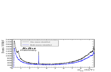
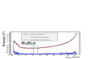
Figure 1: Distribution of the dimuon invariant mass $m_{\mu^{+}\mu^{-}}$ in the $\mathchar 28935\relax{(3S)}$ data is shown on the left. Statistical and systematic uncertainty on the product of branching fractions $\mathcal{B}(\mathchar 28935\relax{(3S)}\rightarrow\gamma{A^{0}})\times\mathcal{B}({A^{0}}\rightarrow\mu^{+}\mu^{-})$ are shown on the right as a function of $m_{A^{0}}$, extracted from the fits to the $\mathchar 28935\relax{(3S)}$ data. Statistical errors are shown as red dot-dashed line, systematic uncertainties are shown as blue dotted line, and the total uncertainty, computed as a quadrature sum of statistical and systematic errors, is the solid black line. The shaded areas show the regions around the ${J\mskip-3.0mu/\mskip-2.0mu\psi\mskip 2.0mu}$ and $\psi(2S)$ resonances excluded from the search.

6 RESULTS for $A^{0}\rightarrow\mu^{+}\mu^{-}$

For a small number of fits in the scan over the $\mathchar 28935\relax{(3S)}$ dataset, we observe local likelihood ratio values $\mathcal{S}$ of about $3\sigma$. The most significant peak is at $m_{A^{0}}=4.940\pm 0.003$ $\mathrm{\,Ge\kern-1.00006ptV}$ (likelihood ratio value $\mathcal{S}=3.0$, including systematics; ${\cal B}=(1.9\pm 0.7\pm 0.1)\times 10^{-6}$). The second most-significant peak is at $m_{A^{0}}=0.426\pm 0.001$ $\mathrm{\,Ge\kern-1.00006ptV}$ (likelihood ratio value $\mathcal{S}=2.9$, including systematics; ${\cal B}=(3.1\pm 1.1\pm 0.3)\times 10^{-6}$). The peak at $m_{A^{0}}=4.940$ $\mathrm{\,Ge\kern-1.00006ptV}$ is theoretically disfavored (since it is significantly above the $\tau$ threshold), while the peak at $m_{A^{0}}=0.426$ $\mathrm{\,Ge\kern-1.00006ptV}$ is in the range predicted by the axion model [11]. However, since our scans have $\mathcal{O}(2000)$ $m_{A^{0}}$ points, we should expect several statistical fluctuations at the level of $\mathcal{S}\approx 3$, even for a null signal hypothesis. At least 80% of our pseudo-experiments contain a fluctuation with $\mathcal{S}=3\sigma$ or more. Taking this into account, we conclude that neither of the above-mentioned peaks are significant.

Since we do not observe a significant excess of events above the background in the range $0.212<m_{A^{0}}\leq 9.3$ GeV, we set upper limits on the branching fraction $\mathcal{B}(\mathchar 28935\relax{(3S)}\rightarrow\gamma{A^{0}})\times\mathcal{B}({A^{0}}\rightarrow\mu^{+}\mu^{-})$. We add statistical and systematic uncertainties (which include the additive errors on the signal yield and multiplicative uncertainties on the signal efficiency and the number of recorded $\mathchar 28935\relax{(3S)}$ decays) in quadrature. The 90% C.L. Bayesian upper limits, computed with a uniform prior and assuming a Gaussian likelihood function, are shown in Fig. 2 (right), as a function of mass $m_{A^{0}}$. The limits fluctuate depending on the central value of the signal yield returned by a particular fit, and range from $0.25\times 10^{-6}$ to $5.2\times 10^{-6}$.

We do not observe any significant signal at the HyperCP mass, $m_{A^{0}}=0.214$ $\mathrm{\,Ge\kern-1.00006ptV}$. We find ${\cal B}(\mathchar 28935\relax{(3S)}\rightarrow\gamma A^{0}(214))=(0.12^{+0.43}_{-0.41}\pm 0.17)\times 10^{-6}$, and set an upper limit ${\cal B}(\mathchar 28935\relax{(3S)}\rightarrow\gamma A^{0}(214))<0.8\times 10^{-6}$ at 90% C.L.

From a fit to the $\eta_{b}$ region, we find ${\cal B}(\mathchar 28935\relax{(3S)}\rightarrow\gamma\eta_{b})\times{\cal B}(\eta_{b}\rightarrow\mu^{+}\mu^{-})=(0.2\pm 3.0\pm 0.9)\times 10^{-6}$, consistent with zero. Taking into account the BABAR measurement of ${\cal B}(\mathchar 28935\relax{(3S)}\rightarrow\gamma\eta_{b})=(4.8\pm 0.5\pm 1.2)\times 10^{-4}$, we can derive ${\cal B}(\eta_{b}\rightarrow\mu^{+}\mu^{-})=(0.0\pm 0.6\pm 0.2)\%$, or an upper limit ${\cal B}(\eta_{b}\rightarrow\mu^{+}\mu^{-})<0.8\%$ at 90% C.L. This is consistent with expectations from the quark model. All results above are preliminary.

The limits we set [15] are more stringent than those recently reported by the CLEO collaboration [16]. Our limits rule out much of the parameter space allowed by the light Higgs [10] and axion [11] models.

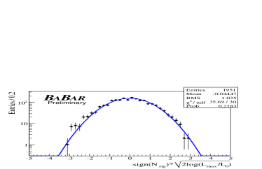
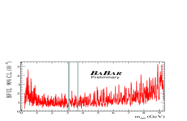
Figure 2: Distribution of the likelihood ratio variable $\mathcal{S}$ with additive systematic uncertainties included for the fits to the $\mathchar 28935\relax{(3S)}$ dataset, overlayed with a blue curve showing the Gaussian fit with fixed $\mu=0$ and $\sigma=1$, is shown on the left. Upper limits on the product of branching fractions ${\cal B}(\mathchar 28935\relax{(3S)}\rightarrow\gamma A^{0})\times{\cal B}(A^{0}\rightarrow\mu^{+}\mu^{-})$ as a function of $m_{A^{0}}$ from the fits to $\mathchar 28935\relax{(3S)}$ data are shown on the right. The shaded areas show the regions around the ${J\mskip-3.0mu/\mskip-2.0mu\psi\mskip 2.0mu}$ and $\psi(2S)$ resonances excluded from the search.

7 CONCLUSIONS

We find no evidence for light Higgs boson in a sample of $122\times 10^{6}$ $\mathchar 28935\relax(3S)$ decays collected by the BABAR collaboration at the PEP-II B-factory, and set 90% C.L. upper limits on the product of the branching fractions $\mathcal{B}(\mathchar 28935\relax(3S)\rightarrow\gamma A^{0})\times\mathcal{B}(A^{0}\rightarrow\mathrm{invisible})$ at $(0.7-31)\times 10^{-6}$ in the mass range $m_{A^{0}}\leq 7.8$ GeV [14] and on the product $\mathcal{B}(\mathchar 28935\relax(3S)\rightarrow\gamma A^{0})\times\mathcal{B}(A^{0}\rightarrow\mu^{+}\mu^{-})$ at $(0.25-5.2)\times 10^{-6}$ in the mass range $0.212\leq m_{A^{0}}\leq 9.3$ GeV [15]. We also set a limit on the dimuon branching fraction of the recently discovered $\eta_{b}$ meson ${\cal B}(\eta_{b}\rightarrow\mu^{+}\mu^{-})<0.8\%$ at 90% C.L. [15]. The results are preliminary.

References

- [1] P.W. Higgs Phys. Rev. Lett. 13, 508 (1964).
- [2] S. Weinberg, Phys. Rev. Lett. 19, 1264 (1967); A. Salam, p. 367 of Elementary Particle Theory, ed. N. Svartholm (Almquist and Wiksells, Stockholm, 1969); S.L. Glashow, J. Iliopoulos, and L. Maiani, Phys. Rev. D 2, 1285 (1970).
- [3] LEP Working Group for Higgs boson searches, R. Barate et al., Phys. Lett. B565, 61 (2003).
- [4] M. Herndon, rapporteur talk at ICHEP ’08, arXiv:0810.3705 [hep-ex] (2008).
- [5] LEP-SLC Electroweak Working Group, Phys. Rept. 427, 257 (2006).
- [6] J. Wess and B. Zumino, Nucl. Phys. B70, 39 (1974).
- [7] R. Dermisek and J.F. Gunion, Phys. Rev. Lett. 95, 041801 (2005).
- [8] R. Dermisek and J.F. Gunion, Phys. Rev. D 73, 111701 (2006).
- [9] F. Wilczek, Phys. Rev. Lett. 39, 1304 (1977).
- [10] R. Dermisek, J.F. Gunion, and B. McElrath, Phys. Rev. D 76, 051105 (2007).
- [11] Y. Nomura and J. Thaler, preprint arXiv:0810.5397 [hep-ph] (2008).
- [12] H. Park et al., HyperCP Collaboration, Phys. Rev. Lett. 94, 021801 (2005).
- [13] X. G. He, J. Tandean and G. Valencia, Phys. Rev. Lett. 98, 081802 (2007).
- [14] B. Aubert et al., BABAR Collaboration, arXiv:0808.0017 [hep-ex].
- [15] B. Aubert et al., BABAR Collaboration, arXiv:0902.2176 [hep-ex].
- [16] W. Love, et al., CLEO Collaboration, Phys. Rev. Lett. 101, 151802 (2008).
- [17] E. Fullana and M.A. Sanchis-Lozano, Phys. Lett. B 653, 67 (2007).
- [18] B. Aubert et al., BABAR Collaboration, Phys. Rev. Lett. 101, 071801 (2008).
- [19] B. Aubert et al., BABAR Collaboration, Nucl. Instrum. Methods Phys. Res., Sect. A 479, 1 (2002).
- [20] S. Agostinelli et al., GEANT4 Collaboration, Nucl. Instrum. Methods Phys. Res., Sect. A 506, 250 (2003).
- [21] M. J. Oreglia, Ph.D Thesis, report SLAC-236 (1980), Appendix D; J. E. Gaiser, Ph.D Thesis, report SLAC-255 (1982), Appendix F; T. Skwarnicki, Ph.D Thesis, report DESY F31-86-02(1986), Appendix E.