Nonlinear response of a thin metamaterial film containing Josephson junctions

Abstract

An interaction of electromagnetic field with metamaterial thin film containing split-ring resonators with Josephson junctions is considered. It is shown that dynamical self-inductance in a split rings results in reduction of magnetic flux through a ring and this reduction is proportional to a time derivative of split ring magnetization. Evolution of thin film magnetization taking into account dynamical self-inductance is studied. New mechanism for excitation of waves in one dimensional array of split-ring resonators with Josephson junctions is proposed. Nonlinear magnetic susceptibility of such thin films is obtained in the weak amplitude approximation.

1 Introduction

During the last decade metamaterials have become the focus of intensive research [1, 2, 3]. The nonlinear electrodynamics of metamaterials is of special interest due to the presence of new nonlinear phenomena which are specific to metamaterials [4, 5, 6] and due to the fact that, in several cases, nonlinearity is a characteristic feature of nanoscale systems [7, 8]. The nonlinear response of metamaterials can also be the result of deliberate design. For example, nonlinear dielectrics or diodes can be inserted into split rings [9, 10]. Josephson junctions (JJ) are known to be strongly nonlinear [11] with low losses and therefore they are a natural way to introduce nonlinearity in metamaterials. Electromagnetic field interaction with metamaterials containing split-rings with Josephson junctions inserted into the gap was recently considered in several papers. For example, localized oscillations in chains and two dimensional arrays of such split-rings were considered in [12, 13, 14]. The existence of metastable states in a medium of this type and transitions between these states was discussed in [15].

Currently metamaterials primarily exist in the form of thin films. Thus, it is a clear choice to study the interaction of an electromagnetic wave with thin films containing strongly nonlinear structural units. Split-rings containing Josephson junctions are natural building blocks for such thin films. This subject is considered in the first section of this paper. In particular, we investigated the effect of dynamical self-inductance in split rings which results in reduction of magnetic flux through a ring. This reduction is proportional to the time derivative of split ring magnetization. This effect manifests itself as non Fresnellian reflection from a film and represents an additional mechanism increasing rate of oscillation relaxation in ring-resonators. We show that this additional damping leads to dramatic change in the evolution dynamics of film magnetization.

The interaction of a chain of split-rings containing JJ with an electromagnetic field is considered in the second section. We expressed the individual current of a particular ring in terms of magnetic fluxes through all other rings in a chain. In continuous limit, taking into account near neighbor interactions to leading order, we obtained sine-Gordon type of equation describing ”continuous” chain dynamics. The effect of dynamical self inductance is presented in this model as an additional damping term. External force in this equation contains the second spatial derivatives of the incident field and therefore suggests a new mechanism for the excitation of longitudinal oscillations by a normally incident field (without tangential component along the chain).

In the third section, we obtained the nonlinear magnetic susceptibility of a thin film containing split-rings with JJ in the limit of weak amplitudes. This susceptibility describes third harmonic generation and self modulation due to high frequency Kerr effect.

2 Electromagnetic wave interaction with thin films containing Josephson junctions

Electromagnetic field interaction with thin films ($\Delta x\ll\lambda$) is a well studied subject in the literature [16, 17, 18, 19, 20, 21, 22, 23]. Most of these works consider thin films being polarized under an external field. In this paper we study magnetoactive thin films. This requires the derivation of new modeling equations which we present in the following subsection.

2.1 Transmission and reflection of electromagnetic wave on magnetoactive thin films: basic equations

We consider a plane electromagnetic wave normally incident from $-\infty$ along the $x$ axis on a magnetoactive thin film. The corresponding Maxwell equations have following form:

$$\frac{\partial H_{y}}{\partial x}=\frac{1}{c}\frac{\partial D_{z}}{\partial t},~{}~{}\frac{\partial E_{z}}{\partial x}=\frac{1}{c}\frac{\partial B_{y}}{\partial t}.$$ (1)

We take into account only magnetic response. Total magnetic inductance reads as

$$B_{y}(x,t)=B^{host}(x,t)+4\pi M(t)\delta(x).$$

Here magnetization of the thin film $\approx lM^{(s)}$ can be represented as a product of surface magnetization $M^{(s)}$ and the width of the film $l$. $B^{host}(x,t)$ is the magnetic inductance of the host material. Integrating the equations (1) over $x$ from $-\delta x$ to $+\delta x$ and taking the limit $\delta x\rightarrow 0$ leads to the boundary conditions at the point $x=0$:

$$H_{y}(0-) = H_{y}(0+),$$ (2)

$$E_{z}(0-)-E_{z}(0+) = -\frac{4\pi l}{c}\frac{\partial M^{(s)}}{\partial t}.$$ (3)

In a homogeneous medium for $x<0$ and at $x>0$ the system of equations (1) can be reduced to the wave equation

$$\frac{\partial^{2}H}{\partial x^{2}}=\frac{\varepsilon}{c}\frac{\partial^{2}H}{\partial t^{2}}$$ (4)

where $\varepsilon=\varepsilon_{1}$ for $x<0$ and $\varepsilon=\varepsilon_{2}$ for $x>0$. Introducing variables $q_{j}=k_{0}\sqrt{\varepsilon_{j}},\,j=1,2$ and $k_{0}=\omega/c$ we can represent the solution of (4) in terms of Fourier components as follows:

$$\tilde{H}(x,\omega)=\left\{\begin{array}[]{lr}Ae^{iq_{1}x}+Be^{-iq_{1}x},&x<0,\\ Ce^{iq_{2}x},&x>0,\end{array}\right.$$ (5)

For the electric field we have

$$\tilde{E}_{z}(x,\omega)=\left\{\begin{array}[]{lr}-q_{1}(\varepsilon_{1}k_{0})^{-1}\left(Ae^{iq_{1}x}-Be^{-iq_{1}x}\right),&x<0,\\ -q_{2}(\varepsilon_{2}k_{0})^{-1}Ce^{iq_{2}x},&x>0,\end{array}\right.$$ (6)

Taking into account boundary conditions (2) and (3) we obtain relations

$$A+B = C,$$

$$\frac{iq_{1}}{\varepsilon_{1}}(A-B) = \frac{iq_{2}}{\varepsilon_{2}}C+4\pi k_{0}^{2}l\tilde{M}^{(s)},$$

which define the amplitudes $B,C$ via the amplitude of the incident wave $A=\tilde{H}^{in}$:

$$\tilde{H}^{(tr)}=C=\frac{2\varepsilon_{2}q_{1}}{\varepsilon_{2}q_{1}+\varepsilon_{1}q_{2}}\tilde{H}^{(in)}+\frac{4i\pi k_{0}^{2}l\varepsilon_{1}\varepsilon_{2}}{\varepsilon_{2}q_{1}+\varepsilon_{1}q_{2}}\tilde{M}^{(s)},$$ (7)

$$\tilde{H}^{(ref)}=B=\frac{\varepsilon_{2}q_{1}-\varepsilon_{1}q_{2}}{\varepsilon_{2}q_{1}+\varepsilon_{1}q_{2}}\tilde{H}^{(in)}+\frac{4i\pi k_{0}^{2}l\varepsilon_{1}\varepsilon_{2}}{\varepsilon_{2}q_{1}+\varepsilon_{1}q_{2}}\tilde{M}^{(s)}.$$ (8)

In the simplest case when $\varepsilon_{1}=\varepsilon_{2}=\varepsilon$ and dispersion of the host material is negligible ($\varepsilon=const$), expression (7) can be rewritten as

$$\tilde{H}^{(tr)}=\tilde{H}^{(in)}+\frac{2i\pi l\omega\sqrt{\varepsilon}}{c}\tilde{M}^{(s)}.$$

In temporal and spatial variables it reads as

$$H^{tr}(t)=H^{(in)}(t)-\frac{2\pi l\sqrt{\varepsilon}}{c}\frac{\partial M^{(s)}}{\partial t}.$$ (9)

The expression for magnetic field inside the film $H(t)=H^{(tr)}$ follows from the continuity condition for the tangential components of the magnetic field (2). For further analysis we need to determine properties of the magnetization $M^{(s)}$ for the film containing Josephson junctions.

2.2 Magnetic response of split-rings with Josephson junctions

We consider a thin film composed of split rings with Josephson junctions in their gaps (see Fig. 1). Orientation of the magnetic field is orthogonal to the split ring’s plane.

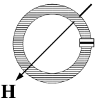
Figure 1: Schematic of a split ring with Josepson junction in the gap. Magnetic field H is orthogonal to the plane of a split ring.

Fig. 2 shows an equivalent electric circuit of a split ring with Josephson junction [25]. Here $\mathcal{E}$ stands for electromotive force, $L$ is inductance of a split ring, $C$ and $R$ are capacitance and resistance of a Josephson junction. The electromotive force connected with the magnetic flux $\Phi$ is in accordance with Faraday’s law:

$$\mathcal{E}=-\frac{1}{c}\frac{d\Phi}{dt}.$$ (10)

Figure 2: Equivalent electric circuit of a ring with Josephson junction. Here $E$ stands for electromotive force, $L$ is inductance of a split ring, $C$ and $R$ are capacitance and resistance of a Josephson junction.

Self-induced electromotive force inductance $U_{L}$ can be expressed via current $J$ through inductance $L$:

$$U_{L}=\frac{L}{c^{2}}\frac{dJ}{dt}.$$ (11)

Josephson voltage $U_{C}$ and current $J_{j}$ are defined by following expressions [24, 26]:

$$U_{C}=\frac{\hbar}{2e}\frac{d\phi}{dt},~{}~{}~{}J_{j}=J_{0}\sin\phi$$ (12)

In accordance to Kirchhoff laws the sum of the electrical potential differences in a circuit is equal to an electromotive force

$$\mathcal{E}=U_{L}+U_{C},$$ (13)

and the sum of currents flowing towards that point is equal to the sum of currents flowing away from that point, i.e.

$$J_{j}+J_{R}+J_{C}=J.$$ (14)

The equation (13) gives

$$\frac{1}{c}\Phi+\frac{L}{c^{2}}J+\frac{\hbar}{2e}\phi=0$$ (15)

As follows from (15) the current $J$ can be expressed in the following form

$$J=-\frac{c}{L}\left(\Phi+\frac{\hbar c}{2e}\phi\right)$$ (16)

Let us consider the second Kirchhoff equation (14). Variables in the equation (14) are defined as follows

$$J_{C} = C\frac{dU_{C}}{dt}=C\frac{\hbar}{2e}\frac{d^{2}\phi}{dt^{2}},$$

$$J_{R} = \frac{U_{C}}{R}=\frac{\hbar}{2eR}\frac{d\phi}{dt}$$

The second Kirchhoff equation (14) transforms to

$$\frac{d^{2}\phi}{dt^{2}}+\frac{1}{RC}\frac{d\phi}{dt}+\frac{c^{2}}{LC}\phi+\frac{2eJ_{0}}{\hbar C}\sin\phi=-\frac{2ec}{\hbar LC}\Phi$$ (17)

Magnetic flux is determined by the external magnetic field $H$ and by a cross section of a split ring with radius $a$:

$$\Phi=\int_{S}Hds\approx\pi a^{2}H.$$ (18)

The modulus of magnetization vector can be defined as

$$M=\rho\frac{\pi a^{2}}{c}J,$$ (19)

where $\rho$ is the density of currents (or contours). Thus magnetic response is governed by the following system

$$\frac{d^{2}\phi}{dt^{2}}+\frac{1}{RC}\frac{d\phi}{dt}+\frac{c^{2}}{LC}\phi+\frac{2eJ_{0}}{\hbar C}\sin\phi=-\frac{2ec\pi a^{2}}{\hbar LC}H$$ (20)

$$M=-\frac{\pi a^{2}\rho}{L}\left(\Phi+\frac{\hbar c}{2e}\phi\right)$$ (21)

Flux and magnetic field in (24) and (21) can be expressed via the external magnetic field using equation (9). Thus equations  (24) and (21) can be rewritten in the following form

$$\frac{\partial^{2}\phi}{\partial t^{2}} + \Gamma\frac{\partial\phi}{\partial t}+\omega_{T}^{2}\phi+\vartheta\sin\phi=$$ (22)

$$= -\frac{2ec(\pi a^{2})}{CL\hbar}\left[H^{(in)}-\frac{4\pi\sqrt{\varepsilon}l}{c}\frac{\partial M^{(s)}}{\partial t}\right],$$

$$M^{(s)} = -\frac{\pi a^{2}\rho}{L}\left(\frac{\hbar c}{2e}\phi+\pi a^{2}H^{(in)}\right).$$ (23)

Here $\omega_{T}$ is Thomson frequency ($\omega_{T}^{2}=c^{2}/CL$), coefficient $\Gamma=1/CR$ describes dissipation, and $\vartheta=(2eJ_{0})/(C\hbar)$ determines strength of nonlinearity. The coefficient $\hbar/2e$ can be represented via the quantum of magnetic flux $\Phi_{0}=\pi\hbar c/e$. Let us introduce dimensionless variables using following scaling:

$$H^{in}(t)=\frac{\hbar c}{2e\pi a^{2}}h(t/\tau_{0}),~{}~{}\tau_{0}=\omega_{T}^{-1},$$

$$M(t)=\frac{\hbar c\pi a^{2}\rho}{2eL}m(t/\tau_{0}).$$

The system of equations (22) and (23) in new variables reads

$$\frac{\partial^{2}\phi}{\partial\tau^{2}}+\gamma\frac{\partial\phi}{\partial\tau}+\phi+\kappa\sin\phi=-\left(h-\delta\psi\right),$$

$$\psi=-\left(\frac{\partial\phi}{\partial\tau}+\frac{\partial h}{\partial\tau}\right),$$ (24)

here $\tau=\omega_{T}t$, $\gamma=\Gamma/\omega_{T}$, $\kappa=\vartheta/\omega_{T}^{2}$ and

$$\delta=l\left[\frac{4\pi\sqrt{\epsilon}\rho(\pi a^{2})^{2}\omega_{T}}{cL}\right]=l\left[\frac{4\pi\sqrt{\epsilon}\rho(\pi a^{2})^{2}}{L\sqrt{LC}}\right].$$

This model describes the magnetic response of a thin film with a diluted concentration of split rings containing Josephson junctions. Interaction of split rings in this case occurs only via the external electromagnetic field. Effects of near neighbor interaction between split rings were considered in the literature and can be found in [12, 13, 28, 29, 14]. Work presented in [12, 28, 29] considers interacting split rings without Josephson junctions. Dense arrangement of split rings with Josephson junctions, which requires consideration of near neighbor interactions is presented in [13, 14]. In these papers the external force acting on an array of split rings was determined only by external magnetic field. Based on this work we derive a generalization of the model presented in [13, 14]. Our equations take into account the influence of an additional magnetic field due to induced magnetization of a split rings. This additional effect is accounted for by the second term in the equation (9). This effect results in an increase of the energy dissipation rate due to field radiation from the film. An additional dissipation changes the magnetization relaxation process to the equilibrium states. Additionally, the effect of induced magnetization results in a strong dependance of relaxation process on the frequency of external field.

2.3 Impact of dynamical magnetic self inductance

Evolution of a magnetic field described by the equations (24) can be illustrated in terms of the dynamics of a Newtonian particle in the potential

$$U(\phi)=\frac{1}{2}\phi^{2}-\kappa\cos\phi.$$

This potential can have different numbers of minima (stable stationary points). The number of such minima is determined by the value of $\kappa$. Fig. 3 illustrates a potential with one minimum (solid line), where $\kappa=1$, and with three minima (dashed line), where $\kappa=8$. Two maxima corresponding to the last case describe unstable states. First we consider potential with one minimum.

Figure 3: Graph illustrates the dependance of potential $U(\phi)=\phi^{2}/2-\kappa\cos{\phi}$ on $\phi$. The potential can have several minima. Solid line illustrates one minimum potential ($\kappa=1$), dashed line illustrates three minimum potential ($\kappa=8$).

From Equations (24) it follows that taking into account the effect of self induced magnetization results in the increase of damping factor $\gamma\rightarrow\gamma+\delta$. This effect is illustrated in Fig. 4. The left subfigure in Fig. 4 shows the relaxation of magnetization without taking into account self induced magnetization, and the right subfigure shows relaxation in the presence of self induced magnetization. The relaxation process, which is shown in the right subfigure is faster than relaxation in the left figure. Magnetization in this case is excited by an external magnetic field of a gaussian shape $h(t)=a\exp\left[-(t/t_{0})\right]$, $a=4.5$ and $t_{0}=0.5$. Parameters of the equations (24) for this example have been chosen as follows: $\kappa=1$, $\gamma=0.05$, $\delta=0.02$

Figure 4: Magnetization relaxation in the case when self induced magnetization of a split ring is not taken into account - left figure and is taken into account -right figure. Magnetization is excited by by incident spike of the gaussian shape $h(t)=a\exp\left[-(t/t_{0})\right]$, $a=4.5$ and $t_{0}=0.5$. Evolution takes place in a single minimum potential $U(\phi)=\phi^{2}/2-\ \cos{\phi}$ ($\kappa=1$ - solid line on Fig. 3).

Second, we consider the evolution of magnetization in the case of a three minimum potential. The difference in the evolution of magnetization between the two cases with and without self induced magnetization is more dramatic in a three minimum potential. There are four oscillatory regimes corresponding to oscillations around the central minimum, around the two side minima and when oscillations are taking place above two local maxima of the potential (see Fig. 3). These types of oscillations have different frequencies and, in the last case, the period of oscillations is largest and the amplitude is limited from below. Fig. 5 shows the dynamics of magnetization with and without self induced magnetization for the same values of parameters and external magnetic field.

Figure 5: Magnetization relaxation in the case when self induced magnetization of a split ring is not taken into account - left figure and is taken into account -right figure. Magnetization is excited by by incident spike of the gaussian shape $h(t)=a\exp\left[-(t/t_{0})\right]$, $a=12.1$ and $t_{0}=0.5$. Evolution takes place in a two minima potential $U(\phi)=\phi^{2}/2-\kappa\cos{\phi}$ ($\kappa=8$ - dashed line on Fig. 3).

The initially excited oscillations corresponding to the trajectories of Newtonian particles above local minima of the potential are decaying and eventually switching to faster and lower amplitude oscillations around one of the minima. The moment of switching and asymptotic stable state is highly sensitive to the presence of self induced magnetization. In this particular case, which is illustrated in Fig. 5, switching to oscillations around the central minimum occurs after seven cycles of large amplitude oscillations - left subfigure. The presence of an additional decay in relaxation of magnetization due to self induced magnetization, which results in excessive radiation, results in the switching to oscillations around right minima only after three and a half oscillatory cycles - right subfigure. In both cases oscillations are excited by an external spike of the magnetic field $h(t)=a\exp\left[-(t/t_{0})\right]$, $a=12.1$ and $t_{0}=0.5$, where $\kappa=8$.

2.4 Multistability of magnetization

The mirrorless optical bistability has been predicted in a bulk [18] and in the thin film [19] of dipole-dipole interacting two-level atoms. We can expect this effect in the case under consideration too. In the case of stationary fields, system (24) reads as

$$(m+h)+\kappa\sin(m+h)=h,~{}~{}~{}h=const,$$ (25)

This is an implicit equation for $\phi$ as function of $h$. The general solution of (25) can have several roots. For a three minimum potential, the solution is illustrated in Fig. 6.

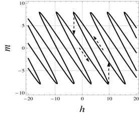
Figure 6: Graph illustrates multistability of magnetization $m$ versus value of stationary magnetic field $h$. Parameters of three minima potential are $\kappa=8$ - dashed line on Fig. 3).

The presence of three stable and two unstable stationary solutions leads to the multivalued nature of the function $\phi(h)$, which results in multistability of magnetization. This function consists of stable and unstable branches, which lead to hierarchical set of hysteresis loops. The simplest first order hysteresis loop is shown in Fig. 6.

3 Near neighbor interaction interaction between split rings

Following the work in [12] let us take into account the magnetic dipole-dipole interaction between neighboring SRRs characterized by cross-inductance $L_{cross}$. Note that cross-inductance decays as the cube of the distance. Let us restrict ourself to only nearest neighbor SRR interactions.

The voltage on the $n$th junction is expressed via phase $\phi_{n}$ as

$$U_{n,c}=\frac{\hbar}{2e}\frac{\partial\phi_{n}}{\partial t}$$ (26)

The voltage on the junction is equal to $U_{n,C}$ and is also equal to the voltage $U_{n,R}$. Thus the normal (i.e., non superfluid) current thought the junction is $U_{n,c}/R$.

According to Kirchhoff law, voltage on the ring is equal to the sum of acting electromotive forces. Therefore, the first Kirchhoff’s equation has following form:

$$U_{n,c}=-\frac{L}{c^{2}}\frac{\partial I_{n}}{\partial t}-\frac{L_{cross}}{c^{2}}\left(\frac{\partial I_{n-1}}{\partial t}+\frac{\partial I_{n+1}}{\partial t}\right)-\mathcal{E}_{n}$$ (27)

Here $\mathcal{E}_{n}=-c^{-1}d\Phi_{n}/dt$ is electromotive force induction generated by high frequency magnetic flux acting on $n$th ring, $I_{n\pm 1}$ is the current in the $(n\pm 1)$th ring.

The second Kirchhoff equation corresponds to charge conservation:

$$I_{n}=J_{n}+C_{n}\frac{\partial U_{n,c}}{\partial t}+\frac{U_{n,c}}{R}$$ (28)

Combining equation (26) with (27) we obtain

$$I_{n}+\eta\left(I_{n-1}+I_{n+1}\right)=-\frac{c}{L}\left(\Phi_{n}+\frac{c\hbar}{2e}\phi_{n}\right),$$ (29)

where $\eta=L_{cross}/L$. This equation must be complemented with equations defining currents at each split-ring:

$$I_{n}=J_{0n}\sin\phi_{n}+\frac{C\hbar}{2e}\frac{\partial^{2}\phi_{n}}{\partial t^{2}}+\frac{\hbar}{2er}\frac{\partial\phi_{n}}{\partial t}.$$ (30)

Expression (29) represents a linear recurrency relation. In the limit $N\rightarrow\infty$, we can employ the generating function method.

3.1 Calculation of individual currents in a split rings

Let us introduce notation

$$F_{n}=-\frac{c}{L}\left(\Phi_{n}+\frac{c\hbar}{2e}\phi_{n}\right).$$

and rewrite equation (29) as

$$I_{n}+\eta\left(I_{n-1}+I_{n+1}\right)=F_{n},$$ (31)

Introducing the generating function

$$P(y)=\sum\limits_{n=-\infty}^{+\infty}I_{n}e^{iny},$$

defining the function $F(y)$

$$F(y)=\sum\limits_{n=-\infty}^{+\infty}F_{n}e^{iny}$$ (32)

and using equation (31) we can find relation between $P(y)$ and $F(y)$

$$P(y)=\frac{F(y)}{1+2\eta\cos y}.$$ (33)

This expression can be represented as a power series

$$P(y)=\sum_{m=0}^{\infty}(-2\eta)^{m}\cos^{m}(y)F(y).$$

Function $\cos^{m}(y)$ can be expressed as

$$\cos^{m}(y) = 2^{-m}e^{imy}\left(1+e^{-2iy}\right)^{m}=$$

$$= 2^{-m}e^{imy}\sum_{p=0}^{m}\binom{m}{p}e^{-2ipy},$$

then the generating function has the form:

$$P(y)=\sum_{m=0}^{\infty}(-2\eta)^{m}\sum_{p=0}^{m}\binom{m}{p}e^{-iy(m-2p)}F(y).$$

The current in the $n$-th ring is determined by the formula

$$I_{n}=(2\pi)^{-1}\int_{-\infty}^{+\infty}P(y)e^{iny}dy.$$

Using the expression for $F(y)$ (32) we can find that

$$I_{n}(t)=\sum_{m=0}^{\infty}(-\eta)^{m}\sum_{p=0}^{m}\binom{m}{p}F_{n+m-2p}(t).$$ (34)

The expression for $I_{n}$ can be simplified taking into account smallness of the parameter $\eta\ll 1$. Up to the second order of $\eta$, the expression for $I_{n}(t)$ has the form

$$I_{n}(t) \approx F_{n}(t)-\eta\left(F_{n+1}(t)+F_{n-1}(t)\right)+$$ (35)

$$+ \eta^{2}\left(F_{n+2}(t)+2F_{n}(t)+F_{n-2}(t)\right).$$

3.2 Continuum chain approximation

In the continuum approximation we can introduce a new variable $y=nl_{r}$, where $l_{r}$ is the distance between neighboring rings, and represent $F_{n\pm 1}(t)$ as

$$F_{n\pm 1}(t)\approx F(y)(t)\pm l_{r}\frac{\partial F}{\partial y}+\frac{l_{r}^{2}}{2}\frac{\partial^{2}F}{\partial y^{2}}.$$

Limiting ourself to the first order expansion with respect to $\eta$ we obtain from (35)

$$I(y,t) \approx (1-2\eta)F(y,t)-\eta l_{r}^{2}\frac{\partial^{2}}{\partial y^{2}}F(y,t)$$ (36)

$$\approx F(y,t)-\eta l_{r}^{2}\frac{\partial^{2}}{\partial y^{2}}F(y,t).$$

In our model $F(y,t)$ was defined as

$$F(y,t)=-\frac{c}{L}\left(\Phi(y,t)+\frac{c\hbar}{2e}\phi(y,t)\right)$$

Since the magnetic flux through ring is greater than the flux through the junction (gap), we can use the approximate expression $\Phi(y,t)\approx(\pi a^{2})H(y,t)$. Substitution of this expression in (30) leads to

$$J_{0n}\sin\phi_{n} + \frac{C\hbar}{2e}\frac{\partial^{2}\phi_{n}}{\partial t^{2}}+\frac{\hbar}{2eR}\frac{\partial\phi_{n}}{\partial t}=$$ (37)

$$= -\frac{c}{L}\left(\Phi(y,t)+\frac{c\hbar}{2e}\phi(y,t)\right)+$$

$$+ \frac{\eta l_{r}^{2}c}{L}\left(\frac{\partial^{2}\Phi}{\partial y^{2}}+\frac{c\hbar}{2e}\frac{\partial^{2}\phi}{\partial y^{2}}\right).$$

Using dimensionless variables defined above, the resulting system of equations can be written as

$$\frac{\partial^{2}\phi}{\partial\tau^{2}} - \frac{\partial^{2}\phi}{\partial\xi^{2}}+\gamma\frac{\partial\phi}{\partial\tau}+\phi+\kappa\sin\phi=$$ (38)

$$= -\left(h-\delta\psi\right)+\frac{\partial^{2}}{\partial\xi^{2}}\left(h-\delta\psi\right),$$

$$\psi = -\left(\frac{\partial\phi}{\partial\tau}+\frac{\partial h}{\partial\tau}\right).$$ (39)

Here we introduce dimensionless spatial variable $\xi=y/(l_{r}\sqrt{\eta})$.

In case of plane electromagnetic wave propagating along $x$, dependence of $h$ on $y$ vanishes. Spatial derivatives in the equation (39) disappear and equation describes homogeneous dynamics of the chain as function of time. Temporal-spatial chain dynamics takes place when the chain is excited by an electromagnetic beam with spatial distribution of intensity across the beam. In the general case, excitation of surface waves requires matching of the surface wave vector with tangential component of the vector of the incident wave. Equation (38) demonstrates that sharp spatial gradients across the beam act as an external force for oscillations along the chain.

4 Small-amplitude approximation in SRRs

In the linear approximation equation (22) reads

$$\frac{\partial^{2}\phi}{\partial t^{2}}+\frac{1}{Cr}\frac{\partial\phi}{\partial t}+\Omega^{2}\phi=-\frac{2ec}{CL\hbar}\Phi(t)$$ (40)

where $\Omega$ is renormalized Thompson frequency $\Omega^{2}=(LC/c^{2})^{-1}+(2eJ_{0}/C\hbar)$. The Fourier components of current are represented as

$$I(\omega)=\frac{\pi a^{2}c}{L}\left(\frac{\omega_{T}^{2}}{\Omega^{2}-\omega^{2}-i\Gamma\omega}-1\right)H(\omega).$$

Fourier components of magnetic induction $B=H+4\pi M$ are expressed through magnetic permittivity $B=\mu(\omega)H$, which leads to

$$\mu(\omega)=1+4\pi n_{m}\frac{(\pi a^{2})^{2}}{L}\left(\frac{\omega_{T}^{2}}{\Omega^{2}-\omega^{2}-i\Gamma\omega}-1\right)$$

Since equation (22) is nonlinear, the magnetic response is described by a nonlinear coupling between field $H$ and magnetization $M$. The total magnetization can be represented as sum of a linear part $M_{lin}$ and nonlinear part $M_{nl}$. Taking into account the definition of magnetization (23) we obtain following expressions

$$M_{lin}=-n_{m}\frac{\pi a^{2}}{L}\left(\pi a^{2}H+\frac{\hbar c}{2e}\phi^{(0)}\right),$$

$$M_{nl}=-n_{m}\frac{\pi a^{2}}{L}\frac{\hbar c}{2e}\phi^{(1)},$$

where $\phi^{(0)}$ is solution of the linear equation, and $\phi^{(1)}$ is correction to solution of the linear equation (40).

Expansion of sine-function up to cubic term $\phi^{3}$), transforms (22) into the Duffing equation:

$$\frac{\partial^{2}\phi}{\partial t^{2}}+\Gamma\frac{\partial\phi}{\partial t}+\Omega^{2}\phi+\vartheta\phi^{3}=-\frac{2ec}{CL\hbar}\Phi(t)$$ (41)

where $\vartheta=2eJ_{0}/6c\hbar$ is parameter characterizing nonlinear response of Duffing oscillator. Let us consider only the first correction term for solution of (22). Substituting $\phi=\phi^{(0)}+\phi^{(1)}$ into (22) and collecting terms of same order we obtain:

$$\frac{\partial^{2}\phi^{(0)}}{\partial t^{2}}+\Gamma\frac{\partial\phi^{(0)}}{\partial t}+\Omega^{2}\phi^{(0)}=-\frac{2ec}{CL\hbar}\Phi(t)$$ (42)

$$\frac{\partial^{2}\phi^{(1)}}{\partial t^{2}}+\Gamma\frac{\partial\phi^{(1)}}{\partial t}+\Omega^{2}\phi^{(1)}=-\vartheta\phi^{(0)3}.$$ (43)

Solution of (42) gives a zero order approximation for $\phi$:

$$\phi^{(0)}(\omega)=-\delta_{m}\mathfrak{L}(\omega)H(\omega),$$ (44)

where

$$\delta_{m}=\frac{2\pi cea^{2}}{CL\hbar}=\frac{2\pi\omega^{2}_{T}}{\Phi_{0}}(\pi a^{2})$$

is a coupling parameter. Function

$$\mathfrak{L}(\omega)=\frac{1}{\Omega^{2}-\omega^{2}-i\omega\Gamma}$$

is the standard Lorentzian function. For harmonic wave with carrier frequency $\omega_{0}$, we have

$$H(\omega)=H_{0}\delta(\omega-\omega_{0})+H_{0}^{*}\delta(\omega+\omega_{0}).$$

In this case

$$\phi^{(0)}(\omega)=-\delta_{m}\left[\mathfrak{L}(\omega)H_{0}\delta(\omega-\omega_{0})+\mathfrak{L}(-\omega)H_{0}^{*}\delta(\omega+\omega_{0})\right],$$

and

$$\phi^{(0)}(t)=-\delta_{m}\left[\mathfrak{L}(\omega_{0})H_{0}e^{-i\omega_{0}t}+\mathfrak{L}(-\omega_{0})H_{0}^{*}e^{i\omega_{0}t}\right].$$ (45)

The next step is to substitute expression for $\phi^{(0)}(t)$ into the right hand part of the equation (43):

$$\vartheta\phi^{(0)3}(t) = \tilde{\alpha}_{1}(\omega_{0})H_{0}^{3}e^{-3i\omega_{0}}+$$

$$+ \tilde{\alpha}_{2}(\omega_{0})|H_{0}|^{2}H_{0}e^{-i\omega_{0}}+c.c..$$

Here $\tilde{\alpha}_{1}(\omega_{0})$ and $\tilde{\alpha}_{2}(\omega_{0})$ are defined as follows:

$$\tilde{\alpha}_{1}(\omega_{0})=\vartheta\delta_{m}^{3}\mathfrak{L}(\omega_{0})\mathfrak{L}(\omega_{0})\mathfrak{L}(\omega_{0}),$$

$$\tilde{\alpha}_{2}(\omega_{0})=3\vartheta\delta_{m}^{3}\mathfrak{L}(\omega_{0})\mathfrak{L}(\omega_{0})\mathfrak{L}(-\omega_{0}).$$

From (43), taking account of the results obtained above, we can find $\phi^{(1)}(\omega)$

$$\phi^{(1)}(\omega) = -\tilde{\alpha}_{1}(\omega_{0})\mathfrak{L}(\omega_{0})H_{0}^{3}\delta(\omega-3\omega_{0})-$$

$$-\tilde{\alpha}_{2}(\omega_{0})\mathfrak{L}(\omega_{0})|H_{0}|^{2}H_{0}\delta(\omega-\omega_{0})+c.c..$$

Having $\phi^{(0)}(\omega)$ and $\phi^{(1)}(\omega)$ we can write expressions for the linear and nonlinear parts of magnetization:

$$M_{lin}(\omega)=n_{m}\frac{\pi a^{2}}{L}\left[\omega_{T}^{2}\mathfrak{L}(\omega)-1\right]H(\omega),$$

$$M_{nl}(\omega)=n_{m}\frac{\pi a^{2}\hbar c}{2eL}\left[\alpha^{(3)}_{1}H_{0}^{3}\delta(\omega-3\omega_{0})\right.+$$

$$~{}~{}~{}~{}~{}~{}+\left.\alpha^{(3)}_{2}|H_{0}|^{2}H_{0}\delta(\omega-\omega_{0})+c.c.\right].$$

Here we use notations for nonlinear magnetic susceptibilities of third order

$$\alpha^{(3)}_{1}=\alpha^{(3)}(3\omega;\omega_{0},\omega_{0},\omega_{0})=\vartheta\delta_{m}^{3}\left[\mathfrak{L}(\omega_{0})\right]^{3}\mathfrak{L}(3\omega_{0}),$$

$$\alpha^{(3)}_{2}=\alpha^{(3)}(\omega_{0};\omega,\omega_{0},-\omega_{0})=3\vartheta\delta_{m}^{3}\left[\mathfrak{L}(\omega_{0})\right]^{3}\mathfrak{L}(-\omega_{0}).$$

The first term in the expression for $M_{nl}(\omega)$ describes process of third harmonic generation, second term in this expression describes phenomena of Kerr’s self-modulation.

5 Conclusion

We derived equations describing electromagnetic pulse interaction with thin films containing split rings with Joshephson junctions, taking into account dynamical self-inductance in the split rings, and analyzed the impact of dynamical self-inductance on the transmitted and reflected wave. We demonstrated an increase of magnetization relaxation rate due to dynamical self-inductance. This additional damping can results in significant change in the evolution dynamics of film magnetization. We also derived an equation describing the interaction of a chain of split-rings containing JJ with an electromagnetic field and showed that the current in a particular ring is defined by the magnetic fluxes through all other rings in a chain. The continuous limit transforms this model into sin-Gordon type of equation. This equation is driven by an external force that contains second spatial derivatives of the incident field. Presence of the field spatial derivatives suggests a mechanism for the excitation of magnetization waves along the chain by normally incident field. We found analytic expression for nonlinear magnetic susceptibility of such films in the limit of weak amplitudes, describing third harmonic generation and self modulation due to high frequency Kerr effect.

References

• [1] J.B. Pendry, Negative refraction, Contemporary Physics. 45, 191-202 (2004)
• [2] V. Veselago, L. Braginsky, V. Shklover, Ch. Hafner, Negative Refractive Index Materials J. Computational and Theoretical Nanoscience. 3, 1-30 (2006)
• [3] V M Agranovich, Yu N Gartstein, Spatial dispersion and negative refraction of light, Physics–Uspekhi 49 (10) 1029-1044 (2006)
• [4] A.I. Maimistov, I.R. Gabitov, Nonlinear optical effects in artificial materials, Eur. Phys. J. Special Topics. 147,(1), 265-286 (2007)
• [5] A.I. Maimistov, I.R. Gabitov, N.M. Litchinitser, Solitary Waves in a Nonlinear Oppositely Directed Coupler, Optics and Spectroscopy, 104, 253 257 (2008),
• [6] E.V. Kazantseva, A.I. Maimistov, S.S. Ozhenko, Solitary electromagnetic waves propagation in the asymmetric oppositely-directed coupler, arXiv:0904.4035v1 [nlin.PS]
• [7] S. G. Rautian, Nonlinear saturation spectroscopy of the degenerate electron gas in spherical metallic particles, JETP 85, 451 461 (1997).
• [8] N. Crouseilles, P.-A. Hervieux, G. Manfredi, Quantum hydrodynamic model for the nonlinear electron dynamics in thin metal films, Phys.Rev. B 78, 155412 (2008)
• [9] M. Lapine, M. Gorkunov, K. H. Ringhofer, Nonlinearity of a metamaterial arising from diode insertions into resonant conductive elements, Phys.Rev. E 67, 065601 4 (2003).
• [10] I.V. Shadrivov, S.K. Morrison, Yu.S. Kivshar, Tunable split-ring resonators for nonlinear negative-index metamaterials, Optics Express 14, 9344-9349 (2006)
• [11] J. Bindslev Hansen, P.E. Lindelof, Static and dynamic interactions between Josephson junctions, Rev.Mod.Phys. 56, 431-459 (1984)
• [12] N. Lazarides, M. Eleftheriou, and G. P. Tsironis1, Discrete Breathers in Nonlinear Magnetic Metamaterials, Phys.Rev.Lett. 97, 157406 (2006)
• [13] N. Lazarides, G. P. Tsironis, M. Eleftheriou, Dissipative discrete breathers in rf SQUID metamaterials, arXiv:0712.0719v1 [nlin.PS]
• [14] G.P. Tsironis1, N. Lazarides1, and M. Eleftheriou, Dissipative Breathers in rf SQUID Metamaterials, PIERS Proceedings, pp. 52-65, Beijing, China, March 23 27, 2009
• [15] I.R. Gabitov and A.I. Maimistov, Nonlinear response of metamaterials based on Josephson junction arrays, Proceedings of SPIE 7029, pp. 47, SPIE Optics+Photonics 2008, Metamaterials: Fundamentals and Applications, San Diego August 10-13, 2008
• [16] V.I. Rupasov, and V.I. Yudson, On the boundary problems of nonlinear optics of resonant media, Sov.J.Quantum Electron. 12, 415-419 (1982).
• [17] V.I. Rupasov, and V.I. Yudson, Nonlinear resonant optics of thin films: the method of inverse scattering transformation, Sov.Phys. JETP 66, 282-285(1987).
• [18] Y. Ben-Aryeh, C. M. Bowden, and J. C. Englund, Phys.Rev. A 34, 3917 - 3926 (1986)
• [19] A.M. Basharov, Thin film of resonant atoms: a simple model of optical bistability and self-pulsation, Sov.Phys. JETP 67, 1741-1744 (1988).
• [20] Benedict M.G., Malyshev V.A., Trifonov E.D., Zaitsev A.I., Reflection and transmission of ultrashort light pulses through a thin resonance medium: local fields effects, Phys.Rev. A43, 3845-3853 (1991)
• [21] E.Vanagas, and A.I. Maimistov, The reflection of ultrashort light pulses from nonlinear boundary of two dielectric media, Opt. Spektrosk. 84, 301-306 (1998).
• [22] S.O. Elyutin, Propagation of a videopulse through a thin layer of two-level dipolar atoms, J. Phys. B: At. Mol. Opt. Phys. 40, 2533-2550 (2007)
• [23] J.-G. Caputo, A.I. Maimistov and E. V. Kazantseva, Electromagnetically induced switching of ferroelectric thin films, Phys.Rev. B 75, 014113 (9 pages) (2007).
• [24] A. Barone and G. Paterno, Physics and Applications of the Josephson effect, J. Wiley, (1982).
• [25] A. Scott, Active and nolinear wave propagation in electronics, Wiley interscience, New York, London, Sydney, Toronto, 1970.
• [26] E.M. Lifschitc, L.P. Pitaevskii, Statistical Physics, Pt.2 Theory of condenced mater, Nauka, Moscow, 1978
• [27] R. Feynman, Statistical Mechanics, Addison-Wesley, Reading, MA 1998.
• [28] M. Eleftheriou, N. Lazarides, and G. P. Tsironis Magnetoinductive breathers in metamaterials, Phys.Rev. E 77, 036608 (13 pages) (2008)
• [29] Nikos Lazarides, George P. Tsironis, and Yuri S. Kivshar, Surface breathers in discrete magnetic metamaterials Phys.Rev. E 77, 065601(R) (4 pages) (2008)