Online Learning for Matrix Factorization and Sparse Coding

Abstract

Sparse coding—that is, modelling data vectors as sparse linear combinations of basis elements—is widely used in machine learning, neuroscience, signal processing, and statistics. This paper focuses on the large-scale matrix factorization problem that consists of learning the basis set in order to adapt it to specific data. Variations of this problem include dictionary learning in signal processing, non-negative matrix factorization and sparse principal component analysis. In this paper, we propose to address these tasks with a new online optimization algorithm, based on stochastic approximations, which scales up gracefully to large data sets with millions of training samples, and extends naturally to various matrix factorization formulations, making it suitable for a wide range of learning problems. A proof of convergence is presented, along with experiments with natural images and genomic data demonstrating that it leads to state-of-the-art performance in terms of speed and optimization for both small and large data sets.

Keywords: basis pursuit, dictionary learning, matrix factorization, online learning, sparse coding, sparse principal component analysis, stochastic approximations, stochastic optimization, non-negative matrix factorization

1 Introduction

The linear decomposition of a signal using a few atoms of a learned dictionary instead of a predefined one—based on wavelets (Mallat, 1999) for example—has recently led to state-of-the-art results in numerous low-level signal processing tasks such as image denoising (Elad and Aharon, 2006; Mairal et al., 2008b), texture synthesis (Peyré, 2009) and audio processing (Grosse et al., 2007; Févotte et al., 2009; Zibulevsky and Pearlmutter, 2001), as well as higher-level tasks such as image classification (Raina et al., 2007; Mairal et al., 2008a, 2009b; Bradley and Bagnell, 2009; Yang et al., 2009), showing that sparse learned models are well adapted to natural signals. Unlike decompositions based on principal component analysis and its variants, these models do not impose that the basis vectors be orthogonal, allowing more flexibility to adapt the representation to the data. In machine learning and statistics, slightly different matrix factorization problems are formulated in order to obtain a few interpretable basis elements from a set of data vectors. This includes non-negative matrix factorization and its variants (Lee and Seung, 2001; Hoyer, 2002, 2004; Lin, 2007), and sparse principal component analysis (Zou et al., 2006; d’Aspremont et al., 2007, 2008; Witten et al., 2009; Zass and Shashua, 2007). As shown in this paper, these problems have strong similarities; even though we first focus on the problem of dictionary learning, the algorithm we propose is able to address all of them. While learning the dictionary has proven to be critical to achieve (or improve upon) state-of-the-art results in signal and image processing, effectively solving the corresponding optimization problem is a significant computational challenge, particularly in the context of large-scale data sets that may include millions of training samples. Addressing this challenge and designing a generic algorithm which is capable of efficiently handling various matrix factorization problems, is the topic of this paper.

Concretely, consider a signal ${\mathbf{x}}$ in ${\mathbb{R}}^{m}$. We say that it admits a sparse approximation over a dictionary ${\mathbf{D}}$ in ${\mathbb{R}}^{m\times k}$, with $k$ columns referred to as atoms, when one can find a linear combination of a “few” atoms from ${\mathbf{D}}$ that is “close” to the signal ${\mathbf{x}}$. Experiments have shown that modelling a signal with such a sparse decomposition (sparse coding) is very effective in many signal processing applications (Chen et al., 1999). For natural images, predefined dictionaries based on various types of wavelets (Mallat, 1999) have also been used for this task. However, learning the dictionary instead of using off-the-shelf bases has been shown to dramatically improve signal reconstruction (Elad and Aharon, 2006). Although some of the learned dictionary elements may sometimes “look like” wavelets (or Gabor filters), they are tuned to the input images or signals, leading to much better results in practice.

Most recent algorithms for dictionary learning (Olshausen and Field, 1997; Engan et al., 1999; Lewicki and Sejnowski, 2000; Aharon et al., 2006; Lee et al., 2007) are iterative batch procedures, accessing the whole training set at each iteration in order to minimize a cost function under some constraints, and cannot efficiently deal with very large training sets (Bottou and Bousquet, 2008), or dynamic training data changing over time, such as video sequences. To address these issues, we propose an online approach that processes the signals, one at a time, or in mini-batches. This is particularly important in the context of image and video processing (Protter and Elad, 2009; Mairal et al., 2008c), where it is common to learn dictionaries adapted to small patches, with training data that may include several millions of these patches (roughly one per pixel and per frame). In this setting, online techniques based on stochastic approximations are an attractive alternative to batch methods (see, e.g., Bottou, 1998; Kushner and Yin, 2003; Shalev-Shwartz et al., 2009). For example, first-order stochastic gradient descent with projections on the constraint set (Kushner and Yin, 2003) is sometimes used for dictionary learning (see Aharon and Elad, 2008; Kavukcuoglu et al., 2008 for instance). We show in this paper that it is possible to go further and exploit the specific structure of sparse coding in the design of an optimization procedure tuned to this problem, with low memory consumption and lower computational cost than classical batch algorithms. As demonstrated by our experiments, it scales up gracefully to large data sets with millions of training samples, is easy to use, and is faster than competitive methods.

The paper is structured as follows: Section 2 presents the dictionary learning problem. The proposed method is introduced in Section 3, with a proof of convergence in Section 4. Section 5 extends our algorithm to various matrix factorization problems that generalize dictionary learning, and Section 6 is devoted to experimental results, demonstrating that our algorithm is suited to a wide class of learning problems.

1.1 Contributions

This paper makes four main contributions:

• We cast in Section 2 the dictionary learning problem as the optimization of a smooth nonconvex objective function over a convex set, minimizing the (desired) expected cost when the training set size goes to infinity, and propose in Section 3 an iterative online algorithm that solves this problem by efficiently minimizing at each step a quadratic surrogate function of the empirical cost over the set of constraints. This method is shown in Section 4 to converge almost surely to a stationary point of the objective function.

• As shown experimentally in Section 6, our algorithm is significantly faster than previous approaches to dictionary learning on both small and large data sets of natural images. To demonstrate that it is adapted to difficult, large-scale image-processing tasks, we learn a dictionary on a $12$-Megapixel photograph and use it for inpainting—that is, filling some holes in the image.

• We show in Sections 5 and 6 that our approach is suitable to large-scale matrix factorization problems such as non-negative matrix factorization and sparse principal component analysis, while being still effective on small data sets.

• To extend our algorithm to several matrix factorization problems, we propose in Appendix B efficient procedures for projecting onto two convex sets, which can be useful for other applications that are beyond the scope of this paper.

1.2 Notation

We define for $p\geq 1$ the $\ell_{p}$ norm of a vector ${\mathbf{x}}$ in ${\mathbb{R}}^{m}$ as $||{\mathbf{x}}||_{p}\stackrel{{\scriptstyle\vartriangle}}{{=}}(\sum_{i=1}^{m}|{\mathbf{x}}[i]|^{p})^{{1}/{p}}$, where ${\mathbf{x}}[i]$ denotes the $i$-th coordinate of ${\mathbf{x}}$ and $||{\mathbf{x}}||_{\infty}\stackrel{{\scriptstyle\vartriangle}}{{=}}\max_{i=1,\ldots,m}|{\mathbf{x}}[i]|=\lim_{p\to\infty}||{\mathbf{x}}||_{p}$. We also define the $\ell_{0}$ pseudo-norm as the sparsity measure which counts the number of nonzero elements in a vector: $||{\mathbf{x}}||_{0}\stackrel{{\scriptstyle\vartriangle}}{{=}}\#\{i~{}~{}\text{s.t.}~{}~{}{\mathbf{x}}[i]\neq 0\}=\lim_{p\to 0^{+}}(\sum_{i=1}^{m}|{\mathbf{x}}[i]|^{p})$. We denote the Frobenius norm of a matrix ${\mathbf{X}}$ in ${\mathbb{R}}^{m\times n}$ by $||{\mathbf{X}}||_{F}\stackrel{{\scriptstyle\vartriangle}}{{=}}(\sum_{i=1}^{m}\sum_{j=1}^{n}{\mathbf{X}}[i,j]^{2})^{{1}/{2}}$. For a sequence of vectors (or matrices) ${\mathbf{x}}_{t}$ and scalars $u_{t}$, we write ${\mathbf{x}}_{t}={O}(u_{t})$ when there exists a constant $K>0$ so that for all $t$, $||{\mathbf{x}}_{t}||_{2}\leq Ku_{t}$. Note that for finite-dimensional vector spaces, the choice of norm is essentially irrelevant (all norms are equivalent). Given two matrices ${\mathbf{A}}$ in ${\mathbb{R}}^{m_{1}\times n_{1}}$ and ${\mathbf{B}}$ in ${\mathbb{R}}^{m_{2}\times n_{2}}$, ${\mathbf{A}}\otimes{\mathbf{B}}$ denotes the Kronecker product between ${\mathbf{A}}$ and ${\mathbf{B}}$, defined as the matrix in ${\mathbb{R}}^{m_{1}m_{2}\times n_{1}n_{2}}$, defined by blocks of sizes $m_{2}\times n_{2}$ equal to ${\mathbf{A}}[i,j]{\mathbf{B}}$. For more details and properties of the Kronecker product, see Golub and Van Loan (1996), and Magnus and Neudecker (1999).

2 Problem Statement

Classical dictionary learning techniques for sparse representation (Olshausen and Field, 1997; Engan et al., 1999; Lewicki and Sejnowski, 2000; Aharon et al., 2006; Lee et al., 2007) consider a finite training set of signals ${\mathbf{X}}=[{\mathbf{x}}_{1},\ldots,{\mathbf{x}}_{n}]$ in ${\mathbb{R}}^{m\times n}$ and optimize the empirical cost function

$$f_{n}({\mathbf{D}})\stackrel{{\scriptstyle\vartriangle}}{{=}}\frac{1}{n}\sum_{i=1}^{n}{\ell}({\mathbf{x}}_{i},{\mathbf{D}}),$$ (1)

where ${\mathbf{D}}$ in ${\mathbb{R}}^{m\times k}$ is the dictionary, each column representing a basis vector, and ${\ell}$ is a loss function such that ${\ell}({\mathbf{x}},{\mathbf{D}})$ should be small if ${\mathbf{D}}$ is “good” at representing the signal ${\mathbf{x}}$ in a sparse fashion. The number of samples $n$ is usually large, whereas the signal dimension $m$ is relatively small, for example, $m=100$ for $10\times 10$ image patches, and $n\geq 100,000$ for typical image processing applications. In general, we also have $k\ll n$ (e.g., $k=200$ for $n=100,000$), but each signal only uses a few elements of ${\mathbf{D}}$ in its representation, say $10$ for instance. Note that, in this setting, overcomplete dictionaries with $k>m$ are allowed. As others (see for example Lee et al., 2007), we define ${\ell}({\mathbf{x}},{\mathbf{D}})$ as the optimal value of the $\ell_{1}$ sparse coding problem:

$${\ell}({\mathbf{x}},{\mathbf{D}})\stackrel{{\scriptstyle\vartriangle}}{{=}}\min_{{\boldsymbol{\alpha}}\in{\mathbb{R}}^{k}}\frac{1}{2}||{\mathbf{x}}-{\mathbf{D}}{\boldsymbol{\alpha}}||_{2}^{2}+\lambda||{\boldsymbol{\alpha}}||_{1},$$ (2)

where $\lambda$ is a regularization parameter. This problem is also known as basis pursuit (Chen et al., 1999), or the Lasso (Tibshirani, 1996). It is well known that $\ell_{1}$ regularization yields a sparse solution for ${\boldsymbol{\alpha}}$, but there is no direct analytic link between the value of $\lambda$ and the corresponding effective sparsity $||{\boldsymbol{\alpha}}||_{0}$. To prevent ${\mathbf{D}}$ from having arbitrarily large values (which would lead to arbitrarily small values of ${\boldsymbol{\alpha}}$), it is common to constrain its columns ${\mathbf{d}}_{1},\ldots,{\mathbf{d}}_{k}$ to have an $\ell_{2}$-norm less than or equal to one. We will call ${\mathcal{C}}$ the convex set of matrices verifying this constraint:

$${\mathcal{C}}\stackrel{{\scriptstyle\vartriangle}}{{=}}\{{\mathbf{D}}\in{\mathbb{R}}^{m\times k}~{}~{}\text{s.t.}~{}~{}\forall j=1,\ldots,k,~{}~{}{\mathbf{d}}_{j}^{T}{\mathbf{d}}_{j}\leq 1\}.$$

Note that the problem of minimizing the empirical cost $f_{n}({\mathbf{D}})$ is not convex with respect to ${\mathbf{D}}$. It can be rewritten as a joint optimization problem with respect to the dictionary ${\mathbf{D}}$ and the coefficients ${\boldsymbol{\alpha}}=[{\boldsymbol{\alpha}}_{1},\ldots,{\boldsymbol{\alpha}}_{n}]$ in ${\mathbb{R}}^{k\times n}$ of the sparse decompositions, which is not jointly convex, but convex with respect to each of the two variables ${\mathbf{D}}$ and ${\boldsymbol{\alpha}}$ when the other one is fixed:

$$\min_{{\mathbf{D}}\in{\mathcal{C}},{\boldsymbol{\alpha}}\in{\mathbb{R}}^{k\times n}}\sum_{i=1}^{n}\Big{(}\frac{1}{2}||{\mathbf{x}}_{i}-{\mathbf{D}}{\boldsymbol{\alpha}}_{i}||_{2}^{2}+\lambda||{\boldsymbol{\alpha}}_{i}||_{1}\Big{)}.$$ (4)

This can be rewritten as a matrix factorization problem with a sparsity penalty:

$$\min_{{\mathbf{D}}\in{\mathcal{C}},{\boldsymbol{\alpha}}\in{\mathbb{R}}^{k\times n}}\frac{1}{2}||{\mathbf{X}}-{\mathbf{D}}{\boldsymbol{\alpha}}||_{F}^{2}+\lambda||{\boldsymbol{\alpha}}||_{1,1},$$

where, as before, ${\mathbf{X}}=[{\mathbf{x}}_{1},\ldots,{\mathbf{x}}_{n}]$ is the matrix of data vectors, and $||{\boldsymbol{\alpha}}||_{1,1}$ denotes the $\ell_{1}$ norm of the matrix ${\boldsymbol{\alpha}}$—that is, the sum of the magnitude of its coefficients. A natural approach to solving this problem is to alternate between the two variables, minimizing over one while keeping the other one fixed, as proposed by Lee et al. (2007) (see also Engan et al. 1999 and Aharon et al. 2006, who use $\ell_{0}$ rather than $\ell_{1}$ penalties, or Zou et al. 2006 for the problem of sparse principal component analysis). Since the computation of the coefficients vectors ${\boldsymbol{\alpha}}_{i}$ dominates the cost of each iteration in this block-coordinate descent approach, a second-order optimization technique can be used to accurately estimate ${\mathbf{D}}$ at each step when ${\boldsymbol{\alpha}}$ is fixed.

As pointed out by Bottou and Bousquet (2008), however, one is usually not interested in the minimization of the empirical cost $f_{n}({\mathbf{D}})$ with high precision, but instead in the minimization of the expected cost

$$f({\mathbf{D}})\stackrel{{\scriptstyle\vartriangle}}{{=}}{\mathbb{E}}_{{\mathbf{x}}}[{\ell}({\mathbf{x}},{\mathbf{D}})]=\lim_{n\to\infty}f_{n}({\mathbf{D}})\text{~{}~{}a.s.},$$

where the expectation (which is supposed finite) is taken relative to the (unknown) probability distribution $p({\mathbf{x}})$ of the data. In particular, given a finite training set, one should not spend too much effort on accurately minimizing the empirical cost, since it is only an approximation of the expected cost. An “inaccurate” solution may indeed have the same or better expected cost than a “well-optimized” one. Bottou and Bousquet (2008) further show that stochastic gradient algorithms, whose rate of convergence is very poor in conventional optimization terms, may in fact in certain settings be shown both theoretically and empirically to be faster in reaching a solution with low expected cost than second-order batch methods. With large training sets, the risk of overfitting is lower, but classical optimization techniques may become impractical in terms of speed or memory requirements.

In the case of dictionary learning, the classical projected first-order projected stochastic gradient descent algorithm (as used by Aharon and Elad 2008; Kavukcuoglu et al. 2008 for instance) consists of a sequence of updates of ${\mathbf{D}}$:

$${\mathbf{D}}_{t}=\Pi_{\mathcal{C}}\Big{[}{\mathbf{D}}_{t-1}-\delta_{t}\nabla_{{\mathbf{D}}}{\ell}({\mathbf{x}}_{t},{\mathbf{D}}_{t-1})\Big{]},$$

where ${\mathbf{D}}_{t}$ is the estimate of the optimal dictionary at iteration $t$, $\delta_{t}$ is the gradient step, $\Pi_{\mathcal{C}}$ is the orthogonal projector onto ${\mathcal{C}}$, and the vectors ${\mathbf{x}}_{t}$ are i.i.d. samples of the (unknown) distribution $p({\mathbf{x}})$. Even though it is often difficult to obtain such i.i.d. samples, the vectors ${\mathbf{x}}_{t}$ are in practice obtained by cycling on a randomly permuted training set. As shown in Section 6, we have observed that this method can be competitive in terms of speed compared to batch methods when the training set is large and when $\delta_{t}$ is carefully chosen. In particular, good results are obtained using a learning rate of the form $\delta_{t}\stackrel{{\scriptstyle\vartriangle}}{{=}}a/(t+b)$, where $a$ and $b$ have to be well chosen in a data set-dependent way. Note that first-order stochastic gradient descent has also been used for other matrix factorization problems (see Koren et al., 2009 and references therein).

The optimization method we present in the next section falls into the class of online algorithms based on stochastic approximations, processing one sample at a time (or a mini-batch), but further exploits the specific structure of the problem to efficiently solve it by sequentially minimizing a quadratic local surrogate of the expected cost. As shown in Section 3.5, it uses second-order information of the cost function, allowing the optimization without any explicit learning rate tuning.

3 Online Dictionary Learning

We present in this section the basic components of our online algorithm for dictionary learning (Sections 3.1–3.3), as well as a few minor variants which speed up our implementation in practice (Section 3.4) and an interpretation in terms of a Kalman algorithm (Section 3.5).

3.1 Algorithm Outline

Our procedure is summarized in Algorithm 1. Assuming that the training set is composed of i.i.d. samples of a distribution $p({\mathbf{x}})$, its inner loop draws one element ${\mathbf{x}}_{t}$ at a time, as in stochastic gradient descent, and alternates classical sparse coding steps for computing the decomposition ${\boldsymbol{\alpha}}_{t}$ of ${\mathbf{x}}_{t}$ over the dictionary ${\mathbf{D}}_{t-1}$ obtained at the previous iteration, with dictionary update steps where the new dictionary ${\mathbf{D}}_{t}$ is computed by minimizing over ${\mathcal{C}}$ the function

$${\hat{f}}_{t}({\mathbf{D}})\stackrel{{\scriptstyle\vartriangle}}{{=}}\frac{1}{t}\sum_{i=1}^{t}\Big{(}\frac{1}{2}||{\mathbf{x}}_{i}-{\mathbf{D}}{\boldsymbol{\alpha}}_{i}||_{2}^{2}+\lambda||{\boldsymbol{\alpha}}_{i}||_{1}\Big{)},$$ (5)

and the vectors ${\boldsymbol{\alpha}}_{i}$ for $i<t$ have been computed during the previous steps of the algorithm. The motivation behind this approach is twofold:

• The function ${\hat{f}}_{t}$, which is quadratic in ${\mathbf{D}}$, aggregates the past information with a few sufficient statistics obtained during the previous steps of the algorithm, namely the vectors ${\boldsymbol{\alpha}}_{i}$, and it is easy to show that it upperbounds the empirical cost $f_{t}({\mathbf{D}}_{t})$ from Eq. (1). One key aspect of our convergence analysis will be to show that ${\hat{f}}_{t}({\mathbf{D}}_{t})$ and $f_{t}({\mathbf{D}}_{t})$ converge almost surely to the same limit, and thus that ${\hat{f}}_{t}$ acts as a surrogate for $f_{t}$.

• Since ${\hat{f}}_{t}$ is close to ${\hat{f}}_{t-1}$ for large values of $t$, so are ${\mathbf{D}}_{t}$ and ${\mathbf{D}}_{t-1}$, under suitable assumptions, which makes it efficient to use ${\mathbf{D}}_{t-1}$ as warm restart for computing ${\mathbf{D}}_{t}$.

Algorithm 1 Online dictionary learning.

0:  ${\mathbf{x}}\in{\mathbb{R}}^{m}\sim p({\mathbf{x}})$ (random variable and an algorithm to draw i.i.d samples of $p$), $\lambda\in{\mathbb{R}}$ (regularization parameter), ${\mathbf{D}}_{0}\in{\mathbb{R}}^{m\times k}$ (initial dictionary), $T$ (number of iterations).

1:  ${\mathbf{A}}_{0}\in{\mathbb{R}}^{k\times k}\leftarrow 0$, ${\mathbf{B}}_{0}\in{\mathbb{R}}^{m\times k}\leftarrow 0$ (reset the “past” information).

2:  for $t=1$ to $T$ do

3:     Draw ${\mathbf{x}}_{t}$ from $p({\mathbf{x}})$.

4:     Sparse coding: compute using LARS

$${\boldsymbol{\alpha}}_{t}\stackrel{{\scriptstyle\vartriangle}}{{=}}\operatornamewithlimits{arg\,min}_{{\boldsymbol{\alpha}}\in{\mathbb{R}}^{k}}\frac{1}{2}||{\mathbf{x}}_{t}-{\mathbf{D}}_{t-1}{\boldsymbol{\alpha}}||_{2}^{2}+\lambda||{\boldsymbol{\alpha}}||_{1}.$$

5:     ${\mathbf{A}}_{t}\leftarrow{\mathbf{A}}_{t-1}+{\boldsymbol{\alpha}}_{t}{\boldsymbol{\alpha}}_{t}^{T}$.

6:     ${\mathbf{B}}_{t}\leftarrow{\mathbf{B}}_{t-1}+{\mathbf{x}}_{t}{\boldsymbol{\alpha}}_{t}^{T}$.

7:     Compute ${\mathbf{D}}_{t}$ using Algorithm 2, with ${\mathbf{D}}_{t-1}$ as warm restart, so that

$${\mathbf{D}}_{t} \stackrel{{\scriptstyle\vartriangle}}{{=}} \operatornamewithlimits{arg\,min}_{{\mathbf{D}}\in{\mathcal{C}}}\frac{1}{t}\sum_{i=1}^{t}\Big{(}\frac{1}{2}||{\mathbf{x}}_{i}-{\mathbf{D}}{\boldsymbol{\alpha}}_{i}||_{2}^{2}+\lambda||{\boldsymbol{\alpha}}_{i}||_{1}\Big{)},$$ (6)

$$= \operatornamewithlimits{arg\,min}_{{\mathbf{D}}\in{\mathcal{C}}}\frac{1}{t}\Big{(}\frac{1}{2}\operatorname{Tr}({\mathbf{D}}^{T}{\mathbf{D}}{\mathbf{A}}_{t})-\operatorname{Tr}({\mathbf{D}}^{T}{\mathbf{B}}_{t})\Big{)}.$$

8:  end for

9:  return  ${\mathbf{D}}_{T}$ (learned dictionary).

Algorithm 2 Dictionary Update.

0:  ${\mathbf{D}}=[{\mathbf{d}}_{1},\ldots,{\mathbf{d}}_{k}]\in{\mathbb{R}}^{m\times k}$ (input dictionary), ${\mathbf{A}}=[{\mathbf{a}}_{1},\ldots,{\mathbf{a}}_{k}]\in{\mathbb{R}}^{k\times k}$ ${\mathbf{B}}=[{\mathbf{b}}_{1},\ldots,{\mathbf{b}}_{k}]\in{\mathbb{R}}^{m\times k}$

1:  repeat

2:     for $j=1$ to $k$ do

3:        Update the $j$-th column to optimize for (6):

$$\begin{split}{\mathbf{u}}_{j}&\leftarrow\frac{1}{{\mathbf{A}}[j,j]}({\mathbf{b}}_{j}-{\mathbf{D}}{\mathbf{a}}_{j})+{\mathbf{d}}_{j},\\ {\mathbf{d}}_{j}&\leftarrow\frac{1}{\max(||{\mathbf{u}}_{j}||_{2},1)}{\mathbf{u}}_{j}.\end{split}$$ (7)

4:     end for

5:  until convergence

6:  return  ${\mathbf{D}}$ (updated dictionary).

3.2 Sparse Coding

The sparse coding problem of Eq. (2) with fixed dictionary is an $\ell_{1}$-regularized linear least-squares problem. A number of recent methods for solving this type of problems are based on coordinate descent with soft thresholding (Fu, 1998; Friedman et al., 2007; Wu and Lange, 2008). When the columns of the dictionary have low correlation, we have observed that these simple methods are very efficient. However, the columns of learned dictionaries are in general highly correlated, and we have empirically observed that these algorithms become much slower in this setting. This has led us to use instead the LARS-Lasso algorithm, a homotopy method (Osborne et al., 2000; Efron et al., 2004) that provides the whole regularization path—that is, the solutions for all possible values of $\lambda$. With an efficient Cholesky-based implementation (see Efron et al., 2004; Zou and Hastie, 2005) for brief descriptions of such implementations), it has proven experimentally at least as fast as approaches based on soft thresholding, while providing the solution with a higher accuracy and being more robust as well since it does not require an arbitrary stopping criterion.

3.3 Dictionary Update

Our algorithm for updating the dictionary uses block-coordinate descent with warm restarts (see Bertsekas, 1999). One of its main advantages is that it is parameter free and does not require any learning rate tuning. Moreover, the procedure does not require to store all the vectors ${\mathbf{x}}_{i}$ and ${\boldsymbol{\alpha}}_{i}$, but only the matrices ${\mathbf{A}}_{t}=\sum_{i=1}^{t}{\boldsymbol{\alpha}}_{i}{\boldsymbol{\alpha}}_{i}^{T}$ in ${\mathbb{R}}^{k\times k}$ and ${\mathbf{B}}_{t}=\sum_{i=1}^{t}{\mathbf{x}}_{i}{\boldsymbol{\alpha}}_{i}^{T}$ in ${\mathbb{R}}^{m\times k}$. Concretely, Algorithm 2 sequentially updates each column of ${\mathbf{D}}$. A simple calculation shows that solving (6) with respect to the $j$-th column ${\mathbf{d}}_{j}$, while keeping the other ones fixed under the constraint ${\mathbf{d}}_{j}^{T}{\mathbf{d}}_{j}\leq 1$, amounts to an orthogonal projection of the vector ${\mathbf{u}}_{j}$ defined in Eq. (7), onto the constraint set, namely the $\ell_{2}$-ball here, which is solved by Eq. (7). Since the convex optimization problem (6) admits separable constraints in the updated blocks (columns), convergence to a global optimum is guaranteed (Bertsekas, 1999). In practice, the vectors ${\boldsymbol{\alpha}}_{i}$ are sparse and the coefficients of the matrix ${\mathbf{A}}_{t}$ are often concentrated on the diagonal, which makes the block-coordinate descent more efficient. After a few iterations of our algorithm, using the value of ${\mathbf{D}}_{t-1}$ as a warm restart for computing ${\mathbf{D}}_{t}$ becomes effective, and a single iteration of Algorithm 2 has empirically found to be sufficient to achieve convergence of the dictionary update step. Other approaches have been proposed to update ${\mathbf{D}}$: For instance, Lee et al. (2007) suggest using a Newton method on the dual of Eq. (6), but this requires inverting a $k\times k$ matrix at each Newton iteration, which is impractical for an online algorithm.

3.4 Optimizing the Algorithm

We have presented so far the basic building blocks of our algorithm. This section discusses a few simple improvements that significantly enhance its performance.

3.4.1 Handling Fixed-Size Data Sets

In practice, although it may be very large, the size of the training set often has a predefined finite size (of course this may not be the case when the data must be treated on the fly like a video stream for example). In this situation, the same data points may be examined several times, and it is very common in online algorithms to simulate an i.i.d. sampling of $p({\mathbf{x}})$ by cycling over a randomly permuted training set (see Bottou and Bousquet, 2008 and references therein). This method works experimentally well in our setting but, when the training set is small enough, it is possible to further speed up convergence: In Algorithm 1, the matrices ${\mathbf{A}}_{t}$ and ${\mathbf{B}}_{t}$ carry all the information from the past coefficients ${\boldsymbol{\alpha}}_{1},\ldots,{\boldsymbol{\alpha}}_{t}$. Suppose that at time $t_{0}$, a signal ${\mathbf{x}}$ is drawn and the vector ${\boldsymbol{\alpha}}_{t_{0}}$ is computed. If the same signal ${\mathbf{x}}$ is drawn again at time $t>t_{0}$, then it is natural to replace the “old” information ${\boldsymbol{\alpha}}_{t_{0}}$ by the new vector ${\boldsymbol{\alpha}}_{t}$ in the matrices ${\mathbf{A}}_{t}$ and ${\mathbf{B}}_{t}$—that is, ${\mathbf{A}}_{t}\leftarrow{\mathbf{A}}_{t-1}+{\boldsymbol{\alpha}}_{t}{\boldsymbol{\alpha}}_{t}^{T}-{\boldsymbol{\alpha}}_{t_{0}}{\boldsymbol{\alpha}}_{t_{0}}^{T}$ and ${\mathbf{B}}_{t}\leftarrow{\mathbf{B}}_{t-1}+{\mathbf{x}}_{t}{\boldsymbol{\alpha}}_{t}^{T}-{\mathbf{x}}_{t}{\boldsymbol{\alpha}}_{t_{0}}^{T}$. In this setting, which requires storing all the past coefficients ${\boldsymbol{\alpha}}_{t_{0}}$, this method amounts to a block-coordinate descent for the problem of minimizing Eq. (4). When dealing with large but finite sized training sets, storing all coefficients ${\boldsymbol{\alpha}}_{i}$ is impractical, but it is still possible to partially exploit the same idea, by removing the information from ${\mathbf{A}}_{t}$ and ${\mathbf{B}}_{t}$ that is older than two epochs (cycles through the data), through the use of two auxiliary matrices ${\mathbf{A}}_{t}^{\prime}$ and ${\mathbf{B}}_{t}^{\prime}$ of size $k\times k$ and $m\times k$ respectively. These two matrices should be built with the same rules as ${\mathbf{A}}_{t}$ and ${\mathbf{B}}_{t}$, except that at the end of an epoch, ${\mathbf{A}}_{t}$ and ${\mathbf{B}}_{t}$ are respectively replaced by ${\mathbf{A}}_{t}^{\prime}$ and ${\mathbf{B}}_{t}^{\prime}$, while ${\mathbf{A}}_{t}^{\prime}$ and ${\mathbf{B}}_{t}^{\prime}$ are set to $0$. Thanks to this strategy, ${\mathbf{A}}_{t}$ and ${\mathbf{B}}_{t}$ do not carry any coefficients ${\boldsymbol{\alpha}}_{i}$ older than two epochs.

3.4.2 Scaling the “Past” Data

At each iteration, the “new” information ${\boldsymbol{\alpha}}_{t}$ that is added to the matrices ${\mathbf{A}}_{t}$ and ${\mathbf{B}}_{t}$ has the same weight as the “old” one. A simple and natural modification to the algorithm is to rescale the “old” information so that newer coefficients ${\boldsymbol{\alpha}}_{t}$ have more weight, which is classical in online learning. For instance, Neal and Hinton (1998) present an online algorithm for EM, where sufficient statistics are aggregated over time, and an exponential decay is used to forget out-of-date statistics. In this paper, we propose to replace lines $5$ and $6$ of Algorithm 1 by

$$\begin{split}{\mathbf{A}}_{t}&\leftarrow\beta_{t}{\mathbf{A}}_{t-1}+{\boldsymbol{\alpha}}_{t}{\boldsymbol{\alpha}}_{t}^{T},\\ {\mathbf{B}}_{t}&\leftarrow\beta_{t}{\mathbf{B}}_{t-1}+{\mathbf{x}}_{t}{\boldsymbol{\alpha}}_{t}^{T},\\ \end{split}$$

where $\beta_{t}\stackrel{{\scriptstyle\vartriangle}}{{=}}\big{(}1-\frac{1}{t}\big{)}^{\rho}$, and $\rho$ is a new parameter. In practice, one can apply this strategy after a few iterations, once ${\mathbf{A}}_{t}$ is well-conditioned. Tuning $\rho$ improves the convergence rate, when the training sets are large, even though, as shown in Section 6, it is not critical. To understand better the effect of this modification, note that Eq. (6) becomes

$$\begin{split}{\mathbf{D}}_{t}&\stackrel{{\scriptstyle\vartriangle}}{{=}}\operatornamewithlimits{arg\,min}_{{\mathbf{D}}\in{\mathcal{C}}}\frac{1}{\sum_{j=1}^{t}(j/t)^{\rho}}\sum_{i=1}^{t}\Big{(}\frac{i}{t}\Big{)}^{\rho}\Big{(}\frac{1}{2}||{\mathbf{x}}_{i}-{\mathbf{D}}{\boldsymbol{\alpha}}_{i}||_{2}^{2}+\lambda||{\boldsymbol{\alpha}}_{i}||_{1}\Big{)},\\ &=\operatornamewithlimits{arg\,min}_{{\mathbf{D}}\in{\mathcal{C}}}\frac{1}{\sum_{j=1}^{t}(j/t)^{\rho}}\Big{(}\frac{1}{2}\operatorname{Tr}({\mathbf{D}}^{T}{\mathbf{D}}{\mathbf{A}}_{t})-\operatorname{Tr}({\mathbf{D}}^{T}{\mathbf{B}}_{t})\Big{)}.\end{split}$$

When $\rho=0$, we obtain the original version of the algorithm. Of course, different strategies and heuristics could also be investigated. In practice, this parameter $\rho$ is useful for large data sets only ($n\geq 100\,000$). For smaller data sets, we have not observed a better performance when using this extension.

3.4.3 Mini-Batch Extension

In practice, we can also improve the convergence speed of our algorithm by drawing $\eta>1$ signals at each iteration instead of a single one, which is a classical heuristic in stochastic gradient descent algorithms. In our case, this is further motivated by the fact that the complexity of computing $\eta$ vectors ${\boldsymbol{\alpha}}_{i}$ is not linear in $\eta$. A Cholesky-based implementation of LARS-Lasso for decomposing a single signal has a complexity of ${O}(kms+ks^{2})$, where $s$ is the number of nonzero coefficients. When decomposing $\eta$ signals, it is possible to pre-compute the Gram matrix ${\mathbf{D}}_{t}^{T}{\mathbf{D}}_{t}$ and the total complexity becomes ${O}(k^{2}m+\eta(km+ks^{2}))$, which is much cheaper than $\eta$ times the previous complexity when $\eta$ is large enough and $s$ is small. Let us denote by ${\mathbf{x}}_{t,1},\ldots,{\mathbf{x}}_{t,\eta}$ the signals drawn at iteration $t$. We can now replace lines $5$ and $6$ of Algorithm 1 by

$$\begin{split}{\mathbf{A}}_{t}&\leftarrow{\mathbf{A}}_{t-1}+\frac{1}{\eta}\sum_{i=1}^{\eta}{\boldsymbol{\alpha}}_{t,i}{\boldsymbol{\alpha}}_{t,i}^{T},\\ {\mathbf{B}}_{t}&\leftarrow{\mathbf{B}}_{t-1}+\frac{1}{\eta}\sum_{i=1}^{\eta}{\mathbf{x}}_{t,i}{\boldsymbol{\alpha}}_{t,i}^{T}.\\ \end{split}$$

3.4.4 Slowing Down the First Iterations

As in the case of stochastic gradient descent, the first iterations of our algorithm may update the parameters with large steps, immediately leading to large deviations from the initial dictionary. To prevent this phenomenon, classical implementations of stochastic gradient descent use gradient steps of the form $a/(t+b)$, where $b$ “reduces” the step size. An initialization of the form ${\mathbf{A}}_{0}=t_{0}{\mathbf{I}}$ and ${\mathbf{B}}_{0}=t_{0}{\mathbf{D}}_{0}$ with $t_{0}\geq 0$ also slows down the first steps of our algorithm by forcing the solution of the dictionary update to stay close to ${\mathbf{D}}_{0}$. As shown in Section 6, we have observed that our method does not require this extension to achieve good results in general.

3.4.5 Purging the Dictionary from Unused Atoms

Every dictionary learning technique sometimes encounters situations where some of the dictionary atoms are never (or very seldom) used, which typically happens with a very bad initialization. A common practice is to replace these during the optimization by randomly chosen elements of the training set, which solves in practice the problem in most cases. For more difficult and highly regularized cases, it is also possible to choose a continuation strategy consisting of starting from an easier, less regularized problem, and gradually increasing $\lambda$. This continuation method has not been used in this paper.

3.5 Link with Second-order Stochastic Gradient Descent

For unconstrained learning problems with twice differentiable expected cost, the second-order stochastic gradient descent algorithm (see Bottou and Bousquet, 2008 and references therein) improves upon its first-order version, by replacing the learning rate by the inverse of the Hessian. When this matrix can be computed or approximated efficiently, this method usually yields a faster convergence speed and removes the problem of tuning the learning rate. However, it cannot be applied easily to constrained optimization problems and requires at every iteration an inverse of the Hessian. For these two reasons, it cannot be used for the dictionary learning problem, but nevertheless it shares some similarities with our algorithm, which we illustrate with the example of a different problem.

Suppose that two major modifications are brought to our original formulation: (i) the vectors ${\boldsymbol{\alpha}}_{t}$ are independent of the dictionary ${\mathbf{D}}$—that is, they are drawn at the same time as ${\mathbf{x}}_{t}$; (ii) the optimization is unconstrained—that is, ${\mathcal{C}}={\mathbb{R}}^{m\times k}$. This setting leads to the least-square estimation problem

$$\min_{{\mathbf{D}}\in{\mathbb{R}}^{m\times k}}{\mathbb{E}}_{({\mathbf{x}},{\boldsymbol{\alpha}})}\big{[}||{\mathbf{x}}-{\mathbf{D}}{\boldsymbol{\alpha}}||_{2}^{2}\big{]},$$ (8)

which is of course different from the original dictionary learning formulation. Nonetheless, it is possible to address Eq. (8) with our method and show that it amounts to using the recursive formula

$${\mathbf{D}}_{t}\leftarrow{\mathbf{D}}_{t-1}+({\mathbf{x}}_{t}-{\mathbf{D}}_{t-1}{\boldsymbol{\alpha}}_{t}){\boldsymbol{\alpha}}_{t}^{T}\Big{(}\sum_{i=1}^{t}{\boldsymbol{\alpha}}_{i}{\boldsymbol{\alpha}}_{i}^{T}\Big{)}^{-1},$$

which is equivalent to a second-order stochastic gradient descent algorithm: The gradient obtained at $({\mathbf{x}}_{t},{\boldsymbol{\alpha}}_{t})$ is the term $-({\mathbf{x}}_{t}-{\mathbf{D}}_{t-1}{\boldsymbol{\alpha}}_{t}){\boldsymbol{\alpha}}_{t}^{T}$, and the sequence $(1/t)\sum_{i=1}^{t}{\boldsymbol{\alpha}}_{i}{\boldsymbol{\alpha}}_{i}^{T}$ converges to the Hessian of the objective function. Such sequence of updates admit a fast implementation called Kalman algorithm (see Kushner and Yin, 2003 and references therein).

4 Convergence Analysis

The main tools used in our proofs are the convergence of empirical processes (Van der Vaart, 1998) and, following Bottou (1998), the convergence of quasi-martingales (Fisk, 1965). Our analysis is limited to the basic version of the algorithm, although it can in principle be carried over to the optimized versions discussed in Section 3.4. Before proving our main result, let us first discuss the (reasonable) assumptions under which our analysis holds.

4.1 Assumptions

(A) The data admits a distribution with compact support $K$. Assuming a compact support for the data is natural in audio, image, and video processing applications, where it is imposed by the data acquisition process.

(B) The quadratic surrogate functions ${\hat{f}}_{t}$ are strictly convex with lower-bounded Hessians. We assume that the smallest eigenvalue of the positive semi-definite matrix $\frac{1}{t}{\mathbf{A}}_{t}$ defined in Algorithm 1 is greater than or equal to some constant $\kappa_{1}$. As a consequence, ${\mathbf{A}}_{t}$ is invertible and ${\hat{f}}_{t}$ is strictly convex with Hessian ${\mathbf{I}}\otimes\frac{2}{t}{\mathbf{A}}_{t}$. This hypothesis is in practice verified experimentally after a few iterations of the algorithm when the initial dictionary is reasonable, consisting for example of a few elements from the training set, or any common dictionary, such as DCT (bases of cosines products) or wavelets (Mallat, 1999). Note that it is easy to enforce this assumption by adding a term $\frac{\kappa_{1}}{2}||{\mathbf{D}}||_{F}^{2}$ to the objective function, which is equivalent to replacing the positive semi-definite matrix $\frac{1}{t}{\mathbf{A}}_{t}$ by $\frac{1}{t}{\mathbf{A}}_{t}+\kappa_{1}{\mathbf{I}}$. We have omitted for simplicity this penalization in our analysis.
(C) A particular sufficient condition for the uniqueness of the sparse coding solution is satisfied. Before presenting this assumption, let us briefly recall classical optimality conditions for the $\ell_{1}$ decomposition problem in Eq. (2) (Fuchs, 2005). For ${\mathbf{x}}$ in $K$ and ${\mathbf{D}}$ in ${\mathcal{C}}$, ${\boldsymbol{\alpha}}$ in ${\mathbb{R}}^{k}$ is a solution of Eq. (2) if and only if

$$\begin{split}{\mathbf{d}}_{j}^{T}({\mathbf{x}}-{\mathbf{D}}{\boldsymbol{\alpha}})&=\lambda\operatorname{sign}({\boldsymbol{\alpha}}[j])~{}~{}\text{if}~{}~{}{\boldsymbol{\alpha}}[j]\neq 0,\\ |{\mathbf{d}}_{j}^{T}({\mathbf{x}}-{\mathbf{D}}{\boldsymbol{\alpha}})|&\leq\lambda~{}~{}\text{otherwise}.\end{split}$$ (9)

Let ${\boldsymbol{\alpha}}^{\star}$ be such a solution. Denoting by $\Lambda$ the set of indices $j$ such that $|{\mathbf{d}}_{j}^{T}({\mathbf{x}}-{\mathbf{D}}{\boldsymbol{\alpha}}^{\star})|=\lambda$, and ${\mathbf{D}}_{\Lambda}$ the matrix composed of the columns from ${\mathbf{D}}$ restricted to the set $\Lambda$, it is easy to see from Eq. (9) that the solution ${\boldsymbol{\alpha}}^{\star}$ is necessary unique if $({\mathbf{D}}_{\Lambda}^{T}{\mathbf{D}}_{\Lambda})$ is invertible and that

$${\boldsymbol{\alpha}}^{\star}_{\Lambda}=({\mathbf{D}}_{\Lambda}^{T}{\mathbf{D}}_{\Lambda})^{-1}({\mathbf{D}}_{\Lambda}^{T}{\mathbf{x}}-\lambda{\boldsymbol{\varepsilon}}_{\Lambda}),$$ (10)

where ${\boldsymbol{\alpha}}^{\star}_{\Lambda}$ is the vector containing the values of ${\boldsymbol{\alpha}}^{\star}$ corresponding to the set $\Lambda$ and ${\boldsymbol{\varepsilon}}_{\Lambda}[j]$ is equal to the sign of ${\boldsymbol{\alpha}}^{\star}_{\Lambda}[j]$ for all $j$. With this preliminary uniqueness condition in hand, we can now formulate our assumption: We assume that there exists $\kappa_{2}>0$ such that, for all ${\mathbf{x}}$ in $K$ and all dictionaries ${\mathbf{D}}$ in the subset of ${\mathcal{C}}$ considered by our algorithm, the smallest eigenvalue of ${\mathbf{D}}_{\Lambda}^{T}{\mathbf{D}}_{\Lambda}$ is greater than or equal to $\kappa_{2}$. This guarantees the invertibility of $({\mathbf{D}}_{\Lambda}^{T}{\mathbf{D}}_{\Lambda})$ and therefore the uniqueness of the solution of Eq. (2). It is of course easy to build a dictionary ${\mathbf{D}}$ for which this assumption fails. However, having ${\mathbf{D}}_{\Lambda}^{T}{\mathbf{D}}_{\Lambda}$ invertible is a common assumption in linear regression and in methods such as the LARS algorithm aimed at solving Eq. (2) (Efron et al., 2004). It is also possible to enforce this condition using an elastic net penalization (Zou and Hastie, 2005), replacing $||{\boldsymbol{\alpha}}||_{1}$ by $||{\boldsymbol{\alpha}}||_{1}+\frac{\kappa_{2}}{2}||{\boldsymbol{\alpha}}||_{2}^{2}$ and thus improving the numerical stability of homotopy algorithms, which is the choice made by Zou et al. (2006). Again, we have omitted this penalization in our analysis.

4.2 Main Results

Given assumptions (A)–(C), let us now show that our algorithm converges to a stationary point of the objective function. Since this paper is dealing with non-convex optimization, neither our algorithm nor any one in the literature is guaranteed to find the global optimum of the optimization problem. However, such stationary points have often been found to be empirically good enough for practical applications, for example, for image restoration (Elad and Aharon, 2006; Mairal et al., 2008b).

Our first result (Proposition 1 below) states that given (A)–(C), $f({\mathbf{D}}_{t})$ converges almost surely and $f({\mathbf{D}}_{t})-{\hat{f}}_{t}({\mathbf{D}}_{t})$ converges almost surely to $0$, meaning that ${\hat{f}}_{t}$ acts as a converging surrogate of $f$. First, we prove a lemma to show that ${\mathbf{D}}_{t}-{\mathbf{D}}_{t-1}=O(1/t)$. It does not ensure the convergence of ${\mathbf{D}}_{t}$, but guarantees the convergence of the positive sum $\sum_{t=1}^{\infty}||{\mathbf{D}}_{t}-{\mathbf{D}}_{t-1}||_{F}^{2}$, a classical condition in gradient descent convergence proofs (Bertsekas, 1999).

Lemma 1

[Asymptotic variations of ${\mathbf{D}}_{t}$].
Assume (A)–(C). Then,

$${\mathbf{D}}_{t+1}-{\mathbf{D}}_{t}={O}\Big{(}\frac{1}{t}\Big{)}\text{~{}~{}a.s.}$$

Proof.  This proof is inspired by Prop 4.32 of Bonnans and Shapiro (2000) on the Lipschitz regularity of solutions of optimization problems. Using assumption (B), for all $t$, the surrogate ${\hat{f}}_{t}$ is strictly convex with a Hessian lower-bounded by $\kappa_{1}$. Then, a short calculation shows that it verifies the second-order growth condition

$${\hat{f}}_{t}({\mathbf{D}}_{t+1})-{\hat{f}}_{t}({\mathbf{D}}_{t})\geq\kappa_{1}||{\mathbf{D}}_{t+1}-{\mathbf{D}}_{t}||_{F}^{2}.$$ (11)

Moreover,

$$\begin{split}{\hat{f}}_{t}({\mathbf{D}}_{t+1})-{\hat{f}}_{t}({\mathbf{D}}_{t})&={\hat{f}}_{t}({\mathbf{D}}_{t+1})-{\hat{f}}_{t+1}({\mathbf{D}}_{t+1})+{\hat{f}}_{t+1}({\mathbf{D}}_{t+1})-{\hat{f}}_{t+1}({\mathbf{D}}_{t})+{\hat{f}}_{t+1}({\mathbf{D}}_{t})-{\hat{f}}_{t}({\mathbf{D}}_{t})\\ &\leq{\hat{f}}_{t}({\mathbf{D}}_{t+1})-{\hat{f}}_{t+1}({\mathbf{D}}_{t+1})+{\hat{f}}_{t+1}({\mathbf{D}}_{t})-{\hat{f}}_{t}({\mathbf{D}}_{t}),\end{split}$$

where we have used that ${\hat{f}}_{t+1}({\mathbf{D}}_{t+1})-{\hat{f}}_{t+1}({\mathbf{D}}_{t})\leq 0$ because ${\mathbf{D}}_{t+1}$ minimizes ${\hat{f}}_{t+1}$ on ${\mathcal{C}}$. Since ${\hat{f}}_{t}({\mathbf{D}})=\frac{1}{t}(\frac{1}{2}\operatorname{Tr}({\mathbf{D}}^{T}{\mathbf{D}}{\mathbf{A}}_{t})-\operatorname{Tr}({\mathbf{D}}^{T}{\mathbf{B}}_{t}))$, and $||{\mathbf{D}}||_{F}\leq\sqrt{k}$, it is possible to show that ${\hat{f}}_{t}-{\hat{f}}_{t+1}$ is Lipschitz with constant $c_{t}=(1/t)(||{\mathbf{B}}_{t+1}-{\mathbf{B}}_{t}||_{F}+\sqrt{k}||{\mathbf{A}}_{t+1}-{\mathbf{A}}_{t}||_{F})$, which gives

$${\hat{f}}_{t}({\mathbf{D}}_{t+1})-{\hat{f}}_{t}({\mathbf{D}}_{t})\leq c_{t}||{\mathbf{D}}_{t+1}-{\mathbf{D}}_{t}||_{F}.$$ (12)

From Eq. (11) and (12), we obtain

$$||{\mathbf{D}}_{t+1}-{\mathbf{D}}_{t}||_{F}\leq\frac{c_{t}}{\kappa_{1}}.$$

Assumptions (A), (C) and Eq. (10) ensure that the vectors ${\boldsymbol{\alpha}}_{i}$ and ${\mathbf{x}}_{i}$ are bounded with probability one and therefore $c_{t}={O}(1/t)\text{~{}~{}a.s.}$  

We can now state and prove our first proposition, which shows that we are indeed minimizing a smooth function.

Proposition 1

[Regularity of $f$].
Assume (A) to (C). For ${\mathbf{x}}$ in the support $K$ of the probability distribution $p$, and ${\mathbf{D}}$ in the feasible set ${\mathcal{C}}$, let us define

$${\boldsymbol{\alpha}}^{\star}({\mathbf{x}},{\mathbf{D}})=\operatornamewithlimits{arg\,min}_{{\boldsymbol{\alpha}}\in{\mathbb{R}}^{k}}\frac{1}{2}||{\mathbf{x}}-{\mathbf{D}}{\boldsymbol{\alpha}}||_{2}^{2}+\lambda||{\boldsymbol{\alpha}}||_{1}.$$ (13)

Then,

1. the function ${\ell}$ defined in Eq. (2) is continuously differentiable and

   $$\nabla_{{\mathbf{D}}}{\ell}({\mathbf{x}},{\mathbf{D}})=-({\mathbf{x}}-{\mathbf{D}}{\boldsymbol{\alpha}}^{\star}({\mathbf{x}},{\mathbf{D}})){\boldsymbol{\alpha}}^{\star}({\mathbf{x}},{\mathbf{D}})^{T}.$$

2. $f$ is continuously differentiable and $\nabla f({\mathbf{D}})={\mathbb{E}}_{\mathbf{x}}\big{[}\nabla_{{\mathbf{D}}}{\ell}({\mathbf{x}},{\mathbf{D}})\big{]}$;

3. $\nabla f({\mathbf{D}})$ is Lipschitz on ${\mathcal{C}}$.

Proof.  Assumption (A) ensures that the vectors ${\boldsymbol{\alpha}}^{\star}$ are bounded for ${\mathbf{x}}$ in $K$ and ${\mathbf{D}}$ in ${\mathcal{C}}$. Therefore, one can restrict the optimization problem (13) to a compact subset of ${\mathbb{R}}^{k}$. Under assumption (C), the solution of Eq. (13) is unique and ${\boldsymbol{\alpha}}^{\star}$ is well-defined. Theorem 1 in Appendix A from Bonnans and Shapiro (1998) can be applied and gives us directly the first statement. Since $K$ is compact, and ${\ell}$ is continuously differentiable, the second statement follows immediately.

To prove the third claim, we will show that for all ${\mathbf{x}}$ in $K$, ${\boldsymbol{\alpha}}^{\star}({\mathbf{x}},.)$ is Lipschitz with a constant independent of ${\mathbf{x}}$, which is a sufficient condition for $\nabla f$ to be Lipschitz. First, the function optimized in Eq. (13) is continuous in ${\boldsymbol{\alpha}}$, ${\mathbf{D}}$, ${\mathbf{x}}$ and has a unique minimum, implying that ${\boldsymbol{\alpha}}^{\star}$ is continuous in ${\mathbf{x}}$ and ${\mathbf{D}}$.

Consider a matrix ${\mathbf{D}}$ in ${\mathcal{C}}$ and ${\mathbf{x}}$ in $K$ and denote by ${\boldsymbol{\alpha}}^{\star}$ the vector ${\boldsymbol{\alpha}}^{\star}({\mathbf{x}},{\mathbf{D}})$, and again by $\Lambda$ the set of indices $j$ such that $|{\mathbf{d}}_{j}^{T}({\mathbf{x}}-{\mathbf{D}}{\boldsymbol{\alpha}}^{\star})|=\lambda$. Since ${\mathbf{d}}_{j}^{T}({\mathbf{x}}-{\mathbf{D}}{\boldsymbol{\alpha}}^{\star})$ is continuous in ${\mathbf{D}}$ and ${\mathbf{x}}$, there exists an open neighborhood $V$ around $({\mathbf{x}},{\mathbf{D}})$ such that for all $({\mathbf{x}}^{\prime},{\mathbf{D}}^{\prime})$ in $V$, and $j\notin\Lambda$, $|{{\mathbf{d}}_{j}^{T}}^{\prime}({\mathbf{x}}^{\prime}-{\mathbf{D}}^{\prime}{{\boldsymbol{\alpha}}^{\star}}^{\prime})|<\lambda$ and ${{\boldsymbol{\alpha}}^{\star}}^{\prime}[j]=0$, where ${{\boldsymbol{\alpha}}^{\star}}^{\prime}={\boldsymbol{\alpha}}^{\star}({\mathbf{x}}^{\prime},{\mathbf{D}}^{\prime})$.

Denoting by ${\mathbf{U}}_{\Lambda}$ the matrix composed of the columns of a matrix ${\mathbf{U}}$ corresponding to the index set $\Lambda$ and similarly by ${\mathbf{u}}_{\Lambda}$ the vector composed of the values of a vector ${\mathbf{u}}$ corresponding to $\Lambda$, we consider the function $\tilde{\ell}$

$$\tilde{\ell}({\mathbf{x}},{\mathbf{D}}_{\Lambda},{\boldsymbol{\alpha}}_{\Lambda})\stackrel{{\scriptstyle\vartriangle}}{{=}}\frac{1}{2}||{\mathbf{x}}-{\mathbf{D}}_{\Lambda}{\boldsymbol{\alpha}}_{\Lambda}||_{2}^{2}+\lambda||{\boldsymbol{\alpha}}_{\Lambda}||_{1},$$

Assumption (C) tells us that $\tilde{\ell}({\mathbf{x}},{\mathbf{D}}_{\Lambda},.)$ is strictly convex with a Hessian lower-bounded by $\kappa_{2}$. Let us consider $({\mathbf{x}}^{\prime},{\mathbf{D}}^{\prime})$ in $V$. A simple calculation shows that

$$\tilde{\ell}({\mathbf{x}},{\mathbf{D}}_{\Lambda},{{\boldsymbol{\alpha}}^{\star}_{\Lambda}}^{\prime})-\tilde{\ell}({\mathbf{x}},{\mathbf{D}}_{\Lambda},{\boldsymbol{\alpha}}^{\star}_{\Lambda})\geq\kappa_{2}||{{\boldsymbol{\alpha}}^{\star}_{\Lambda}}^{\prime}-{\boldsymbol{\alpha}}^{\star}_{\Lambda}||_{2}^{2}.$$

Moreover, it is easy to show that $\tilde{\ell}({\mathbf{x}},{\mathbf{D}}_{\Lambda},.)-\tilde{\ell}({\mathbf{x}}^{\prime},{\mathbf{D}}_{\Lambda}^{\prime},.)$ is Lipschitz with constant $e_{1}||{\mathbf{D}}_{\Lambda}-{\mathbf{D}}_{\Lambda}^{\prime}||_{F}+e_{2}||{\mathbf{x}}-{\mathbf{x}}^{\prime}||_{2}$, where $e_{1},e_{2}$ are constants independent of ${\mathbf{D}},{\mathbf{D}}^{\prime},{\mathbf{x}},{\mathbf{x}}^{\prime}$ and then, one can show that

$$||{{\boldsymbol{\alpha}}^{\star}}^{\prime}-{\boldsymbol{\alpha}}^{\star}||_{2}=||{{\boldsymbol{\alpha}}^{\star}_{\Lambda}}^{\prime}-{\boldsymbol{\alpha}}^{\star}_{\Lambda}||_{2}\leq\frac{1}{\kappa_{2}}\big{(}e_{1}||{\mathbf{D}}-{\mathbf{D}}^{\prime}||_{F}+e_{2}||{\mathbf{x}}-{\mathbf{x}}^{\prime}||_{2}\big{)}.$$

Therefore, ${\boldsymbol{\alpha}}^{\star}$ is locally Lipschitz. Since $K\times{\mathcal{C}}$ is compact, ${\boldsymbol{\alpha}}^{\star}$ is uniformly Lipschitz on $K\times{\mathcal{C}}$, which concludes the proof.  

Now that we have shown that $f$ is a smooth function, we can state our first result showing that the sequence of functions ${\hat{f}}_{t}$ acts asymptotically as a surrogate of $f$ and that $f({\mathbf{D}}_{t})$ converges almost surely in the following proposition.

Proposition 2

[Convergence of $f({\mathbf{D}}_{t})$ and of the surrogate function]. Let ${\hat{f}}_{t}$ denote the surrogate function defined in Eq. (5). Assume (A) to (C). Then,

1. ${\hat{f}}_{t}({\mathbf{D}}_{t})$ converges almost surely;

2. $f({\mathbf{D}}_{t})-{\hat{f}}_{t}({\mathbf{D}}_{t})$ converges almost surely to $0$;

3. $f({\mathbf{D}}_{t})$ converges almost surely.

Proof.  Part of this proof is inspired by Bottou (1998). We prove the convergence of the sequence ${\hat{f}}_{t}({\mathbf{D}}_{t})$ by showing that the stochastic positive process

$$u_{t}\stackrel{{\scriptstyle\vartriangle}}{{=}}{\hat{f}}_{t}({\mathbf{D}}_{t})\geq 0,$$

is a quasi-martingale and use Theorem 2 from Fisk (1965) (see Appendix A), which states that if the sum of the “positive” variations of $u_{t}$ are bounded, $u_{t}$ is a quasi-martingale, which converges with probability one (see Theorem 2 for details). Computing the variations of $u_{t}$, we obtain

$$\begin{split}u_{t+1}-u_{t}&={\hat{f}}_{t+1}({\mathbf{D}}_{t+1})-{\hat{f}}_{t}({\mathbf{D}}_{t})\\ &={\hat{f}}_{t+1}({\mathbf{D}}_{t+1})-{\hat{f}}_{t+1}({\mathbf{D}}_{t})+{\hat{f}}_{t+1}({\mathbf{D}}_{t})-{\hat{f}}_{t}({\mathbf{D}}_{t})\\ &={\hat{f}}_{t+1}({\mathbf{D}}_{t+1})-{\hat{f}}_{t+1}({\mathbf{D}}_{t})+\frac{{\ell}({\mathbf{x}}_{t+1},{\mathbf{D}}_{t})-f_{t}({\mathbf{D}}_{t})}{t+1}+\frac{f_{t}({\mathbf{D}}_{t})-{\hat{f}}_{t}({\mathbf{D}}_{t})}{t+1},\end{split}$$ (14)

using the fact that ${\hat{f}}_{t+1}({\mathbf{D}}_{t})=\frac{1}{t+1}{\ell}({\mathbf{x}}_{t+1},{\mathbf{D}}_{t})+\frac{t}{t+1}{\hat{f}}_{t}({\mathbf{D}}_{t})$. Since ${\mathbf{D}}_{t+1}$ minimizes ${\hat{f}}_{t+1}$ on ${\mathcal{C}}$ and ${\mathbf{D}}_{t}$ is in ${\mathcal{C}}$, ${\hat{f}}_{t+1}({\mathbf{D}}_{t+1})-{\hat{f}}_{t+1}({\mathbf{D}}_{t})\leq 0$. Since the surrogate ${\hat{f}}_{t}$ upperbounds the empirical cost $f_{t}$, we also have $f_{t}({\mathbf{D}}_{t})-{\hat{f}}_{t}({\mathbf{D}}_{t})\leq 0$. To use Theorem 2, we consider the filtration of the past information ${\mathcal{F}}_{t}$ and take the expectation of Eq. (14) conditioned on ${\mathcal{F}}_{t}$, obtaining the following bound

$$\begin{split}{\mathbb{E}}[u_{t+1}-u_{t}|{\mathcal{F}}_{t}]&\leq\frac{{\mathbb{E}}[{\ell}({\mathbf{x}}_{t+1},{\mathbf{D}}_{t})|{\mathcal{F}}_{t}]-f_{t}({\mathbf{D}}_{t})}{t+1}\\ &\leq\frac{f({\mathbf{D}}_{t})-f_{t}({\mathbf{D}}_{t})}{t+1}\\ &\leq\frac{||f-f_{t}||_{\infty}}{t+1},\end{split}$$

For a specific matrix ${\mathbf{D}}$, the central-limit theorem states that ${\mathbb{E}}[\sqrt{t}(f({\mathbf{D}}_{t})-f_{t}({\mathbf{D}}_{t}))]$ is bounded. However, we need here a stronger result on empirical processes to show that ${\mathbb{E}}[\sqrt{t}||f-f_{t}||_{\infty}]$ is bounded. To do so, we use the Lemma 2 in Appendix A, which is a corollary of Donsker theorem (see Van der Vaart, 1998, chap. 19.2). It is easy to show that in our case, all the hypotheses are verified, namely, ${\ell}({\mathbf{x}},.)$ is uniformly Lipschitz and bounded since it is continuously differentiable on a compact set, the set ${\mathcal{C}}\subset{\mathbb{R}}^{m\times k}$ is bounded, and ${\mathbb{E}}_{\mathbf{x}}[{\ell}({\mathbf{x}},{\mathbf{D}})^{2}]$ exists and is uniformly bounded. Therefore, Lemma 2 applies and there exists a constant $\kappa>0$ such that

$${\mathbb{E}}[{\mathbb{E}}[u_{t+1}-u_{t}|{\mathcal{F}}_{t}]^{+}]\leq\frac{\kappa}{t^{\frac{3}{2}}}.$$

Therefore, defining $\delta_{t}$ as in Theorem 2, we have

$$\sum_{t=1}^{\infty}{\mathbb{E}}[\delta_{t}(u_{t+1}-u_{t})]=\sum_{t=1}^{\infty}{\mathbb{E}}[{\mathbb{E}}[u_{t+1}-u_{t}|{\mathcal{F}}_{t}]^{+}]<+\infty.$$

Thus, we can apply Theorem 2, which proves that $u_{t}$ converges almost surely and that

$$\sum_{t=1}^{\infty}|{\mathbb{E}}[u_{t+1}-u_{t}|{\mathcal{F}}_{t}]|<+\infty\text{~{}~{}a.s.}$$

Using Eq. (14) we can show that it implies the almost sure convergence of the positive sum

$$\sum_{t=1}^{\infty}\frac{{\hat{f}}_{t}({\mathbf{D}}_{t})-f_{t}({\mathbf{D}}_{t})}{t+1}.$$

Using Lemma 1 and the fact that the functions $f_{t}$ and ${\hat{f}}_{t}$ are bounded and Lipschitz, with a constant independent of $t$, it is easy to show that the hypotheses of Lemma 3 in Appendix A are satisfied. Therefore

$$f_{t}({\mathbf{D}}_{t})-{\hat{f}}_{t}({\mathbf{D}}_{t})\underset{t\to+\infty}{\longrightarrow}0\text{~{}~{}a.s.}$$

Since ${\hat{f}}_{t}({\mathbf{D}}_{t})$ converges almost surely, this shows that $f_{t}({\mathbf{D}}_{t})$ converges in probability to the same limit. Note that we have in addition $||f_{t}-f||_{\infty}\to_{t\to+\infty}0\text{~{}~{}a.s.}$ (see Van der Vaart, 1998, Theorem 19.4 (Glivenko-Cantelli)). Therefore,

$$f({\mathbf{D}}_{t})-{\hat{f}}_{t}({\mathbf{D}}_{t})\underset{t\to+\infty}{\longrightarrow}0\text{~{}~{}a.s.}$$

and $f({\mathbf{D}}_{t})$ converges almost surely, which proves the second and third points.  

With Proposition 2 in hand, we can now prove our final and strongest result, namely that first-order necessary optimality conditions are verified asymptotically with probability one.

Proposition 3

[Convergence to a stationary point]. Under assumptions (A) to (C), the distance between ${\mathbf{D}}_{t}$ and the set of stationary points of the dictionary learning problem converges almost surely to $0$ when $t$ tends to infinity.

Proof.  Since the sequences of matrices ${\mathbf{A}}_{t},{\mathbf{B}}_{t}$ are in a compact set, it is possible to extract converging subsequences. Let us assume for a moment that these sequences converge respectively to two matrices ${\mathbf{A}}_{\infty}$ and ${\mathbf{B}}_{\infty}$. In that case, ${\mathbf{D}}_{t}$ converges to a matrix ${\mathbf{D}}_{\infty}$ in ${\mathcal{C}}$. Let ${\mathbf{U}}$ be a matrix in ${\mathbb{R}}^{m\times k}$. Since ${\hat{f}}_{t}$ upperbounds $f_{t}$ on ${\mathbb{R}}^{m\times k}$, for all $t$,

$${\hat{f}}_{t}({\mathbf{D}}_{t}+{\mathbf{U}})\geq f_{t}({\mathbf{D}}_{t}+{\mathbf{U}}).$$

Taking the limit when $t$ tends to infinity,

$${\hat{f}}_{\infty}({\mathbf{D}}_{\infty}+{\mathbf{U}})\geq f({\mathbf{D}}_{\infty}+{\mathbf{U}}).$$

Let $h_{t}>0$ be a sequence that converges to $0$. Using a first order Taylor expansion, and using the fact that $\nabla f$ is Lipschitz and ${\hat{f}}_{\infty}({\mathbf{D}}_{\infty})=f({\mathbf{D}}_{\infty})\text{~{}~{}a.s.}$, we have

$$f({\mathbf{D}}_{\infty})+\operatorname{Tr}(h_{t}{\mathbf{U}}^{T}\nabla{\hat{f}}_{\infty}({\mathbf{D}}_{\infty}))+o(h_{t}{\mathbf{U}})\geq f({\mathbf{D}}_{\infty})+\operatorname{Tr}(h_{t}{\mathbf{U}}^{T}\nabla f({\mathbf{D}}_{\infty}))+o(h_{t}{\mathbf{U}}),$$

and it follows that

$$\operatorname{Tr}\Big{(}\frac{1}{||{\mathbf{U}}||_{F}}{\mathbf{U}}^{T}\nabla{\hat{f}}_{\infty}({\mathbf{D}}_{\infty})\Big{)}\geq\operatorname{Tr}\Big{(}\frac{1}{||{\mathbf{U}}_{t}||_{F}}{\mathbf{U}}^{T}\nabla f({\mathbf{D}}_{\infty})\Big{)},$$

Since this inequality is true for all ${\mathbf{U}}$, $\nabla{\hat{f}}_{\infty}({\mathbf{D}}_{\infty})=\nabla f({\mathbf{D}}_{\infty})$. A first-order necessary optimality condition for ${\mathbf{D}}_{\infty}$ being an optimum of ${\hat{f}}_{\infty}$ is that $-\nabla{\hat{f}}_{\infty}$ is in the normal cone of the set ${\mathcal{C}}$ at ${\mathbf{D}}_{\infty}$ (Borwein and Lewis, 2006). Therefore, this first-order necessary conditions is verified for $f$ at ${\mathbf{D}}_{\infty}$ as well. Since ${\mathbf{A}}_{t},{\mathbf{B}}_{t}$ are asymptotically close to their accumulation points, $-\nabla f({\mathbf{D}}_{t})$ is asymptotically close the normal cone at ${\mathbf{D}}_{t}$ and these first-order optimality conditions are verified asymptotically with probability one.  

5 Extensions to Matrix Factorization

In this section, we present variations of the basic online algorithm to address different optimization problems. We first present different possible regularization terms for ${\boldsymbol{\alpha}}$ and ${\mathbf{D}}$, which can be used with our algorithm, and then detail some specific cases such as non-negative matrix factorization, sparse principal component analysis, constrained sparse coding, and simultaneous sparse coding.

5.1 Using Different Regularizers for ${\boldsymbol{\alpha}}$

In various applications, different priors for the coefficients ${\boldsymbol{\alpha}}$ may lead to different regularizers $\psi({\boldsymbol{\alpha}})$. As long as the assumptions of Section 4.1 are verified, our algorithm can be used with:

• Positivity constraints on ${\boldsymbol{\alpha}}$ that are added to the $\ell_{1}$-regularization. The homotopy method presented in Efron et al. (2004) is able to handle such constraints.

• The Tikhonov regularization, $\psi({\boldsymbol{\alpha}})=\frac{\lambda_{1}}{2}||{\boldsymbol{\alpha}}||_{2}^{2}$, which does not lead to sparse solutions.

• The elastic net (Zou and Hastie, 2005), $\psi({\boldsymbol{\alpha}})=\lambda_{1}||{\boldsymbol{\alpha}}||_{1}+\frac{\lambda_{2}}{2}||{\boldsymbol{\alpha}}||_{2}^{2}$, leading to a formulation relatively close to Zou et al. (2006).

• The group Lasso (Yuan and Lin, 2006; Turlach et al., 2005; Bach, 2008), $\psi({\boldsymbol{\alpha}})=\sum_{i=1}^{s}||{\boldsymbol{\alpha}}_{i}||_{2}$, where ${\boldsymbol{\alpha}}_{i}$ is a vector corresponding to a group of variables.

Non-convex regularizers such as the $\ell_{0}$ pseudo-norm, $\ell_{p}$ pseudo-norm with $p<1$ can be used as well. However, as with any classical dictionary learning techniques exploiting non-convex regularizers (e.g., Olshausen and Field, 1997; Engan et al., 1999; Aharon et al., 2006), there is no theoretical convergence results in these cases. Note also that convex smooth approximation of sparse regularizers (Bradley and Bagnell, 2009), or structured sparsity-inducing regularizers (Jenatton et al., 2009a; Jacob et al., 2009) could be used as well even though we have not tested them.

5.2 Using Different Constraint Sets for ${\mathbf{D}}$

In the previous subsection, we have claimed that our algorithm could be used with different regularization terms on ${\boldsymbol{\alpha}}$. For the dictionary learning problem, we have considered an $\ell_{2}$-regularization on ${\mathbf{D}}$ by forcing its columns to have less than unit $\ell_{2}$-norm. We have shown that with this constraint set, the dictionary update step can be solved efficiently using a block-coordinate descent approach. Updating the $j$-th column of ${\mathbf{D}}$, when keeping the other ones fixed is solved by orthogonally projecting the vector ${\mathbf{u}}_{j}={\mathbf{d}}_{j}+(1/{\mathbf{A}}[j,j])({\mathbf{b}}_{j}-{\mathbf{D}}{\mathbf{a}}_{j})$ on the constraint set ${\mathcal{C}}$, which in the classical dictionary learning case amounts to a projection of ${\mathbf{u}}_{j}$ on the $\ell_{2}$-ball.

It is easy to show that this procedure can be extended to different convex constraint sets ${\mathcal{C}}^{\prime}$ as long as the constraints are a union of independent constraints on each column of ${\mathbf{D}}$ and the orthogonal projections of the vectors ${\mathbf{u}}_{j}$ onto the set ${\mathcal{C}}^{\prime}$ can be done efficiently. Examples of different sets ${\mathcal{C}}^{\prime}$ that we propose as an alternative to ${\mathcal{C}}$ are

• The “non-negative” constraints:

  $${\mathcal{C}}^{\prime}=\{{\mathbf{D}}\in{\mathbb{R}}^{m\times k}~{}~{}\text{s.t.}~{}~{}\forall j=1,\ldots,k,~{}~{}||{\mathbf{d}}_{j}||_{2}\leq 1~{}~{}\text{and}~{}~{}{\mathbf{d}}_{j}\geq 0\}.$$

• The “elastic-net” constraints:

  $${\mathcal{C}}^{\prime}\stackrel{{\scriptstyle\vartriangle}}{{=}}\{{\mathbf{D}}\in{\mathbb{R}}^{m\times k}~{}~{}\text{s.t.}~{}~{}\forall j=1,\ldots,k,~{}~{}||{\mathbf{d}}_{j}||_{2}^{2}+\gamma||{\mathbf{d}}_{j}||_{1}\leq 1\}.$$

  These constraints induce sparsity in the dictionary ${\mathbf{D}}$ (in addition to the sparsity-inducing regularizer on the vectors ${\boldsymbol{\alpha}}_{i}$). By analogy with the regularization proposed by Zou and Hastie (2005), we call these constraints “elastic-net constraints.” Here, $\gamma$ is a new parameter, controlling the sparsity of the dictionary ${\mathbf{D}}$. Adding a non-negativity constraint is also possible in this case. Note that the presence of the $\ell_{2}$ regularization is important here. It has been shown by Bach et al. (2008) that using the $\ell_{1}$-norm only in such problems lead to trivial solutions when $k$ is large enough. The combination of $\ell_{1}$ and $\ell_{2}$ constraints has also been proposed recently for the problem of matrix factorization by Witten et al. (2009), but in a slightly different setting.

• The “fused lasso” (Tibshirani et al., 2005) constraints. When one is looking for a dictionary whose columns are sparse and piecewise-constant, a fused lasso regularization can be used. For a vector ${\mathbf{u}}$ in ${\mathbb{R}}^{m}$, we consider the $\ell_{1}$-norm of the consecutive differences of ${\mathbf{u}}$ denoted by

  $$\operatorname{FL}({\mathbf{u}})\stackrel{{\scriptstyle\vartriangle}}{{=}}\sum_{i=2}^{m}|{\mathbf{u}}[i]-{\mathbf{u}}[i-1]|,$$

  and define the “fused lasso” constraint set

  $${\mathcal{C}}^{\prime}\stackrel{{\scriptstyle\vartriangle}}{{=}}\{{\mathbf{D}}\in{\mathbb{R}}^{m\times k}~{}~{}\text{s.t.}~{}~{}\forall j=1,\ldots,k,~{}~{}||{\mathbf{d}}_{j}||_{2}^{2}+\gamma_{1}||{\mathbf{d}}_{j}||_{1}+\gamma_{2}\operatorname{FL}({\mathbf{d}}_{j})\leq 1\}.$$

  This kind of regularization has proven to be useful for exploiting genomic data such as CGH arrays (Tibshirani and Wang, 2008).

In all these settings, replacing the projections of the vectors ${\mathbf{u}}_{j}$ onto the $\ell_{2}$-ball by the projections onto the new constraints, our algorithm is still guaranteed to converge and find a stationary point of the optimization problem. The orthogonal projection onto the “non negative” ball is simple (additional thresholding) but the projection onto the two other sets is slightly more involved. In Appendix B, we propose two algorithms for efficiently solving these problems. The first one is presented in Section B.1 and computes the projection of a vector onto the elastic-net constraint in linear time, by extending the efficient projection onto the $\ell_{1}$-ball from Maculan and de Paula (1989) and Duchi et al. (2008). The second one is a homotopy method, which solves the projection on the fused lasso constraint set in $O(ks)$, where $s$ is the number of piecewise-constant parts in the solution. This method also solves efficiently the fused lasso signal approximation problem presented in Friedman et al. (2007):

$$\min_{{\mathbf{u}}\in{\mathbb{R}}^{n}}\frac{1}{2}||{\mathbf{b}}-{\mathbf{u}}||_{2}^{2}+\gamma_{1}||{\mathbf{u}}||_{1}+\gamma_{2}\operatorname{FL}({\mathbf{u}})+\gamma_{3}||{\mathbf{u}}||_{2}^{2}.$$

Being able to solve this problem efficiently has also numerous applications, which are beyond the scope of this paper. For instance, it allows us to use the fast algorithm of Nesterov (2007) for solving the more general fused lasso problem (Tibshirani et al., 2005). Note that the proposed method could be used as well with more complex constraints for the columns of ${\mathbf{D}}$, which we have not tested in this paper, addressing for instance the problem of structured sparse PCA (Jenatton et al., 2009b).

Now that we have presented a few possible regularizers for ${\boldsymbol{\alpha}}$ and ${\mathbf{D}}$, that can be used within our algorithm, we focus on a few classical problems which can be formulated as dictionary learning problems with specific combinations of such regularizers.

5.3 Non Negative Matrix Factorization

Given a matrix ${\mathbf{X}}=[{\mathbf{x}}_{1},\ldots,{\mathbf{x}}_{n}]$ in ${\mathbb{R}}^{m\times n}$, Lee and Seung (2001) have proposed the non negative matrix factorization problem (NMF), which consists of minimizing the following cost

$$\min_{{\mathbf{D}}\in{\mathcal{C}},{\boldsymbol{\alpha}}\in{\mathbb{R}}^{k\times n}}\sum_{i=1}^{n}\frac{1}{2}||{\mathbf{x}}_{i}-{\mathbf{D}}{\boldsymbol{\alpha}}_{i}||_{2}^{2}~{}~{}\text{s.t.}~{}~{}{\mathbf{D}}\geq 0,~{}\forall~{}i,~{}~{}{\boldsymbol{\alpha}}_{i}\geq 0.$$

With this formulation, the matrix ${\mathbf{D}}$ and the vectors ${\boldsymbol{\alpha}}_{i}$ are forced to have non negative components, which leads to sparse solutions. When applied to images, such as faces, Lee and Seung (2001) have shown that the learned features are more localized than the ones learned with a classical singular value decomposition. As for dictionary learning, classical approaches for addressing this problem are batch algorithms, such as the multiplicative update rules of Lee and Seung (2001), or the projected gradient descent algorithm of Lin (2007).

Following this line of research, Hoyer (2002, 2004) has proposed non negative sparse coding (NNSC), which extends non-negative matrix factorization by adding a sparsity-inducing penalty to the objective function to further control the sparsity of the vectors ${\boldsymbol{\alpha}}_{i}$:

$$\min_{{\mathbf{D}}\in{\mathcal{C}},{\boldsymbol{\alpha}}\in{\mathbb{R}}^{k\times n}}\sum_{i=1}^{n}\Big{(}\frac{1}{2}||{\mathbf{x}}_{i}-{\mathbf{D}}{\boldsymbol{\alpha}}_{i}||_{2}^{2}+\lambda\sum_{j=1}^{k}{\boldsymbol{\alpha}}_{i}[j]\Big{)}~{}~{}\text{s.t.}~{}~{}{\mathbf{D}}\geq 0,~{}\forall~{}i,~{}~{}{\boldsymbol{\alpha}}_{i}\geq 0.$$

When $\lambda=0$, this formulation is equivalent to NMF. The only difference with the dictionary learning problem is that non-negativity constraints are imposed on ${\mathbf{D}}$ and the vectors ${\boldsymbol{\alpha}}_{i}$. A simple modification of our algorithm, presented above, allows us to handle these constraints, while guaranteeing to find a stationary point of the optimization problem. Moreover, our approach can work in the setting when $n$ is large.

5.4 Sparse Principal Component Analysis

Principal component analysis (PCA) is a classical tool for data analysis, which can be interpreted as a method for finding orthogonal directions maximizing the variance of the data, or as a low-rank matrix approximation method. Jolliffe et al. (2003), Zou et al. (2006), d’Aspremont et al. (2007), d’Aspremont et al. (2008), Witten et al. (2009) and Zass and Shashua (2007) have proposed different formulations for sparse principal component analysis (SPCA), which extends PCA by estimating sparse vectors maximizing the variance of the data, some of these formulations enforcing orthogonality between the sparse components, whereas some do not. In this paper, we formulate SPCA as a sparse matrix factorization which is equivalent to the dictionary learning problem with eventually sparsity constraints on the dictionary—that is, we use the $\ell_{1}$-regularization term for ${\boldsymbol{\alpha}}$ and the “elastic-net” constraint for ${\mathbf{D}}$ (as used in a penalty term by Zou et al. 2006):

$$\min_{{\boldsymbol{\alpha}}\in{\mathbb{R}}^{k\times n}}\sum_{i=1}^{n}\Big{(}\frac{1}{2}||{\mathbf{x}}_{i}-{\mathbf{D}}{\boldsymbol{\alpha}}_{i}||_{2}^{2}+\lambda||{\boldsymbol{\alpha}}_{i}||_{1}\Big{)}~{}~{}\text{s.t.}~{}~{}\forall j=1,\ldots,k,~{}~{}||{\mathbf{d}}_{j}||_{2}^{2}+\gamma||{\mathbf{d}}_{j}||_{1}\leq 1.$$

As detailed above, our dictionary update procedure amounts to successive orthogonal projection of the vectors ${\mathbf{u}}_{j}$ on the constraint set. More precisely, the update of ${\mathbf{d}}_{j}$ becomes

$$\begin{split}{\mathbf{u}}_{j}&\leftarrow\frac{1}{{\mathbf{A}}[j,j]}({\mathbf{b}}_{j}-{\mathbf{D}}{\mathbf{a}}_{j})+{\mathbf{d}}_{j},\\ {\mathbf{d}}_{j}&\leftarrow\operatornamewithlimits{arg\,min}_{{\mathbf{d}}\in{\mathbb{R}}^{m}}||{\mathbf{u}}_{j}-{\mathbf{d}}||_{2}^{2}~{}~{}\text{s.t.}~{}~{}||{\mathbf{d}}||_{2}^{2}+\gamma||{\mathbf{d}}||_{1}\leq 1,\end{split}$$

which can be solved in linear time using Algorithm 3 presented in Appendix B. In addition to that, our SPCA method can be used with fused Lasso constraints as well.

5.5 Constrained Sparse Coding

Constrained sparse coding problems are often encountered in the literature, and lead to different loss functions such as

$${\ell}^{\prime}({\mathbf{x}},{\mathbf{D}})=\min_{{\boldsymbol{\alpha}}\in{\mathbb{R}}^{k}}||{\mathbf{x}}-{\mathbf{D}}{\boldsymbol{\alpha}}||_{2}^{2}~{}~{}\text{s.t.}~{}~{}||{\boldsymbol{\alpha}}||_{1}\leq T,$$ (15)

or

$${\ell}^{\prime\prime}({\mathbf{x}},{\mathbf{D}})=\min_{{\boldsymbol{\alpha}}\in{\mathbb{R}}^{k}}||{\boldsymbol{\alpha}}||_{1}~{}~{}\text{s.t.}~{}~{}||{\mathbf{x}}-{\mathbf{D}}{\boldsymbol{\alpha}}||_{2}^{2}\leq\varepsilon,$$ (16)

where $T$ and $\varepsilon$ are pre-defined thresholds. Even though these loss functions lead to equivalent optimization problems in the sense that for given ${\mathbf{x}},{\mathbf{D}}$ and $\lambda$, there exist $\varepsilon$ and $T$ such that ${\ell}({\mathbf{x}},{\mathbf{D}})$, ${\ell}^{\prime}({\mathbf{x}},{\mathbf{D}})$ and ${\ell}^{\prime\prime}({\mathbf{x}},{\mathbf{D}})$ admit the same solution ${\boldsymbol{\alpha}}^{\star}$, the problems of learning ${\mathbf{D}}$ using ${\ell}$, ${\ell}^{\prime}$ of ${\ell}^{\prime\prime}$ are not equivalent. For instance, using ${\ell}^{\prime\prime}$ has proven experimentally to be particularly well adapted to image denoising (Elad and Aharon, 2006; Mairal et al., 2008b).

For all $T$, the same analysis as for ${\ell}$ can be carried for ${\ell}^{\prime}$, and the simple modification which consists of computing ${\boldsymbol{\alpha}}_{t}$ using Eq. (15) in the sparse coding step leads to the minimization of the expected cost $\min_{{\mathbf{D}}\in{\mathcal{C}}}{\mathbb{E}}_{{\mathbf{x}}}[{\ell}^{\prime}({\mathbf{x}},{\mathbf{D}})]$.

Handling the case ${\ell}^{\prime\prime}$ is a bit different. We propose to use the same strategy as for ${\ell}^{\prime}$—that is, using our algorithm but computing ${\boldsymbol{\alpha}}_{t}$ solving Eq. (16). Even though our analysis does not apply since we do not have a quadratic surrogate of the expected cost, experimental evidence shows that this approach is efficient in practice.

5.6 Simultaneous Sparse Coding

In some situations, the signals ${\mathbf{x}}_{i}$ are not i.i.d samples of an unknown probability distribution, but are structured in groups (which are however independent from each other), and one may want to address the problem of simultaneous sparse coding, which appears also in the literature under various names such as group sparsity or grouped variable selection (Cotter et al., 2005; Turlach et al., 2005; Yuan and Lin, 2006; Obozinski et al., 2009, 2008; Zhang et al., 2008; Tropp et al., 2006; Tropp, 2006). Let ${\mathbf{X}}=[{\mathbf{x}}_{1},\ldots,{\mathbf{x}}_{q}]\in{\mathbb{R}}^{m\times q}$ be a set of signals. Suppose one wants to obtain sparse decompositions of the signals on the dictionary ${\mathbf{D}}$ that share the same active set (non-zero coefficients). Let ${\boldsymbol{\alpha}}=[{\boldsymbol{\alpha}}_{1},\ldots,{\boldsymbol{\alpha}}_{q}]$ in ${\mathbb{R}}^{k\times q}$ be the matrix composed of the coefficients. One way of imposing this joint sparsity is to penalize the number of non-zero rows of ${\boldsymbol{\alpha}}$. A classical convex relaxation of this joint sparsity measure is to consider the $\ell_{1,2}$-norm on the matrix ${\boldsymbol{\alpha}}$

$$||{\boldsymbol{\alpha}}||_{1,2}\stackrel{{\scriptstyle\vartriangle}}{{=}}\sum_{j=1}^{k}||{\boldsymbol{\alpha}}^{j}||_{2},$$

where ${\boldsymbol{\alpha}}^{j}$ is the $j$-th row of ${\boldsymbol{\alpha}}$. In that setting, the $\ell_{1,2}$-norm of ${\boldsymbol{\alpha}}$ is the $\ell_{1}$-norm of the $\ell_{2}$-norm of the rows of ${\boldsymbol{\alpha}}$.

The problem of jointly decomposing the signals ${\mathbf{x}}_{i}$ can be written as a $\ell_{1,2}$-sparse decomposition problem, which is a subcase of the group Lasso (Turlach et al., 2005; Yuan and Lin, 2006; Bach, 2008), by defining the cost function

$${\ell}^{\prime\prime\prime}({\mathbf{X}},{\mathbf{D}})=\min_{{\boldsymbol{\alpha}}\in{\mathbb{R}}^{k\times q}}\frac{1}{2}||{\mathbf{X}}-{\mathbf{D}}{\boldsymbol{\alpha}}||_{F}^{2}+\lambda||{\boldsymbol{\alpha}}||_{1,2},$$

which can be computed using a block-coordinate descent approach (Friedman et al., 2007) or an active set method (Roth and Fischer, 2008).

Suppose now that we are able to draw groups of signals ${\mathbf{X}}_{i}$, $i=1,\ldots,n$ which have bounded size and are independent from each other and identically distributed, one can learn an adapted dictionary by solving the optimization problem

$$\min_{{\mathbf{D}}\in{\mathcal{C}}}\lim_{n\to\infty}\frac{1}{n}\sum_{i=1}^{n}{\ell}^{\prime\prime\prime}({\mathbf{X}}_{i},{\mathbf{D}}).$$

Being able to solve this optimization problem is important for many applications. For instance, in Mairal et al. (2009c), state-of-the-art results in image denoising and demosaicking are achieved with this formulation. The extension of our algorithm to this case is relatively easy, computing at each sparse coding step a matrix of coefficients ${\boldsymbol{\alpha}}$, and keeping the updates of ${\mathbf{A}}_{t}$ and ${\mathbf{B}}_{t}$ unchanged.

All of the variants of this section have been implemented. Next section evaluates some of them experimentally. An efficient C++ implementation with a Matlab interface of these variants is available on the Willow project-team web page http://www.di.ens.fr/willow/SPAMS/.

6 Experimental Validation

In this section, we present experiments on natural images and genomic data to demonstrate the efficiency of our method for dictionary learning, non-negative matrix factorization, and sparse principal component analysis.

6.1 Performance Evaluation for Dictionary Learning

For our experiments, we have randomly selected $1.25\times 10^{6}$ patches from images in the Pascal VOC’06 image database (Everingham et al., 2006), which is composed of varied natural images; $10^{6}$ of these are kept for training, and the rest for testing. We used these patches to create three data sets $A$, $B$, and $C$ with increasing patch and dictionary sizes representing various settings which are typical in image processing applications:

Data set	Signal size $m$	Nb $k$ of atoms	Type
$A$	$8\times 8=64$	256	b&w
$B$	$12\times 12\times 3=432$	512	color
$C$	$16\times 16=256$	1024	b&w

We have centered and normalized the patches to have unit $\ell_{2}$-norm and used the regularization parameter $\lambda=1.2/\sqrt{m}$ in all of our experiments. The $1/\sqrt{m}$ term is a classical normalization factor (Bickel et al., 2009), and the constant $1.2$ has shown to yield about 10 nonzero coefficients for data set A and 40 for data sets B and C in these experiments. We have implemented the proposed algorithm in C++ with a Matlab interface. All the results presented in this section use the refinements from Section 3.4 since this has lead empirically to speed improvements. Although our implementation is multithreaded, our experiments have been run for simplicity on a single-CPU, single-core 2.66Ghz machine.

The first parameter to tune is $\eta$, the number of signals drawn at each iteration. Trying different powers of 2 for this variable has shown that $\eta=512$ was a good choice (lowest objective function values on the training set—empirically, this setting also yields the lowest values on the test set). Even though this parameter is fairly easy to tune since values of 64, 128, 256 and 1024 have given very similar performances, the difference with the choice $\eta=1$ is significant.

Our implementation can be used in both the online setting it is intended for, and in a regular batch mode where it uses the entire data set at each iteration. We have also implemented a first-order stochastic gradient descent algorithm that shares most of its code with our algorithm, except for the dictionary update step. This setting allows us to draw meaningful comparisons between our algorithm and its batch and stochastic gradient alternatives, which would have been difficult otherwise. For example, comparing our algorithm to the Matlab implementation of the batch approach from Lee et al. (2007) developed by its authors would have been unfair since our C++ program has a built-in speed advantage. To measure and compare the performances of the three tested methods, we have plotted the value of the objective function on the test set, acting as a surrogate of the expected cost, as a function of the corresponding training time.

6.1.1 Online vs. Batch

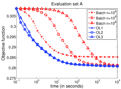
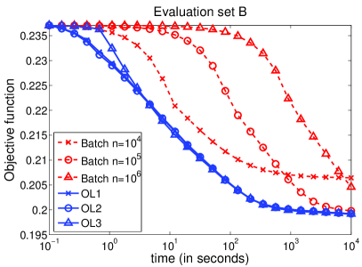
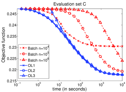
The left column of Figure 1 compares the online and batch settings of our implementation. The full training set consists of $10^{6}$ samples. The online version of our algorithm draws samples from the entire set, and we have run its batch version on the full data set as well as subsets of size $10^{4}$ and $10^{5}$ (see Figure 1). The online setting systematically outperforms its batch counterpart for every training set size and desired precision. We use a logarithmic scale for the computation time, which shows that in many situations, the difference in performance can be dramatic. Similar experiments have given similar results on smaller data sets. Our algorithm uses all the speed-ups from Section 3.4. The parameter $\rho$ was chosen by trying the values $0,5,10,15,20,25$, and $t_{0}$ by trying different powers of $10$. We have selected $(t_{0}=0.001,\rho=15)$, which has given the best performance in terms of objective function evaluated on the training set for the three data sets. We have plotted three curves for our method: OL1 corresponds to the optimal setting $(t_{0}=0.001,\rho=15)$. Even though tuning two parameters might seem cumbersome, we have plotted two other curves showing that, on the contrary, our method is very easy to use. The curve OL2, corresponding to the setting $(t_{0}=0.001,\rho=10)$, is very difficult to distinguish from the first curve and we have observed a similar behavior with the setting $(t_{0}=0.001,\rho=20)$. showing that our method is robust to the choice of the parameter $\rho$. We have also observed that the parameter $\rho$ is useful for large data sets only. When using smaller ones ($n\leq 100,000$), it did not bring any benefit.

Moreover, the curve OL3 is obtained without using a tuned parameter $t_{0}$—that is, $\rho=15$ and $t_{0}=0$, and shows that its influence is very limited since very good results are obtained without using it. On the other hand, we have observed that using a parameter $t_{0}$ too big, could slightly slow down our algorithm during the first epoch (cycle on the training set).

Figure 1: Left: Comparison between our method and the batch approach for dictionary learning. Right: Comparison between our method and stochastic gradient descent. The results are reported for three data sets as a function of computation time on a logarithmic scale. Note that the times of computation that are less than $0.1s$ are not reported. See text for details.

6.1.2 Comparison with Stochastic Gradient Descent

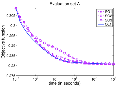
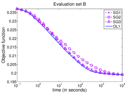
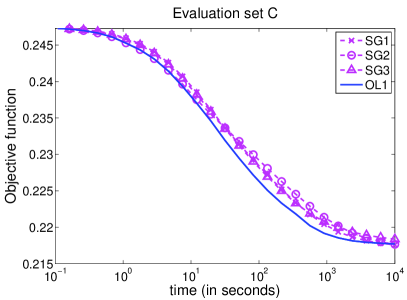
Our experiments have shown that obtaining good performance with stochastic gradient descent requires using both the mini-batch heuristic and carefully choosing a learning rate of the form $a/(\eta t+b)$. To give the fairest comparison possible, we have thus optimized these parameters. As for our algorithm, sampling $\eta$ values among powers of 2 (as before) has shown that $\eta=512$ was a good value and gives a significant better performance than $\eta=1$.

In an earlier version of this work (Mairal et al., 2009a), we have proposed a strategy for our method which does not require any parameter tuning except the mini-batch $\eta$ and compared it with the stochastic gradient descent algorithm (SGD) with a learning rate of the form $a/(\eta t)$. While our method has improved in performance using the new parameter $\rho$, SGD has also proven to provide much better results when using a learning rate of the form $a/(\eta t+b)$ instead of $a/(\eta t)$, at the cost of an extra parameter $b$ to tune. Using the learning rate $a/(\eta t)$ with a high value for $a$ results indeed in too large initial steps of the algorithm increasing dramatically the value of the objective function, and a small value of $a$ leads to bad asymptotic results, while a learning rate of the form $a/(\eta t+b)$ is a good compromise.

We have tried different powers of $10$ for $a$ and $b$. First selected the couple ($a=100,000,b=100,000$) and then refined it, trying the values $100,000\times 2^{i}$ for $i=-3,\ldots,3$. Finally, we have selected $(a=200,000,b=400,000)$. As shown on the right column of Figure 1, this setting represented by the curve SG1 leads to similar results as our method. The curve SG2 corresponds to the parameters $(a=400,000,b=400,000)$ and shows that increasing slightly the parameter $a$ makes the curves worse than the others during the first iterations (see for instance the curve between $1$ and $10^{2}$ seconds for data set A), but still lead to good asymptotic results. The curve SG3 corresponds to a situation where $a$ and $b$ are slightly too small $(a=50,000,b=100,000)$. It is as good as SG1 for data sets A and B, but asymptotically slightly below the others for data set C. All the curves are obtained as the average of three experiments with different initializations. Interestingly, even though the problem is not convex, the different initializations have led to very similar values of the objective function and the variance of the experiments was always insignificant after $10$ seconds of computations.

6.2 Non Negative Matrix Factorization and Non Negative Sparse Coding

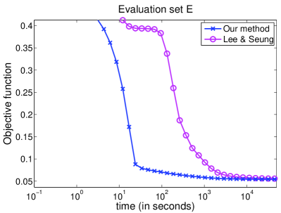
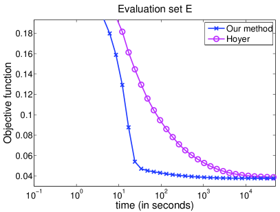
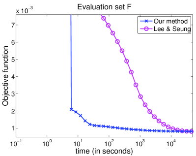
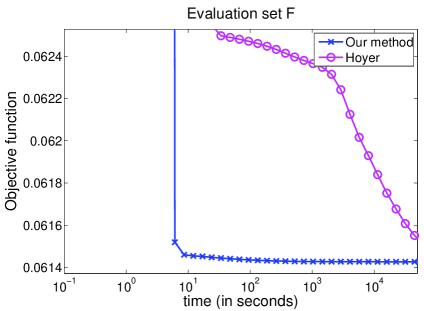
In this section, we compare our method with the classical algorithm of Lee and Seung (2001) for NMF and the non-negative sparse coding algorithm of Hoyer (2002) for NNSC. The experiments have been carried out on three data sets with different sizes:

• Data set D is composed of $n=2,429$ face images of size $m=19\times 19$ pixels from the the MIT-CBCL Face Database $\#1$ (Sung, 1996).

• Data set E is composed of $n=2,414$ face images of size $m=192\times 168$ pixels from the Extended Yale B Database (Georghiades et al., 2001; Lee et al., 2005).

• Data set F is composed of $n=100,000$ natural image patches of size $m=16\times 16$ pixels from the Pascal VOC’06 image database (Everingham et al., 2006).

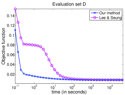
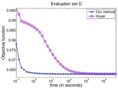
We have used the Matlab implementations of NMF and NNSC of P. Hoyer, which are freely available at http://www.cs.helsinki.fi/u/phoyer/software.html. Even though our C++ implementation has a built-in advantage in terms of speed over these Matlab implementations, most of the computational time of NMF and NNSC is spent on large matrix multiplications, which are typically well optimized in Matlab. All the experiments have been run for simplicity on a single-CPU, single-core 2.4GHz machine, without using the parameters $\rho$ and $t_{0}$ presented in Section 3.4—that is, $\rho=0$ and $t_{0}=0$. As in Section 6.1, a minibatch of size $\eta=512$ is chosen. Following the original experiment of Lee and Seung (2001) on data set D, we have chosen to learn $k=49$ basis vectors for the face images data sets D and E, and we have chosen $k=64$ for data set F. Each input vector is normalized to have unit $\ell_{2}$-norm.

The experiments we present in this section compare the value of the objective function on the data sets obtained with the different algorithms as a function of the computation time. Since our algorithm learns the matrix ${\mathbf{D}}$ but does not provide the matrix ${\boldsymbol{\alpha}}$, the computation times reported for our approach include two steps: First, we run our algorithm to obtain ${\mathbf{D}}$. Second, we run one sparse coding step over all the input vectors to obtain ${\boldsymbol{\alpha}}$. Figure 2 presents the results for NMF and NNSC. The gradient step for the algorithm of Hoyer (2002) was optimized for the best performance and $\lambda$ was set to $\frac{1}{\sqrt{m}}$. Both ${\mathbf{D}}$ and ${\boldsymbol{\alpha}}$ were initialized randomly. The values reported are those obtained for more than $0.1$s of computation. Since the random initialization provides an objective value which is by far greater than the value obtained at convergence, the curves are all truncated to present significant objective values. All the results are obtained using the average of 3 experiments with different initializations. As shown on Figure 2, our algorithm provides a significant improvement in terms of speed compared to the other tested methods, even though the results for NMF and NNSC could be improved a bit using a C++ implementation.

Figure 2: Left: Comparison between our method and the approach of Lee and Seung (2001) for NMF. Right: Comparison between our method and the approach of Hoyer (2002) for NNSC. The value of the objective function is reported for three data sets as a function of computation time on a logarithmic scale.

6.3 Sparse Principal Component Analysis

We present here the application of our method addressing SPCA with various types of data: faces, natural image patches, and genomic data.

6.3.1 Faces and Natural Patches

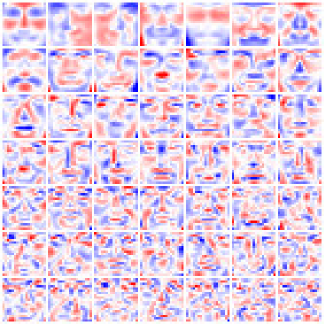
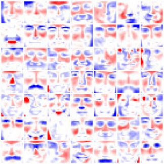
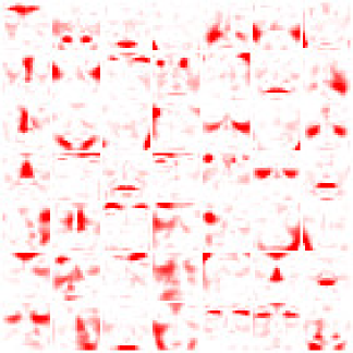
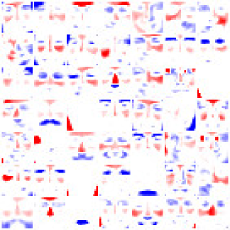
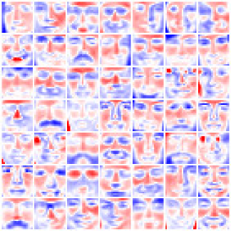
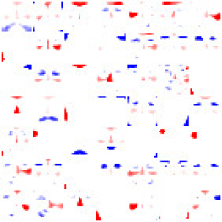
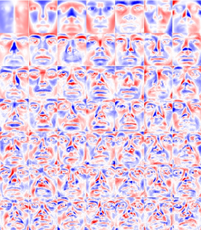
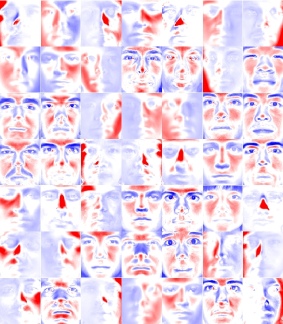
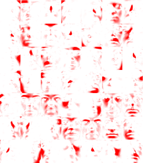
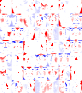
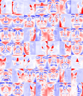
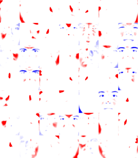
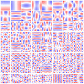
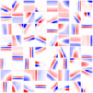
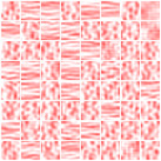
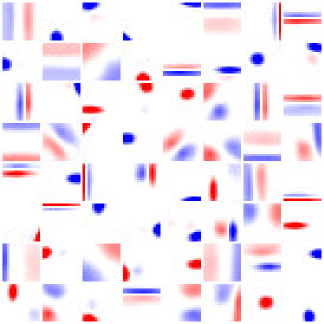
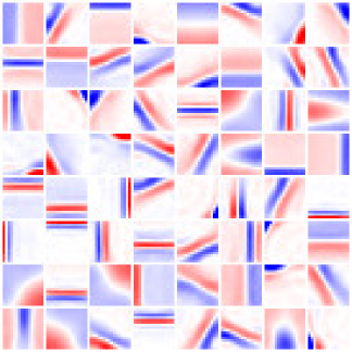
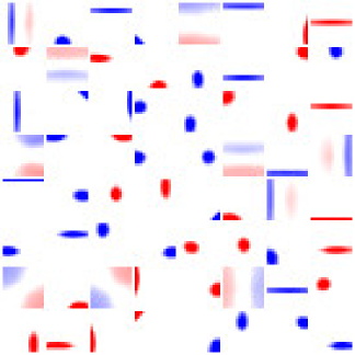
In this section, we compare qualitatively the results obtained by PCA, NMF, our dictionary learning and our sparse principal component analysis algorithm on the data sets used in Section 6.2. For dictionary learning, PCA and SPCA, the input vectors are first centered and normalized to have a unit norm. Visual results are presented on figures 3, 4 and 5, respectively for the data sets D, E and F. The parameter $\lambda$ for dictionary learning and SPCA was set so that the decomposition of each input signal has approximately $10$ nonzero coefficients. The results for SPCA are presented for various values of the parameter $\gamma$, yielding different levels of sparsity. The scalar $\tau$ indicates the percentage of nonzero values of the dictionary.

Each image is composed of $k$ small images each representing one learned feature vector. Negative values are blue, positive values are red and the zero values are represented in white. Confirming earlier observations from Lee and Seung (2001), PCA systematically produces features spread out over the images, whereas NMF produces more localized features on the face databases D and E. However, neither PCA, nor NMF are able to learn localized features on the set of natural patches F. On the other hand, the dictionary learning technique is able to learn localized features on data set F, and SPCA is the only tested method that allows controlling the level of sparsity among the learned matrices.

(a) PCA

(b) SPCA, $\tau=70\%$

(c) NMF

(d) SPCA, $\tau=30\%$

(e) Dictionary Learning

(f) SPCA, $\tau=10\%$

Figure 3: Results obtained by PCA, NMF, dictionary learning, SPCA for data set D.

(a) PCA

(b) SPCA, $\tau=70\%$

(c) NMF

(d) SPCA, $\tau=30\%$

(e) Dictionary Learning

(f) SPCA, $\tau=10\%$

Figure 4: Results obtained by PCA, NMF, dictionary learning, SPCA for data set E.

(a) PCA

(b) SPCA, $\tau=70\%$

(c) NMF

(d) SPCA, $\tau=30\%$

(e) Dictionary Learning

(f) SPCA, $\tau=10\%$

Figure 5: Results obtained by PCA, NMF, dictionary learning, SPCA for data set F.

6.3.2 Genomic Data

This experiment follows Witten et al. (2009) and demonstrates that our matrix decomposition technique can be used for analyzing genomic data. Gene expression measurements and DNA copy number changes (comparative genomic hybridization CGH) are two popular types of data in genomic research, which can be used to characterize a set of abnormal tissue samples for instance. When these two types of data are available, a recent line of research tries to analyze the correlation between them—that is, to determine sets of expression genes which are correlated with sets of chromosomal gains or losses (see Witten et al., 2009 and references therein). Let us suppose that for $n$ tissue samples, we have a matrix ${\mathbf{X}}$ in ${\mathbb{R}}^{n\times p}$ of gene expression measurements and a matrix ${\mathbf{Y}}$ in ${\mathbb{R}}^{n\times q}$ of CGH measurements. In order to analyze the correlation between these two sets of data, recent works have suggested the use of canonical correlation analysis (Hotelling, 1936), which solves

$$\min_{{\mathbf{u}}\in{\mathbb{R}}^{p},{\mathbf{v}}\in{\mathbb{R}}^{q}}\operatorname{cov}({\mathbf{X}}{\mathbf{u}},{\mathbf{Y}}{\mathbf{v}})~{}~{}\text{s.t.}~{}~{}||{\mathbf{X}}{\mathbf{u}}||_{2}\leq 1~{}~{}\text{and}~{}~{}||{\mathbf{Y}}{\mathbf{v}}||_{2}\leq 1.$$

When ${\mathbf{X}}$ and ${\mathbf{Y}}$ are centered and normalized, it has been further shown that with this type of data, good results can be obtained by treating the covariance matrices ${\mathbf{X}}^{T}{\mathbf{X}}$ and ${\mathbf{Y}}^{T}{\mathbf{Y}}$ as diagonal, leading to a rank-one matrix decomposition problem

$$\min_{{\mathbf{u}}\in{\mathbb{R}}^{p},{\mathbf{v}}\in{\mathbb{R}}^{q}}||{\mathbf{X}}^{T}{\mathbf{Y}}-{\mathbf{u}}{\mathbf{v}}^{T}||_{F}^{2}~{}~{}\text{s.t.}~{}~{}||{\mathbf{u}}||_{2}\leq 1,~{}~{}\text{and}~{}~{}||{\mathbf{v}}||_{2}\leq 1.$$

Furthermore, as shown by Witten et al. (2009), this method can benefit from sparse regularizers such as the $\ell_{1}$ norm for the gene expression measurements and a fused lasso for the CGH arrays, which are classical choices used for these data. The formulation we have chosen is slightly different from the one used by Witten et al. (2009) and can be addressed using our algorithm:

$$\min_{{\mathbf{u}}\in{\mathbb{R}}^{p},{\mathbf{v}}\in{\mathbb{R}}^{q}}||{\mathbf{Y}}^{T}{\mathbf{X}}-{\mathbf{v}}{\mathbf{u}}^{T}||_{F}^{2}+\lambda||{\mathbf{u}}||_{2}~{}~{}\text{s.t.}~{}~{}||{\mathbf{v}}||_{2}^{2}+\gamma_{1}||{\mathbf{v}}||_{1}+\gamma_{2}\operatorname{FL}({\mathbf{v}})\leq 1.$$ (17)

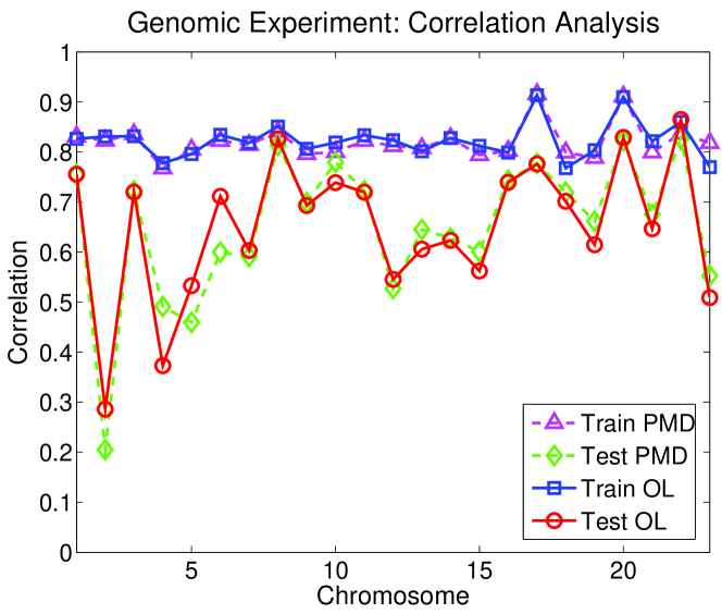
In order to assess the effectivity of our method, we have conducted the same experiment as Witten et al. (2009) using the breast cancer data set described by Chin et al. (2006), consisting of $q=2,148$ gene expression measurements and $p=16,962$ CGH measurements for $n=89$ tissue samples. The matrix decomposition problem of Eq. (17) was addressed once for each of the $23$ chromosomes, using each time the CGH data available for the corresponding chromosome, and the gene expression of all genes. Following the original choice of Witten et al. (2009), we have selected a regularization parameter $\lambda$ resulting in about $25$ non-zero coefficients in ${\mathbf{u}}$, and selected $\gamma_{1}=\gamma_{2}=1$, which results in sparse and piecewise-constant vectors ${\mathbf{v}}$. The original matrices $({\mathbf{X}},{\mathbf{Y}})$ are divided into a training set $({\mathbf{X}}_{tr},{\mathbf{Y}}_{tr})$ formed with $3/4$ of the $n$ samples, keeping the rest $({\mathbf{X}}_{te},{\mathbf{Y}}_{te})$ for testing. This experiment is repeated for $10$ random splits, for each chromosome a couple of factors $({\mathbf{u}},{\mathbf{v}})$ are computed, and the correlations $\operatorname{corr}({\mathbf{X}}_{tr}{\mathbf{u}},{\mathbf{Y}}_{tr}{\mathbf{v}})$ and $\operatorname{corr}({\mathbf{X}}_{te}{\mathbf{u}},{\mathbf{Y}}_{te}{\mathbf{v}})$ are reported on Figure 6. The average standard deviation of the experiments results was $0.0339$ for the training set and $0.1391$ for the test set.

Comparing with the original curves reported by Witten et al. (2009) for their penalized matrix decomposition (PMD) algorithm, our method exhibits in general a performance similar as PMD. Nevertheless, the purpose of this section is more to demonstrate that our method can be used with genomic data than comparing it carefully with PMD. To draw substantial conclusions about the performance of both methods, more experiments would of course be needed.

Figure 6: SPCA was applied to the covariance matrix obtained from the breast cancer data (Chin et al., 2006). A fused lasso regularization is used for the CGH data. $3/4$ of the $n$ samples are used as a training set, keeping the rest for testing. Average correlations from $10$ random splits are reported for each of the $23$ chromosomes, for PMD (Witten et al., 2009) and our method denoted by OL.

6.4 Application to Large-Scale Image Processing

We demonstrate in this section that our algorithm can be used for a difficult large-scale image processing task, namely, removing the text (inpainting) from the damaged $12$-Megapixel image of Figure 7. Using a multi-threaded version of our implementation, we have learned a dictionary with $256$ elements from the roughly $7\times 10^{6}$ undamaged $12\times 12$ color patches in the image with two epochs in about $8$ minutes on a 2.4GHz machine with eight cores. Once the dictionary has been learned, the text is removed using the sparse coding technique for inpainting of Mairal et al. (2008b). Our intent here is of course not to evaluate our learning procedure in inpainting tasks, which would require a thorough comparison with state-the-art techniques on standard data sets. Instead, we just wish to demonstrate that it can indeed be applied to a realistic, non-trivial image processing task on a large image. Indeed, to the best of our knowledge, this is the first time that dictionary learning is used for image restoration on such large-scale data. For comparison, the dictionaries used for inpainting in Mairal et al. (2008b) are learned (in batch mode) on 200,000 patches only.

Figure 7: Inpainting example on a $12$-Megapixel image. Top: Damaged and restored images. Bottom: Zooming on the damaged and restored images. Note that the pictures presented here have been scaled down for display. (Best seen in color).

7 Conclusion

We have introduced in this paper a new stochastic online algorithm for learning dictionaries adapted to sparse coding tasks, and proven its convergence. Experiments demonstrate that it is significantly faster than batch alternatives such as Engan et al. (1999), Aharon et al. (2006) and Lee et al. (2007) on large data sets that may contain millions of training examples, yet it does not require a careful learning rate tuning like regular stochastic gradient descent methods. Moreover, we have extended it to other matrix factorization problems such as non negative matrix factorization, and we have proposed a formulation for sparse principal component analysis which can be solved efficiently using our method. Our approach has already shown to be useful for image restoration tasks such as denoising (Mairal et al., 2009c); more experiments are of course needed to better assess its promise in bioinformatics and signal processing. Beyond this, we plan to use the proposed learning framework for sparse coding in computationally demanding video restoration tasks (Protter and Elad, 2009), with dynamic data sets whose size is not fixed, and extending this framework to different loss functions (Mairal et al., 2009b) to address discriminative tasks such as image classification, which are more sensitive to overfitting than reconstructive ones.

Acknowledgments

This paper was supported in part by ANR under grant MGA ANR-07-BLAN-0311. The work of Guillermo Sapiro is partially supported by ONR, NGA, NSF, ARO, and DARPA. The authors would like to thank Sylvain Arlot, Léon Bottou, Jean-Philippe Vert, and the members of the Willow project-team for helpful discussions, and Daniela Witten for providing us with her code to generate the curves of Figure 6.

A Theorems and Useful Lemmas

We provide in this section a few theorems and lemmas from the optimization and probability literature, which are used in this paper.

Theorem 1

[Corollary of Theorem 4.1 from Bonnans and Shapiro (1998), due to Danskin (1967)].
Let $f:{\mathbb{R}}^{p}\times{\mathbb{R}}^{q}\to{\mathbb{R}}$. Suppose that for all ${\mathbf{x}}\in{\mathbb{R}}^{p}$ the function $f({\mathbf{x}},.)$ is differentiable, and that $f$ and $\nabla_{{\mathbf{u}}}f({\mathbf{x}},{\mathbf{u}})$ the derivative of $f({\mathbf{x}},.)$ are continuous on ${\mathbb{R}}^{p}\times{\mathbb{R}}^{q}$. Let $v({\mathbf{u}})$ be the optimal value function $v({\mathbf{u}})=\min_{{\mathbf{x}}\in C}f({\mathbf{x}},{\mathbf{u}})$, where $C$ is a compact subset of ${\mathbb{R}}^{p}$. Then $v({\mathbf{u}})$ is directionally differentiable. Furthermore, if for ${\mathbf{u}}_{0}\in{\mathbb{R}}^{q}$, $f(.,{\mathbf{u}}_{0})$ has a unique minimizer ${\mathbf{x}}_{0}$ then $v({\mathbf{u}})$ is differentiable in ${\mathbf{u}}_{0}$ and $\nabla_{{\mathbf{u}}}v({\mathbf{u}}_{0})=\nabla_{{\mathbf{u}}}f({\mathbf{x}}_{0},{\mathbf{u}}_{0})$.

Theorem 2

[Sufficient condition of convergence for a stochastic process, see Bottou (1998) and references therein (Métivier, 1983; Fisk, 1965)].
Let ($\Omega$,$\mathcal{F}$,$P$) be a measurable probability space, $u_{t}$, for $t\geq 0$, be the realization of a stochastic process and ${\mathcal{F}}_{t}$ be the filtration determined by the past information at time $t$. Let

$$\delta_{t}=\left\{\begin{array}[]{ll}1&~{}~{}\text{if}~{}~{}{\mathbb{E}}[u_{t+1}-u_{t}|{\mathcal{F}}_{t}]>0,\\ 0&~{}~{}\text{otherwise.}\end{array}\right.$$

If for all $t$, $u_{t}\geq 0$ and $\sum_{t=1}^{\infty}{\mathbb{E}}[\delta_{t}(u_{t+1}-u_{t})]<\infty$, then $u_{t}$ is a quasi-martingale and converges almost surely. Moreover,

$$\sum_{t=1}^{\infty}|{\mathbb{E}}[u_{t+1}-u_{t}|{\mathcal{F}}_{t}]|<+\infty\text{~{}~{}a.s.}$$

Lemma 2

[A corollary of Donsker theorem see Van der Vaart, 1998, chap. 19.2, lemma 19.36 and example 19.7].
Let $F=\{f_{\theta}:\chi\to{\mathbb{R}},\theta\in\Theta\}$ be a set of measurable functions indexed by a bounded subset $\Theta$ of ${\mathbb{R}}^{d}$. Suppose that there exists a constant $K$ such that

$$|f_{\theta_{1}}(x)-f_{\theta_{2}}(x)|\leq K||\theta_{1}-\theta_{2}||_{2},$$

for every $\theta_{1}$ and $\theta_{2}$ in $\Theta$ and $x$ in $\chi$. Then, $F$ is P-Donsker (see Van der Vaart, 1998, chap. 19.2). For any $f$ in $F$, Let us define ${\mathbb{P}}_{n}f$, ${\mathbb{P}}f$ and ${\mathbb{G}}_{n}f$ as

$${\mathbb{P}}_{n}f=\frac{1}{n}\sum_{i=1}^{n}f(X_{i}),~{}~{}~{}~{}{\mathbb{P}}f={\mathbb{E}}_{X}[f(X)],~{}~{}~{}~{}{\mathbb{G}}_{n}f=\sqrt{n}({\mathbb{P}}_{n}f-{\mathbb{P}}f).$$

Let us also suppose that for all $f$, ${\mathbb{P}}f^{2}<\delta^{2}$ and $||f||_{\infty}<M$ and that the random elements $X_{1},X_{2},\ldots$ are Borel-measurable. Then, we have

$${\mathbb{E}}_{P}||{\mathbb{G}}_{n}||_{F}={O}(1),$$

where $||{\mathbb{G}}_{n}||_{F}=\sup_{f\in F}|{\mathbb{G}}_{n}f|$. For a more general variant of this lemma and additional explanations and examples, see Van der Vaart (1998).

Lemma 3

[A simple lemma on positive converging sums].
Let $a_{n}$, $b_{n}$ be two real sequences such that for all $n$, $a_{n}\geq 0,b_{n}\geq 0$, $\sum_{n=1}^{\infty}a_{n}=\infty$, $\sum_{n=1}^{\infty}a_{n}b_{n}<\infty$, $\exists K>0~{}~{}\text{s.t.}~{}~{}|b_{n+1}-b_{n}|<Ka_{n}$. Then, $\lim_{n\to+\infty}b_{n}=0$.

Proof.  The proof is similar to Bertsekas (1999, prop 1.2.4).  

B Efficient Projections Algorithms

In this section, we address the problem of efficiently projecting a vector onto two sets of constraints, which allows us to extend our algorithm to various other formulations.

B.1 A Linear-time Projection on the Elastic-Net Constraint

Let ${\mathbf{b}}$ be a vector of ${\mathbb{R}}^{m}$. We consider the problem of projecting this vector onto the elastic-net constraint set:

$$\min_{{\mathbf{u}}\in{\mathbb{R}}^{m}}\frac{1}{2}||{\mathbf{b}}-{\mathbf{u}}||_{2}^{2}~{}~{}\text{s.t.}~{}~{}||{\mathbf{u}}||_{1}+\frac{\gamma}{2}||{\mathbf{u}}||_{2}^{2}\leq\tau.$$ (18)

To solve efficiently the case $\gamma>0$, we propose Algorithm 3, which extends Maculan and de Paula (1989) and Duchi et al. (2008), and the following lemma which shows that it solves our problem.

Lemma 4

[Projection onto the elastic-net constraint set].
For ${\mathbf{b}}$ in ${\mathbb{R}}^{m}$, $\gamma\geq 0$ and $\tau>0$, Algorithm 3 solves Eq. (18).

Proof.  First, if ${\mathbf{b}}$ is a feasible point of (18), then ${\mathbf{b}}$ is a solution. We suppose therefore that it is not the case—that is,$||{\mathbf{b}}||_{1}+\frac{\gamma}{2}||{\mathbf{b}}||_{2}^{2}>\tau$. Let us define the Lagrangian of (18)

$${\mathcal{L}}({\mathbf{u}},\lambda)=\frac{1}{2}||{\mathbf{b}}-{\mathbf{u}}||_{2}^{2}+\lambda\big{(}||{\mathbf{u}}||_{1}+\frac{\gamma}{2}||{\mathbf{u}}||_{2}^{2}-\tau\big{)}.$$

For a fixed $\lambda$, minimizing the Lagrangian with respect to ${\mathbf{u}}$ admits a closed-form solution ${\mathbf{u}}^{\star}(\lambda)$, and a simple calculation shows that, for all $j$,

$${\mathbf{u}}^{\star}(\lambda)[j]=\frac{\operatorname{sign}({\mathbf{b}}[j])(|{\mathbf{b}}[j]|-\lambda)^{+}}{1+\lambda\gamma}.$$

Eq. (18) is a convex optimization problem. Since Slater’s conditions are verified and strong duality holds, it is equivalent to the dual problem

$$\max_{\lambda\geq 0}{\mathcal{L}}({\mathbf{u}}^{\star}(\lambda),\lambda).$$

Since $\lambda=0$ is not a solution, denoting by $\lambda^{\star}$ the solution, the complementary slackness condition implies that

$$||{\mathbf{u}}^{\star}(\lambda^{\star})||_{1}+\frac{\gamma}{2}||{\mathbf{u}}^{\star}(\lambda^{\star})||_{2}^{2}=\tau.$$ (19)

Using the closed form of ${\mathbf{u}}^{\star}(\lambda)$ is possible to show that the function $\lambda\to||{\mathbf{u}}^{\star}(\lambda)||_{1}+\frac{\gamma}{2}||{\mathbf{u}}^{\star}(\lambda)||_{2}^{2}$, is strictly decreasing with $\lambda$ and thus Eq. (19) is a necessary and sufficient condition of optimality for $\lambda$. After a short calculation, one can show that this optimality condition is equivalent to

$$\frac{1}{(1+\lambda\gamma)^{2}}\sum_{j\in S(\lambda)}\Big{(}|{\mathbf{b}}[j]|+\frac{\gamma}{2}|{\mathbf{b}}[j]|^{2}-\lambda\big{(}1+\frac{\gamma\lambda}{2}\big{)}\Big{)}=\tau,$$

where $S(\lambda)=\{j~{}~{}\text{s.t.}~{}~{}|{\mathbf{b}}[j]|\geq\lambda\}$. Suppose that $S(\lambda^{\star})$ is known, then $\lambda^{\star}$ can be computed in closed-form. To find $S(\lambda^{\star})$, it is then sufficient to find the index $k$ such that $S(\lambda^{\star})=S(|{\mathbf{b}}[k]|)$, which is the solution of

$$\max_{k\in\{1,\ldots,m\}}|{\mathbf{b}}[k]|~{}~{}\text{s.t.}~{}~{}\frac{1}{(1+|{\mathbf{b}}[k]|\gamma)^{2}}\sum_{j\in S(|{\mathbf{b}}[k]|)}\Big{(}|{\mathbf{b}}[j]|+\frac{\gamma}{2}|{\mathbf{b}}[j]|^{2}-|{\mathbf{b}}[k]|\big{(}1+\frac{\gamma|{\mathbf{b}}[k]|}{2}\big{)}\Big{)}<\tau.$$

Lines 4 to 14 of Algorithm 3 are a modification of Duchi et al. (2008) to address this problem. A similar proof as Duchi et al. (2008) shows the convergence to the solution of this optimization problem in ${O}(m)$ in the average case, and lines 15 to 18 of Algorithm 3) compute $\lambda^{\star}$ after that $S(\lambda^{\star})$ has been identified. Note that setting $\gamma$ to $0$ leads exactly to the algorithm of Duchi et al. (2008).  

Algorithm 3 Efficient projection on the elastic-net constraint.

0:  $\tau\in{\mathbb{R}}$; $\gamma\in{\mathbb{R}}$; ${\mathbf{b}}\in{\mathbb{R}}^{m}$;

1:  if $||{\mathbf{b}}||_{1}+\frac{\gamma}{2}||{\mathbf{b}}||_{2}^{2}\leq\tau$ then

2:     return  ${\mathbf{u}}\leftarrow{\mathbf{b}}$.

3:  else

4:     $U\leftarrow\{1,\ldots,m\}$; $s\leftarrow 0$; $\rho\leftarrow 0$.

5:     while $U\neq\emptyset$ do

6:        Pick $k\in U$ at random.

7:        Partition $U$:

$$\begin{split}G&=\{j\in U~{}~{}\text{s.t.}~{}~{}|{\mathbf{b}}[j]|\geq|{\mathbf{b}}[k]|\},\\ L&=\{j\in U~{}~{}\text{s.t.}~{}~{}|{\mathbf{b}}[j]|<|{\mathbf{b}}[k]|\}.\\ \end{split}$$

8:        $\Delta\rho\leftarrow|G|$; $\Delta s\leftarrow\sum_{j\in G}|{\mathbf{b}}[j]|+\frac{\gamma}{2}|{\mathbf{b}}[j]|^{2}$.

9:        if  $s+\Delta s-(\rho+\Delta\rho)(1+\frac{\gamma}{2}|{\mathbf{b}}[k]|)|{\mathbf{b}}[k]|<\tau(1+\gamma|{\mathbf{b}}[k]|)^{2}$ then

10:           $s\leftarrow s+\Delta s;\rho\leftarrow\Delta\rho;U\leftarrow L$.

11:        else

12:           $U\leftarrow G\setminus\{k\}$.

13:        end if

14:     end while

15:     $a\leftarrow\gamma^{2}\tau+\frac{\gamma}{2}\rho$,

16:     $b\leftarrow 2\gamma\tau+\rho$,

17:     $c\leftarrow\tau-s$,

18:     $\lambda\leftarrow\frac{-b+\sqrt{b^{2}-4ac}}{2a}$

19:     

$$\forall j=1,\ldots,n,{\mathbf{u}}[j]\leftarrow\frac{\operatorname{sign}({\mathbf{b}}[j])(|{\mathbf{b}}[j]|-\lambda)^{+}}{1+\lambda\gamma}$$

20:     return  ${\mathbf{u}}$.

21:  end if

As for the dictionary learning problem, a simple modification to Algorithm 3 allows us to handle the non-negative case, replacing the scalars $|{\mathbf{b}}[j]|$ by $\max({\mathbf{b}}[j],0)$ in the algorithm.

B.2 A Homotopy Method for Solving the Fused Lasso Signal Approximation

Let ${\mathbf{b}}$ be a vector of ${\mathbb{R}}^{m}$. We define, following Friedman et al. (2007), the fused lasso signal approximation problem ${\mathcal{P}}(\gamma_{1},\gamma_{2},\gamma_{3})$:

$$\min_{{\mathbf{u}}\in{\mathbb{R}}^{m}}\frac{1}{2}||{\mathbf{b}}-{\mathbf{u}}||_{2}^{2}+\gamma_{1}||{\mathbf{u}}||_{1}+\gamma_{2}\operatorname{FL}({\mathbf{u}})+\frac{\gamma_{3}}{2}||{\mathbf{u}}||_{2}^{2},$$ (20)

the only difference with Friedman et al. (2007) being the addition of the last quadratic term. The method we propose to this problem is a homotopy, which solves ${\mathcal{P}}(\tau\gamma_{1},\tau\gamma_{2},\tau\gamma_{3})$ for all possible values of $\tau$. In particular, for all $\varepsilon$, it provides the solution of the constrained problem

$$\min_{{\mathbf{u}}\in{\mathbb{R}}^{m}}\frac{1}{2}||{\mathbf{b}}-{\mathbf{u}}||_{2}^{2}~{}~{}\text{s.t.}~{}~{}\gamma_{1}||{\mathbf{u}}||_{1}+\gamma_{2}\operatorname{FL}({\mathbf{u}})+\frac{\gamma_{3}}{2}||{\mathbf{u}}||_{2}^{2}\leq\varepsilon.$$ (21)

The algorithm relies on the following lemma

Lemma 5

Let ${\mathbf{u}}^{\star}(\gamma_{1},\gamma_{2},\gamma_{3})$ be the solution of Eq. (20), for specific values of $\gamma_{1},\gamma_{2},\gamma_{3}$. Then

• ${\mathbf{u}}^{\star}(\gamma_{1},\gamma_{2},\gamma_{3})=\frac{1}{1+\gamma_{3}}{\mathbf{u}}^{\star}(\gamma_{1},\gamma_{2},0)$.

• For all $i$, ${\mathbf{u}}^{\star}(\gamma_{1},\gamma_{2},0)[i]=\operatorname{sign}({\mathbf{u}}^{\star}(0,\gamma_{2},0)[i])\max(|{\mathbf{u}}^{\star}(0,\gamma_{2},0)[i]|-\lambda_{1},0)$—that is, ${\mathbf{u}}^{\star}(\gamma_{1},\gamma_{2},0)$ can be obtained by soft thresholding of ${\mathbf{u}}^{\star}(0,\gamma_{2},0)$.

The first point can be shown by short calculation. The second one is proven in Friedman et al. (2007) by considering subgradient optimality conditions. This lemma shows that if one knows the solution of ${\mathcal{P}}(0,\gamma_{2},0)$, then ${\mathcal{P}}(\gamma_{1},\gamma_{2},\gamma_{3})$ can be obtained in linear time.

It is therefore natural to consider the simplified problem

$$\min_{{\mathbf{u}}\in{\mathbb{R}}^{m}}\frac{1}{2}||{\mathbf{b}}-{\mathbf{u}}||_{2}^{2}+\gamma_{2}\operatorname{FL}({\mathbf{u}}).$$ (22)

With the change of variable ${\mathbf{v}}[1]={\mathbf{u}}[1]$ and ${\mathbf{v}}[i]={\mathbf{u}}[i]-{\mathbf{u}}[i-1]$ for $i>1$, this problem can be recast as a weighted Lasso

$$\min_{{\mathbf{v}}\in{\mathbb{R}}^{m}}\frac{1}{2}||{\mathbf{b}}-{\mathbf{D}}{\mathbf{v}}||_{2}^{2}+\sum_{i=1}^{m}w_{i}|{\mathbf{v}}[i]|,$$ (23)

where $w_{1}=0$ and $w_{i}=\gamma_{2}$ for $i>1$, and ${\mathbf{D}}[i,j]=1$ if $i\geq j$ and $0$ otherwise. We propose to use LARS (Efron et al., 2004) and exploit the specific structure of the matrix ${\mathbf{D}}$ to make this approach efficient, by noticing that:

• For a vector ${\mathbf{w}}$ in ${\mathbb{R}}^{m}$, computing ${\mathbf{e}}={\mathbf{D}}{\mathbf{w}}$ requires $O(m)$ operations instead of $O(m^{2})$, by using the recursive formula ${\mathbf{e}}[1]={\mathbf{w}}[1]$, ${\mathbf{e}}[i+1]={\mathbf{w}}[i]+{\mathbf{e}}[i]$.

• For a vector ${\mathbf{w}}$ in ${\mathbb{R}}^{n}$, computing ${\mathbf{e}}={\mathbf{D}}^{T}{\mathbf{w}}$ requires $O(m)$ operations instead of $O(m^{2})$, by using the recursive formula ${\mathbf{e}}[n]={\mathbf{w}}[n]$, ${\mathbf{e}}[i-1]={\mathbf{w}}[i-1]+{\mathbf{e}}[i]$.

• Let ${\boldsymbol{\Gamma}}=\{a_{1},\ldots,a_{p}\}$ be an active set and suppose $a_{1}<\ldots<a_{p}$. Then $({\mathbf{D}}_{\boldsymbol{\Gamma}}^{T}{\mathbf{D}}_{\boldsymbol{\Gamma}})^{-1}$ admits the closed form value

  $$({\mathbf{D}}_{\boldsymbol{\Gamma}}^{T}{\mathbf{D}}_{\boldsymbol{\Gamma}})^{-1}=\left(\begin{array}[]{cccccc}c_{1}&-c_{1}&0&\ldots&0&0\\ -c_{1}&c_{1}+c_{2}&-c_{2}&\ldots&0&0\\ 0&-c_{2}&c_{2}+c_{3}&\ldots&0&0\\ \vdots&\vdots&\vdots&\ddots&\vdots&\vdots\\ 0&0&0&\ldots&c_{p-2}+c_{p-1}&-c_{p-1}\\ 0&0&0&\ldots&-c_{p-1}&c_{p-1}+c_{p}\end{array}\right),$$

  where $c_{p}=\frac{1}{n+1-a_{p}}$ and $c_{i}=\frac{1}{a_{i+1}-a_{i}}$ for $i<p$.

This allows the implementation of this homotopy method without using matrix inversion or Cholesky factorization, solving Eq. (23) in $O(ms)$ operations, where $s$ is the number of non-zero values of the optimal solution ${\mathbf{v}}$.

Adapting this method for solving Eq. (21) requires following the regularization path of the problems ${\mathcal{P}}(0,\tau\gamma_{2},0)$ for all values of $\tau$, which provides as well the regularization path of the problem ${\mathcal{P}}(\tau\lambda_{1},\tau\lambda_{2},\tau\lambda_{3})$ and stops whenever the constraint becomes unsatisfied. This procedure still requires $O(ms)$ operations.

Note that in the case $\gamma_{1}=0$ and $\gamma_{3}=0$, when only the fused-lasso term is present in Eq (20), the same approach has been proposed in a previous work by Harchaoui and Lévy-Leduc (2008), and Harchaoui (2008) to solve Eq. (22), with the same tricks for improving the efficiency of the procedure.

References

- Aharon and Elad (2008) M. Aharon and M. Elad. Sparse and redundant modeling of image content using an image-signature-dictionary. SIAM Journal on Imaging Sciences, 1(3):228–247, July 2008.
- Aharon et al. (2006) M. Aharon, M. Elad, and A. M. Bruckstein. The K-SVD: An algorithm for designing of overcomplete dictionaries for sparse representations. IEEE Transactions on Signal Processing, 54(11):4311–4322, November 2006.
- Bach (2008) F. Bach. Consistency of the group Lasso and multiple kernel learning. Journal of Machine Learning Research, 9:1179–1224, 2008.
- Bach et al. (2008) F. Bach, J. Mairal, and J. Ponce. Convex sparse matrix factorizations. Technical report, 2008. Preprint arXiv:0812.1869.
- Bertsekas (1999) D. P. Bertsekas. Nonlinear Programming. Athena Scientific Belmont, 1999.
- Bickel et al. (2009) P. Bickel, Y. Ritov, and A. Tsybakov. Simultaneous analysis of Lasso and Dantzig selector. Annals of statistics, 37(4):1705–1732, 2009.
- Bonnans and Shapiro (1998) J. F. Bonnans and A. Shapiro. Optimization problems with perturbations: A guided tour. SIAM Review, 40(2):202–227, 1998.
- Bonnans and Shapiro (2000) J. F. Bonnans and A. Shapiro. Perturbation Analysis of Optimization Problems. Springer, 2000.
- Borwein and Lewis (2006) J. M. Borwein and A. S. Lewis. Convex Analysis and Nonlinear Optimization: Theory and Examples. Springer, 2006.
- Bottou (1998) L. Bottou. Online algorithms and stochastic approximations. In David Saad, editor, Online Learning and Neural Networks. 1998.
- Bottou and Bousquet (2008) L. Bottou and O. Bousquet. The trade-offs of large scale learning. In J.C. Platt, D. Koller, Y. Singer, and S. Roweis, editors, Advances in Neural Information Processing Systems, volume 20, pages 161–168. MIT Press, 2008.
- Bradley and Bagnell (2009) D. M. Bradley and J. A. Bagnell. Differentiable sparse coding. In D. Koller, D. Schuurmans, Y. Bengio, and L. Bottou, editors, Advances in Neural Information Processing Systems, volume 21, pages 113–120. 2009.
- Chen et al. (1999) S. S. Chen, D. L. Donoho, and M. A. Saunders. Atomic decomposition by basis pursuit. SIAM Journal on Scientific Computing, 20:33–61, 1999.
- Chin et al. (2006) K. Chin, S. DeVries, J. Fridlyand, P.T. Spellman, R. Roydasgupta, W. L. Kuo, A. Lapuk, R. M. Neve, Z. Qian, T. Ryder, et al. Genomic and transcriptional aberrations linked to breast cancer pathophysiologies. Cancer Cell, 10(6):529–541, 2006.
- Cotter et al. (2005) S. F. Cotter, B. D. Rao, K. Engan, and K. Kreutz-Delgado. Sparse solutions to linear inverse problems with multiple measurement vectors. IEEE Transactions on Signal Processing, 53(7):2477–2488, 2005.
- Danskin (1967) J. M. Danskin. The theory of max-min, and its application to weapons allocation problems. Ökonometrie und Unternehmensforschung, 1967.
- d’Aspremont et al. (2007) A. d’Aspremont, L. El Ghaoui, M. I. Jordan, and G. R. G. Lanckriet. A direct formulation for sparse PCA using semidefinite programming. SIAM Review, 49(3):434–448, 2007.
- d’Aspremont et al. (2008) A. d’Aspremont, F. Bach, and L. El Ghaoui. Optimal solutions for sparse principal component analysis. Journal of Machine Learning Research, 9:1269–1294, 2008.
- Duchi et al. (2008) J. Duchi, S. Shalev-Shwartz, Y. Singer, and T. Chandra. Efficient projections onto the -ball for learning in high dimensions. In Proceedings of the International Conference on Machine Learning (ICML), 2008.
- Efron et al. (2004) B. Efron, T. Hastie, I. Johnstone, and R. Tibshirani. Least angle regression. Annals of Statistics, 32(2):407–499, 2004.
- Elad and Aharon (2006) M. Elad and M. Aharon. Image denoising via sparse and redundant representations over learned dictionaries. IEEE Transactions on Image Processing, 54(12):3736–3745, December 2006.
- Engan et al. (1999) K. Engan, S. O. Aase, and J. H. Husoy. Frame based signal compression using method of optimal directions (MOD). In Proceedings of the 1999 IEEE International Symposium on Circuits Systems, volume 4, 1999.
- Everingham et al. (2006) M. Everingham, L. Van Gool, C. K. I. Williams, J. Winn, and A. Zisserman. The PASCAL Visual Object Classes Challenge 2006 (VOC2006) Results, 2006.
- Févotte et al. (2009) C. Févotte, N. Bertin, and J. L. Durrieu. Nonnegative matrix factorization with the itakura-saito divergence: With application to music analysis. Neural Computation, 21(3):793–830, 2009.
- Fisk (1965) D. L. Fisk. Quasi-martingales. Transactions of the American Mathematical Society, 120(3):359–388, 1965.
- Friedman et al. (2007) J. Friedman, T. Hastie, H. Hölfling, and R. Tibshirani. Pathwise coordinate optimization. Annals of Applied Statistics, 1(2):302–332, 2007.
- Fu (1998) W. J. Fu. Penalized regressions: The bridge versus the Lasso. Journal of Computational and Graphical Statistics, 7:397–416, 1998.
- Fuchs (2005) J. J. Fuchs. Recovery of exact sparse representations in the presence of bounded noise. IEEE Transactions on Information Theory, 51(10):3601–3608, 2005.
- Georghiades et al. (2001) A. S. Georghiades, P. N. Belhumeur, and D. J. Kriegman. From few to many: Illumination cone models for face recognition under variable lighting and pose. IEEE Transactions on Pattern Analysis and Machine Intelligence, 23(6):643–660, 2001.
- Golub and Van Loan (1996) G. H. Golub and C. F. Van Loan. Matrix computations. John Hopkins University Press, 1996.
- Grosse et al. (2007) R. Grosse, R. Raina, H. Kwong, and A. Y. Ng. Shift-invariant sparse coding for audio classification. In Proceedings of the Twenty-third Conference on Uncertainty in Artificial Intelligence (UAI), 2007.
- Harchaoui (2008) Z. Harchaoui. Méthodes à Noyaux pour la Détection. PhD thesis, Télécom ParisTech, 2008.
- Harchaoui and Lévy-Leduc (2008) Z. Harchaoui and C. Lévy-Leduc. Catching change-points with Lasso. In J.C. Platt, D. Koller, Y. Singer, and S. Roweis, editors, Advances in Neural Information Processing Systems, volume 20, pages 161–168. MIT Press, 2008.
- Hotelling (1936) H. Hotelling. Relations between two sets of variates. Biometrika, 28:321–377, 1936.
- Hoyer (2002) P. O. Hoyer. Non-negative sparse coding. In Proc. IEEE Workshop on Neural Networks for Signal Processing, 2002.
- Hoyer (2004) P. O. Hoyer. Non-negative matrix factorization with sparseness constraints. Journal of Machine Learning Research, 5:1457–1469, 2004.
- Jacob et al. (2009) L. Jacob, G. Obozinski, and J.-P. Vert. Group Lasso with overlap and graph Lasso. In Proceedings of the International Conference on Machine Learning (ICML), 2009.
- Jenatton et al. (2009a) R. Jenatton, J-Y. Audibert, and F. Bach. Structured variable selection with sparsity-inducing norms. Technical report, 2009a. Preprint arXiv:0904.3523v1.
- Jenatton et al. (2009b) R. Jenatton, G. Obozinski, and F. Bach. Structured sparse principal component analysis. Technical report, 2009b. Preprint arXiv:0909.1440v1.
- Jolliffe et al. (2003) I. T. Jolliffe, N. T. Trendafilov, and M. Uddin. A modified principal component technique based on the Lasso. Journal of Computational and Graphical Statistics, 12(3):531–547, 2003.
- Kavukcuoglu et al. (2008) K. Kavukcuoglu, M. Ranzato, and Y. LeCun. Fast inference in sparse coding algorithms with applications to object recognition. Technical report, Computational and Biological Learning Lab, Courant Institute, NYU, 2008.
- Koren et al. (2009) Y. Koren, R. Bell, and C. Volinsky. Matrix factorization techniques for recommender systems. IEEE Computer, 42(8):30–37, 2009.
- Kushner and Yin (2003) H. J. Kushner and G. Yin. Stochastic Approximation and Recursive Algorithms and Applications. Springer, 2003.
- Lee and Seung (2001) D. D. Lee and H. S. Seung. Algorithms for non-negative matrix factorization. In Advances in Neural Information Processing Systems, pages 556–562, 2001.
- Lee et al. (2007) H. Lee, A. Battle, R. Raina, and A. Y. Ng. Efficient sparse coding algorithms. In B. Schölkopf, J. Platt, and T. Hoffman, editors, Advances in Neural Information Processing Systems, volume 19, pages 801–808. MIT Press, 2007.
- Lee et al. (2005) K. C. Lee, J. Ho, and D. Kriegman. Acquiring linear subspaces for face recognition under variable lighting. IEEE Transactions on Pattern Analysis and Machine Intelligence, 27(5):684–698, 2005.
- Lewicki and Sejnowski (2000) M. S. Lewicki and T. J. Sejnowski. Learning overcomplete representations. Neural Computation, 12(2):337–365, 2000.
- Lin (2007) C.J. Lin. Projected gradient methods for nonnegative matrix factorization. Neural Computation, 19(10):2756–2779, 2007.
- Maculan and de Paula (1989) N. Maculan and J. R. G. Galdino de Paula. A linear-time median-finding algorithm for projecting a vector on the simplex of Rn. Operations Research Letters, 8(4):219–222, 1989.
- Magnus and Neudecker (1999) J. R. Magnus and H. Neudecker. Matrix Differential Calculus with Applications in Statistics and Econometrics, revised edition. John Wiley, Chichester, 1999.
- Mairal et al. (2008a) J. Mairal, F. Bach, J. Ponce, G. Sapiro, and A. Zisserman. Discriminative learned dictionaries for local image analysis. In Proceedings of the IEEE Conference on Computer Vision and Pattern Recognition (CVPR), 2008a.
- Mairal et al. (2008b) J. Mairal, M. Elad, and G. Sapiro. Sparse representation for color image restoration. IEEE Transactions on Image Processing, 17(1):53–69, January 2008b.
- Mairal et al. (2008c) J. Mairal, G. Sapiro, and M. Elad. Learning multiscale sparse representations for image and video restoration. SIAM Multiscale Modelling and Simulation, 7(1):214–241, April 2008c.
- Mairal et al. (2009a) J. Mairal, F. Bach, J. Ponce, and G. Sapiro. Online dictionary learning for sparse coding. In Proceedings of the International Conference on Machine Learning (ICML), 2009a.
- Mairal et al. (2009b) J. Mairal, F. Bach, J. Ponce, G. Sapiro, and A. Zisserman. Supervised dictionary learning. In D. Koller, D. Schuurmans, Y. Bengio, and L. Bottou, editors, Advances in Neural Information Processing Systems, volume 21, pages 1033–1040. MIT Press, 2009b.
- Mairal et al. (2009c) J. Mairal, F. Bach, J. Ponce, G. Sapiro, and A. Zisserman. Non-local sparse models for image restoration. In Proceedings of the IEEE International Conference on Computer Vision (ICCV), 2009c.
- Mallat (1999) S. Mallat. A Wavelet Tour of Signal Processing, Second Edition. Academic Press, New York, September 1999.
- Métivier (1983) M. Métivier. Semi-martingales. Walter de Gruyter, 1983.
- Neal and Hinton (1998) R. M. Neal and G. E. Hinton. A view of the EM algorithm that justifies incremental, sparse, and other variants. Learning in Graphical Models, 89:355–368, 1998.
- Nesterov (2007) Y. Nesterov. Gradient methods for minimizing composite objective function. Technical report, Center for Operations Research and Econometrics (CORE), Catholic University of Louvain, 2007.
- Obozinski et al. (2008) G. Obozinski, M. J. Wainwright, and M. I. Jordan. Union support recovery in high-dimensional multivariate regression. UC Berkeley Technical Report 761, August 2008.
- Obozinski et al. (2009) G. Obozinski, B. Taskar, and M. I. Jordan. Joint covariate selection and joint subspace selection for multiple classification problems. Statistics and Computing, 2009. Published online.
- Olshausen and Field (1997) B. A. Olshausen and D. J. Field. Sparse coding with an overcomplete basis set: A strategy employed by V1? Vision Research, 37:3311–3325, 1997.
- Osborne et al. (2000) M. R. Osborne, B. Presnell, and B. A. Turlach. A new approach to variable selection in least squares problems. IMA Journal of Numerical Analysis, 20(3):389–403, 2000.
- Peyré (2009) G. Peyré. Sparse modeling of textures. Journal of Mathematical Imaging and Vision, 34(1):17–31, May 2009.
- Protter and Elad (2009) M. Protter and M. Elad. Image sequence denoising via sparse and redundant representations. IEEE Transactions on Image Processing, 18(1):27–36, 2009.
- Raina et al. (2007) R. Raina, A. Battle, H. Lee, B. Packer, and A. Y. Ng. Self-taught learning: transfer learning from unlabeled data. In Proceedings of the International Conference on Machine Learning (ICML), 2007.
- Roth and Fischer (2008) V. Roth and B. Fischer. The Group-Lasso for generalized linear models: uniqueness of solutions and efficient algorithms. In Proceedings of the International Conference on Machine Learning (ICML), 2008.
- Shalev-Shwartz et al. (2009) S. Shalev-Shwartz, O. Shamir, N. Srebro, and K. Sridharan. Stochastic convex optimization. In 22nd Annual Conference on Learning Theory (COLT), 2009.
- Sung (1996) K.-K. Sung. Learning and Example Selection for Object and Pattern Recognition. PhD thesis, MIT, Artificial Intelligence Laboratory and Center for Biological and Computational Learning, 1996.
- Tibshirani (1996) R. Tibshirani. Regression shrinkage and selection via the Lasso. Journal of the Royal Statistical Society. Series B, 58(1):267–288, 1996.
- Tibshirani and Wang (2008) R. Tibshirani and P. Wang. Spatial smoothing and hot spot detection for CGH data using the fused Lasso. Biostatistics, 9(1):18–29, 2008.
- Tibshirani et al. (2005) R. Tibshirani, M. Saunders, S. Rosset, J. Zhu, and K. Knight. Sparsity and smoothness via the fused lasso. Journal of the Royal Statistical Society Series B, 67(1):91–108, 2005.
- Tropp (2006) J. A. Tropp. Algorithms for simultaneous sparse approximation. part ii: Convex relaxation. Signal Processing, Special Issue ”Sparse Approximations in Signal and Image Processing”, 86:589–602, April 2006.
- Tropp et al. (2006) J. A. Tropp, A. C. Gilbert, and M. J. Strauss. Algorithms for simultaneous sparse approximation. part i: Greedy pursuit. Signal Processing, Special Issue ”Sparse Approximations in Signal and Image Processing”, 86:572–588, April 2006.
- Turlach et al. (2005) B. A. Turlach, W. N. Venables, and S. J. Wright. Simultaneous variable selection. Technometrics, 47(3):349–363, 2005.
- Van der Vaart (1998) A. W. Van der Vaart. Asymptotic Statistics. Cambridge University Press, 1998.
- Witten et al. (2009) D. M. Witten, R. Tibshirani, and T. Hastie. A penalized matrix decomposition, with applications to sparse principal components and canonical correlation analysis. Biostatistics, 10(3):515–534, 2009.
- Wu and Lange (2008) T. T. Wu and K. Lange. Coordinate descent algorithms for Lasso penalized regression. Annals of Applied Statistics, 2(1):224–244, 2008.
- Yang et al. (2009) J. Yang, K. Yu, Y. Gong, and T. Huang. Linear spatial pyramid matching using sparse coding for image classification. In Proceedings of the IEEE Conference on Computer Vision and Pattern Recognition (CVPR), 2009.
- Yuan and Lin (2006) M. Yuan and Y. Lin. Model selection and estimation in regression with grouped variables. Journal of the Royal Statistical Society Series B, 68:49–67, 2006.
- Zass and Shashua (2007) R. Zass and A. Shashua. Nonnegative sparse PCA. In B. Schölkopf, J. Platt, and T. Hoffman, editors, Advances in Neural Information Processing Systems, volume 19, pages 1561–1568. MIT Press, 2007.
- Zhang et al. (2008) H. H. Zhang, Y. Liu, Y. Wu, and J. Zhu. Selection for the multicategory svm via adaptive sup-norm regularization. Electronic Journal of Statistics, 2:149–167, 2008.
- Zibulevsky and Pearlmutter (2001) M. Zibulevsky and B. A. Pearlmutter. Blind source separation by sparse decomposition in a signal dictionary. Neural Computation, 13(4):863–882, 2001.
- Zou and Hastie (2005) H. Zou and T. Hastie. Regularization and variable selection via the elastic net. Journal of the Royal Statistical Society Series B, 67(2):301–320, 2005.
- Zou et al. (2006) H. Zou, T. Hastie, and R. Tibshirani. Sparse principal component analysis. Journal of Computational and Graphical Statistics, 15(2):265–286, 2006.