Driving quantum walk spreading with the coin operator

Abstract

We generalize the discrete quantum walk on the line using a time dependent unitary coin operator. We find an analytical relation between the long-time behaviors of the standard deviation and the coin operator. Selecting the coin time sequence allows to obtain a variety of predetermined asymptotic wave-function spreadings: ballistic, sub-ballistic, diffusive, sub-diffusive and localized.

I Introduction

The quantum walk (QW) has been studied as a natural generalization of the classical random walk in relation with quantum computation and quantum information processing Kempe ; Aharonov . The possibility that future quantum algorithms will be based on the QW has attracted the attention of researchers from different fields. This topic is a matter of continuous attention, as an example it has been recently suggested by Childs childs that QW can be regarded as a universal quantum computation. Some possible experimental implementations of the QW have been proposed by a number of authors Dur ; Travaglione ; Sanders ; Knight , beyond them, the fact remains that the development of experimental techniques to trap samples of atoms using resonant exchanges of momentum and energy between atoms and laser light cohen may provide a realistic frame to implement quantum computers Cirac .

One of the most striking properties of the one-dimensional QW is its ability to spread over the line linearly in time as characterized by the standard deviation $\sigma(t)\sim t$, while its classical analog spreads out as the square root of time $\sigma(t)\sim t^{1/2}$.

Several authors have studied the QW subjected to different types of coin operators and/or sources of decoherence to analyze and verify the principles of quantum theory as well as the passage from the quantum to the classical world. In Ref. Tregenna1 it was shown that the phases in the coin operator and the initial state of the coin can be used to control the evolution of the QW. The presence of decoherence in the QW has been studied as one possible route to classical behavior Brun1 ; Tregenna2 ; kendon . On the other hand the appearance of a small decoherence can be used to enhance some properties of the QW in the development of quantum algorithms Tregenna2 . The QW subjected to multiple independent coins was analyzed in Ref. Brun2 , showing that this type of excitation can lead to a diffusive spreading instead of the ballistic one. The QW with a position dependent phase is studied in Refs. Luczak ; auyuanet where dynamical localization was found. A coin with explicit time-dependence is introduced for the first time in Ref. carlos1 , also finding dynamical localization and quasi-periodic dynamics. In Ref. carlos2 a non-linear dependence on the position-chirality probabilities is introduced in the evolution, finding a variety of dynamical behaviors, including ballistic motion and dynamical localization. The QW was also generalized Ribeiro introducing two coin operators arranged in quasi-periodic sequences following a Fibonacci prescription, leading to a sub-ballistic wave function spreading, as shown by the power-law tail of the standard deviation [$\sigma(t)\sim t^{c}$ with $0.5<c<1$]. Simultaneously, we studied the QW subjected to measurements alejo1 and decoherence alejo2 with a Lévy waiting-time distribution, finding that the system has also a sub-ballistic spreading.

The appearance of this type of spreading shows the existence of a wealth of quantum behaviors that are not restricted to be diffusive (decoherent) or ballistic (coherent). These are quantum coherent intermediate situations that could be useful to control quantum information. Also, to drive the speed of the wave function spreading could be a tool for the development of quantum algorithms. In Refs. alejo1 ; alejo2 some analytical results were obtained about sub-ballistic behavior in a stochastic frame, but they cannot be extended to deterministic cases such as in Ref. Ribeiro . Then it remains to clarify how some deterministic sequences of the coin operator lead to a behavior that is neither diffusive nor ballistic. Here we develop a simple QW model with a generalized coin, that allows an analytical treatment, to clarify the connection between the time evolution of the coin and the type of spreading of the system. We show how to select the sequences of the coin operator to obtain a predetermined power-law distribution.

The paper is organized as follows. In the next section we develop the QW model with a time depended coin, in the third section numerical results are presented, in the last section we draw the conclusions, and in the appendix A we show the analytical deduction for the moments.

II QW with time dependent coin

II.1 The standard QW

The standard QW corresponds to a one-dimensional evolution of a quantum system (the walker) in a direction which depends on an additional degree of freedom, the chirality, with two possible states: “left” $|L\rangle$ or “right” $|R\rangle$. The global Hilbert space of the system is the tensor product $H_{s}\otimes H_{c}$ where $H_{s}$ is the Hilbert space associated to the motion on the line and $H_{c}$ is the chirality Hilbert space. Let us call $T_{-}$ ($T_{+}$) the operators in $H_{s}$ that move the walker one site to the left (right), and $|L\rangle\langle L|$ and $|R\rangle\langle R|$ the chirality projector operators in $H_{c}$. We consider the unitary transformations

$$U(\theta)=\left\{T_{-}\otimes|L\rangle\langle L|+T_{+}\otimes|R\rangle\langle R|\right\}\circ\left\{I\otimes K(\theta)\right\},$$ (1)

where $K(\theta)=\sigma_{z}e^{-i\theta\sigma_{y}}$, $I$ is the identity operator in $H_{s}$, and $\sigma_{y}$ and $\sigma_{z}$ are Pauli matrices acting in $H_{c}$. The unitary operator $U(\theta)$ evolves the state in one time step $\tau$ as $|\Psi(t+\tau)\rangle=U(\theta)|\Psi(t)\rangle$. The wave vector can be expressed as the spinor

$$|\Psi(t)\rangle=\sum\limits_{k=-\infty}^{\infty}\left[\begin{array}[]{c}a_{k}(t)\\ b_{k}(t)\end{array}\right]|k\rangle,$$ (2)

where the upper (lower) component is associated to the left (right) chirality. The unitary evolution implied by Eq.(1) can be written as the map

$$a_{k}(t+\tau) =a_{k+1}(t)\,\cos\theta\,+b_{k+1}(t)\,\sin\theta\,$$ (3)

$$b_{k}(t+\tau) =a_{k-1}(t)\,\sin\theta\,-b_{k-1}(t)\,\cos\theta.$$ (4)

II.2 Generalized QW

Here we are generalizing the QW to the case where different quantum coins are applied. In particular we consider a deterministic angular time dependence $\theta=\theta(t)$ for the coin operator.

In order to uncouple the chirality components in Eqs.(3,4) we consider two consecutive time steps and then the original map can be rearranged to obtain

$$a_{k}(t+\tau)\,\sin\theta_{-}-a_{k}(t-\tau)\,\sin\theta\,$$ (5)

$$= a_{k+1}(t)\,\cos\theta\,\sin\theta_{-}-a_{k-1}(t)\,\sin\theta\cos\theta_{-},$$

$$b_{k}(t+\tau)\,\sin\theta_{-}-b_{k}(t-\tau)\,\sin\theta\,$$ (6)

$$= b_{k+1}(t)\,\cos\theta\,\sin\theta_{-}-b_{k-1}(t)\,\sin\theta\cos\theta_{-},$$

where $\theta_{-}=\theta(t-\tau)$. Both components of the chirality satisfy the same equation, then in the following we shall work with $a_{k}(t)$ only. We are interested in a time scale much larger than $\tau$. Then making a development around the time $t$ in Eq.(5) and retaining the terms up to the first order in $\tau$ we have

$$2\frac{da_{k}(t)}{dt}\tau\sin\theta-a_{k}(t)\frac{d\theta}{dt}\tau\cos\theta\,$$ (7)

$$\simeq \left(a_{k+1}-a_{k-1}\right)\cos\theta\sin\theta$$

$$-\frac{d\theta}{dt}\tau\left(a_{k+1}\cos^{2}\theta-a_{k-1}\sin^{2}\theta\right).$$

In order to make analytical calculations we shall restrict to a continuous coin function $\theta(t)$ that satisfies the condition $d\theta(t)/dt\rightarrow 0$ for $t\rightarrow\infty$. Then Eq.(7) reduces to

$$2\frac{da_{k}}{dt}\simeq\frac{\cos\theta}{\tau}\text{ }\left(a_{k+1}-a_{k-1}\right).$$ (8)

We define now the effective dimensionless time

$$t^{\ast}=\frac{1}{\tau}\int\limits_{t_{0}}^{t}\cos\theta dt,$$ (9)

where $t>t_{0}>>\tau$ and $t_{0}$ is chosen in such a way that starting from it, Eq.(8) reproduces correctly the asymptotic behavior of the original map Eqs.(3,4). Then $t_{0}$ is taken as the initial time of the process. Changing to the variable $t^{\ast}$ Eq.(8) becomes

$$2\frac{da_{k}}{dt^{\ast}}\simeq a_{k+1}-a_{k-1}.$$ (10)

Note that this is the recursion relation satisfied by the cylindrical Bessel functions, thus the general solution of Eq.(10), introducing the initial amplitudes $a_{l}^{0}=a_{l}(t_{0})=a_{l}(t^{\ast}=0)$, is

$$a_{k}(t^{\ast})\simeq\sum\limits_{l=-\infty}^{\infty}\left(-1\right)^{k-l}a_{l}^{0}\text{ }\,J_{k-l}(t^{\ast}),$$ (11)

where $J_{l}$ is the $l$th order cylindrical Bessel function. In a similar way, the solution for the same equation for $b(t)$ is

$$b_{k}(t^{\ast})\simeq\sum\limits_{l=-\infty}^{\infty}\left(-1\right)^{k-l}b_{l}^{0}\text{ }\,J_{k-l}(t^{\ast}),$$ (12)

with $b_{l}^{0}=b_{l}(t_{0})$. The initial conditions of these equation are not necessarily the same as those used in the discrete map Eqs.(3, 4), because the approximation of a difference by a derivative does not hold for small times. In this context a long time implies many applications of the discrete map. The results Eqs.(11, 12), with appropriate initial conditions, provide a good asymptotic description for the dynamics of the discrete Eqs.(3, 4), as we shall see below.

Additionally Eqs.(11, 12) show that the long-time propagation speed of the probability amplitudes is given by $v(t)=dt^{*}/dt=\cos\theta/\tau$.

The probability distribution for the walker’s position at time $t^{\ast}$ is given by

$$P_{k}(t^{\ast})\simeq|a_{k}(t^{\ast})|^{2}+|b_{k}(t^{\ast})|^{2}\text{,}$$ (13)

that can be expressed as

$$P_{k}(t^{\ast})\simeq\sum_{j,l=\infty}^{\infty}\left(-1\right)^{-(j+l)}\left(a_{l}^{0}a_{j}^{0\ast}+b_{l}^{0}b_{j}^{0\ast}\right)J_{k-l}(t^{\ast})J_{k-j}(t^{\ast})\text{.}$$ (14)

We calculate the first and second moments of this distribution using the properties of the Bessel functions (see appendix A), obtaining:

$$m_{1}(t^{\ast})\simeq-t^{\ast}\sum_{j=-\infty}^{\infty}\Re\left[a_{j}^{0}a_{j-1}^{0\ast}+b_{j}^{0}b_{j-1}^{0\ast}\right]+m_{1}(0)\text{,}$$ (15)

$$m_{2}(t^{\ast}) \simeq \frac{(t^{\ast})^{2}}{2}\left(1+\sum_{j=-\infty}^{\infty}\Re\left[a_{j}^{0}a_{j-2}^{0\ast}+b_{j}^{0}b_{j-2}^{0\ast}\right]\right)$$ (16)

$$-t^{\ast}\sum_{j=-\infty}^{\infty}\left(2j-1\right)\Re\left[a_{j}^{0}a_{j-1}^{0\ast}+b_{j}^{0}b_{j-1}^{0\ast}\right]$$

$$+m_{2}(0)\text{,}$$

where $\Re\left[x\right]$ is the real part of $x$ and $m_{1}(0)$ and $m_{2}(0)$ are the moments at time $t^{\ast}=0$ ($t=t_{0}$). Note that, if we take symmetrical initial conditions, the first moment vanishes due to the the symmetrical dependence on the initial condition konno . The asymptotic behavior of the standard deviation $\sigma=\sqrt{m_{2}-m_{1}^{2}}$ is

$${\sigma}(t^{\ast})\simeq\sqrt{A\left(t^{\ast}\right)^{2}+Bt^{\ast}+C},$$ (17)

where $A$ , $B$ and $C$ depend on the initial conditions. From Eq.(17) we conclude that if the effective time $t^{\ast}$ remains bounded for all $t$, then the standard deviation remains bounded too. In this case the distribution does not spread and is therefore localized. On the other hand, when $t^{\ast}$ is unbounded $\sigma$ increases with $t^{\ast}$ and the system diffuses. Then, in the asymptotic regime, with $t^{\ast}$ unbounded, we substituted the Eq. (17) by the following equation

$${\sigma}(n)\simeq\sqrt{A}t^{\ast}.$$ (18)

II.3 Choosing the coin operator

Among the alternatives for the time dependence of $\theta(t)$ we study the case

$$\cos\theta(t)=\frac{1}{\sqrt{2}}\left(\frac{\tau}{t+\tau}\right)^{\alpha},$$ (19)

where $\alpha\geq 0$. Substituting Eq.(19) into Eq.( 9) and the resulting expression into Eq.(18) for $\alpha\leq 1$  and using the Eq.(17) for $\alpha>1$, one obtains

$${\sigma}(n)\simeq\left\{\begin{array}[]{c}\frac{1}{\left(1-\alpha\right)}\sqrt{\frac{A}{2}}\left(n^{1-\alpha}-{n_{0}}^{1-\alpha}\right)\text{, if }\alpha<1\text{,}\\ \\ \sqrt{\frac{A}{2}}\ln\left(\frac{n}{n_{0}}\right)\text{, if }\alpha=1\text{,}\\ \\ \sqrt{C}\text{, if }\alpha>1,\end{array}\right.$$ (20)

where we have introduced the discrete time dimensionless time $n$ through the definition $t=(n-1)\tau$ and $t_{0}=(n_{0}-1)\tau$. The standard deviation, in the asymptotic limit $n>>n_{0}>>1$, is given by

$${\sigma}(n)\rightarrow\left\{\begin{array}[]{c}n^{1-\alpha}\text{, if }\alpha<1\text{,}\\ \\ \ln n\text{, if }\alpha=1\text{,}\\ \\ 1\text{, if }\alpha>1\text{,}\end{array}\right.$$ (21)

where we have omitted multiplicative constants.

Figure 1: The standard deviation ${\sigma}(n)$ as a function of the dimensionless time $n$ in log-log scales. The values of $\alpha$ vary from $0$ (top) to $0.9$ (bottom) in steps of $0.1$. The curves for the ballistic ($\alpha=0$) and the diffusive ($\alpha=0.5$) cases are shown in thick line to help visualization

Figure 2: The standard deviation $\sigma(n)$ (in linear scale) as a function of the dimensionless time $n$ (in logarithmic scale). The upper curve for $\alpha=1$ satisfies the law ${\sigma}(n)\sim\ln n$ for large $n$. The lower curve for $\alpha=2$ oscillates around a constant value.

Figure 3: The probability distribution $P_{k}$ as a function of the dimensionless spatial position $k$ at time $t=5000\,\tau$. The values of the parameter are, from top to bottom, $\alpha=0,\,0.3,\,1,$ and $2$. The scales for $k$ are different in each case

This result predicts five different types of asymptotic behaviors:

a) ballistic for $\alpha=0$,

b) sub-ballistic for $0<\alpha<0.5$,

c) diffusive $\alpha=0,5$

d) sub-diffusive for $0.5<\alpha\leq 1$,

e) localized for $\alpha>1$.
The result for $\alpha=0$ is to be expected because then the system reduces to the usual QW with a Hadamard coin. In the other cases the system shows a variety of behaviors where the standard deviation has a slower growth. The most extreme of them arises for $\alpha>1$. In this case the system does not spread when $t\rightarrow\infty$ and it maintains a localized position.

It should be noted that when the derivative of the coin function satisfies $d\theta(t)/dt\lesssim\tau$ for $t\rightarrow\infty$, Eq.(8) still correctly reproduces the asymptotic behavior of the original map. Indeed, the approximation made to obtain Eq.(8) remains valid. In particular, if we take the linear time dependence $\theta=2\pi\gamma t$, with $\gamma$ irrational and $\gamma\lesssim\tau/(2\pi)$, the present model gives similar results as those found in Ref.carlos1 .

III Numerical calculation

In order to verify the approximations made in our analytical treatment we shall compare the result of Eq.(21) with the numerical evaluation using Eqs.(3, 4). We take as initial conditions a walker starting from the central position $|0\rangle$ with chirality $\frac{1}{\sqrt{2}}\left[1,i\right]^{T}$; this choice produces a symmetrical evolution as in the usual QW.

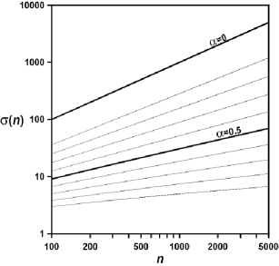
We then calculate the standard deviation $\sigma\left(n\right)$ using the original map. The results for $\alpha$ from $0$ to $0.9$ are shown in Fig. 1, where for large $n$ ($t>1000\,\tau$) the curves have no perceptible difference with $n^{1-\alpha}$.

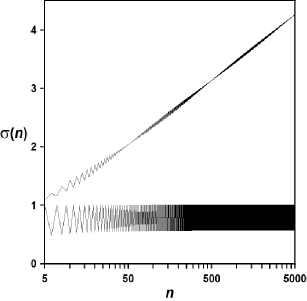
In Fig. 2 the upper curve, that corresponds to the standard deviation for $\alpha=1$, shows some quick oscillations governed by an average logarithmic evolution as was numerically checked for large times. The lower curve, for $\alpha=2$, shows that the standard deviation oscillates around a constant value. Then in both cases the average behavior agrees with the theoretical predictions.

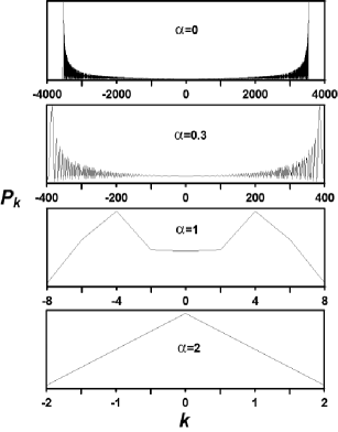
The profiles of the distribution $P_{k}$ for several values of $\alpha$ are shown in Fig. 3 at the same time $t=5000\,\tau$. For $\alpha=0$ the known QW profile for the Hadamard coin is obtained. In this case the function spreads with its greatest speed arriving up to the positions $\pm 3500$. For larger values of $\alpha$ the spreading speed decreases, the distribution shrinks and the two extreme peaks of the distribution come closer. When $\alpha=0.5$ the standard deviation spreads out as $\sigma(t)\sim t^{1/2}$, but the probability distribution $P_{k}$ is not Gaussian, it has the same characteristics as shown in Fig. 3 for $\alpha=0.3$. This confirms that the evolution corresponds to a coherent unitary process and not to the classical random walk. In the extreme case when $\alpha>1$ the distribution is restricted to small values around its initial value and the two extreme peaks have melt in a very narrow peak. We conclude that in all cases the asymptotic behaviors have an excellent agreement with the theoretical predictions.

IV Conclusion

In the usual QW the standard deviation has a linear growth, however using a biased quantum coin arranged in aperiodic sequence a sub-ballistic behavior is obtained Ribeiro . Here we generalize the discrete QW using a time dependent unitary coin operator. We find an analytical expression for the dependence of the standard deviation on the coin operator in the asymptotic regime. This expression shows explicitly how to select the unitary evolution to obtain a predetermined asymptotic behavior for the wave function spreading: ballistic, sub-ballistic, diffusive, sub-diffusive or localized. The parameter $\alpha$ of Eq.(19) determines the degree of diffusivity of the system for large times. This feature opens interesting possibilities for quantum information processing because it could be used for controlling the spreading of the wave function.

Finally another point worth mentioning is that the asymptotic differential Eq.(10) has the same form that the differential equation for the amplitudes of the quantum kicked rotor (QKR) in resonance Izrailev . The similitude between the QW and the QKR in resonance, suggested in Refs. alejo1 ; auyuanet ; alejo6 , has been recently extended to the anomalous diffusion behavior presented in this work NewQKR . Therefore, as the QKR has been realized experimentally Moore and the quantum resonances have already been observed Bharucha ; Kanem , our results for the QW could be experimentally confirmed through an implementation of the QKR in resonance.

We acknowledge the support from PEDECIBA, ANII and thank V. Micenmacher for his comments and stimulating discussions.

Appendix A

The first and second moments of the distribution $P_{k}$ are

$$m_{1}(t) = \sum_{k=-\infty}^{\infty}kP_{k}(t),$$ (22)

$$m_{2}(t) = \sum_{k=-\infty}^{\infty}k^{2}P_{k}(t).$$ (23)

Substituting Eq.(14) into these equations we have

$$m_{1}(t) = \sum_{j,l=\infty}^{\infty}\left(-1\right)^{-(j+l)}\left(a_{l}^{0}a_{j}^{0\ast}+b_{l}^{0}b_{j}^{0\ast}\right)F_{jl},$$ (24)

$$m_{2}(t) = \sum_{j,l=\infty}^{\infty}\left(-1\right)^{-(j+l)}\left(a_{l}^{0}a_{j}^{0\ast}+b_{l}^{0}b_{j}^{0\ast}\right){G}_{jl},$$ (25)

where

$$F_{jl} = \sum_{k=-\infty}^{\infty}k\text{ }J_{k-l}(t)J_{k-j}(t),$$ (26)

$$G_{jl} = \sum_{k=-\infty}^{\infty}k^{2}\text{ }J_{k-l}(t)J_{k-j}(t).$$ (27)

With the change of indexes $\mu=k-l$ and $\nu=l-j$, these equations become

$${F}_{jl} = \sum_{\mu=-\infty}^{\infty}\mu\text{ }J_{\mu}(t)J_{\mu-\nu}(t)$$ (28)

$$+l\sum_{\mu=-\infty}^{\infty}J_{\mu}(t)J_{\mu-\nu}(t),$$

$${G}_{jl} = \sum_{\mu=-\infty}^{\infty}\mu^{2}\text{ }J_{\mu}(t)J_{\mu-\nu}(t)$$ (29)

$$+2l\sum_{\mu=-\infty}^{\infty}\mu\text{ }J_{\mu}(t)J_{\mu-\nu}(t)$$

$$+l^{2}\sum_{\mu=-\infty}^{\infty}J_{\mu}(t)J_{\mu-\nu}(t).$$

In the above equations, three different type of sums are involved. They can be expressed in terms of the Kronecker delta using the propertied of the Bessel functions (Ref.Gradshteyn , p. 992, Eq. 8.530)

$$\sum_{\mu=-\infty}^{\infty}J_{\mu}(t)J_{\mu-\nu}(t) = \delta_{\nu 0},$$ (30)

$$\sum_{\mu=-\infty}^{\infty}\mu\text{ }J_{\mu}(t)J_{\mu-\nu}(t) = \frac{t}{2}\left(\delta_{\nu-1}+\delta_{\nu 1}\right),$$ (31)

$$\sum_{\mu=-\infty}^{\infty}\mu^{2}J_{\mu}(t)J_{\mu-\nu}(t) = \left(\frac{t}{2}\right)^{2}\left(\delta_{\nu-2}+2\delta_{\nu 0}+\delta_{\nu 2}\right)$$ (32)

$$+\frac{t}{2}\left(\delta_{\nu-1}-\delta_{\nu 1}\right).$$

Substituting the above equations into Eqs.(28, 29) and returning to the original indexes

$${F}_{jl} = l\text{ }\delta_{lj}+\frac{t}{2}\left(\delta_{lj-1}+\delta_{lj+1}\right),$$ (33)

$${G}_{jl} = \left(\frac{t}{2}\right)^{2}\delta_{lj-2}+\frac{t}{2}\left(2l+1\right)\delta_{lj-1}$$ (34)

$$+\left[2\left(\frac{t}{2}\right)^{2}+l^{2}\right]\delta_{lj}$$

$$+\frac{t}{2}\left(2l-1\right)\delta_{lj+1}+\left(\frac{t}{2}\right)^{2}\delta_{lj+2}.$$

Finally, Eqs.(15, 16) are obtained substituting Eqs.(33, 34) into Eqs.(24, 25).

References

- (1) J. Kempe, Contemp. Phys., 44, 307 (2003).
- (2) Y. Aharonov, L. Davidovich, and N. Zagury, Phys. Rev. A 48, 1687 (1993).
- (3) A.M. Childs, Phys. Rev. Lett. 102, 180501 (2009).
- (4) W. Dür, R. Raussendorf, V.M. Kendon, and H.J. Briegel, Phys. Rev. A 66, 052319, (2002).
- (5) B.C. Travaglione and G.J. Milburn, Phys. Rev. A 65, 032310, (2002).
- (6) B.C. Sanders, S.D. Bartlett, B. Tregenna, and P.L. Knight, Phys. Rev. A 67, 042305 (2003).
- (7) P.L. Knight, E. Roldán, and J.E. Sipe, Phys. Rev. A 68, 020301(R), (2003).
- (8) C. Cohen-Tannoudji, Rev. Mod. Phys. 70, 707 (1998).
- (9) J.I. Cirac and P. Zoller, Phys. Rev. Lett. 74, 4091 (1995).
- (10) B. Tregenna, W. Flanagan, R. Maile, and V. Kendon, New J. Phys. 5 83 (2003).
- (11) T. A. Brun, H. A. Carteret and A. Ambainis, Phys. Rev. A 67, 032304 (2003).
- (12) V. Kendon and B. Tregenna, Phys. Rev. A 67, 042315 (2003).
- (13) V. Kendon, Math. Struc. Comp. Sci. 17, 1169 (2007).
- (14) T. A. Brun, H. A. Carteret and A. Ambainis, Phys. Rev. A 67, 052317 (2003).
- (15) A. Wójcik, T. Luczak, P. Kurzynski, A. Grudka, and M. Bednarska, Phys. Rev. Lett. 93, 180601 (2004).
- (16) A. Romanelli, A. Auyuanet, R. Siri, G. Abal, and R. Donangelo. Physica A, 352, 409 (2005).
- (17) M. C. Bañuls, C. Navarrete, A. Pérez, E. Roldán, and J. C. Soriano, Phys. Rev. A 73, 062304 (2006).
- (18) C. Navarrete-Benlloch, A. Pérez, and E. Roldán, Phys. Rev. A 75, 062333 (2007).
- (19) P. Ribeiro, P. Milman, and R. Mosseri, Phys. Rev. Lett. 93, 190503 (2004).
- (20) A. Romanelli, Phys. Rev. A 76, 054306 (2007).
- (21) A. Romanelli, R. Siri, and V. Micenmacher, Phys. Rev. E 76, 037202 (2007).
- (22) N. Konno, Quant. Inf. Process. 1, 345 (2002).
- (23) F.M. Izrailev, Phys. Rep. 196, 299 (1990).
- (24) A. Romanelli, A.C. Sicardi Schifino, R. Siri, G. Abal, A. Auyuanet, and R. Donangelo. Physica A, 338, 395 (2004).
- (25) A. Romanelli, G. Hernández in quant-ph/0908.4596 (2009).
- (26) F.L. Moore, J.C. Robinson, C. Bharucha, P.E. Williams, M.G. Raizen, Phys. Rev. Lett. 73, 2974 (1994); J.C. Robinson, et al., ibid. 74, 3963 (1995); F.L. Moore, J.C. Robinson,C.F. Bharucha, B. Sundaram, M.G. Raizen, ibid. 75, 4598 (1995); J.C. Robinson,et al., ibid. 76, 3304 (1996).
- (27) C.F. Bharucha, J.C. Robinson, F.L. Moore, Bala Sundaram, Qian Niu, and M.G. Raizen, Phys. Rev. E 60, 3881 (1999).
- (28) J.F. Kanem, S. Maneshi, M. Partlow, M. Spanner and A. M. Steinberg, Phys. Rev. Lett. 98, 083004 (2007).
- (29) I.S. Gradshteyn, and I.M. Ryzhik, Table of Integrals Series and Products, (Academic Press, San Diego, 1994).