Harmonic oscillator in a one–dimensional box

Paolo Amore† and Francisco M Fernández 222Corresponding author † Facultad de Ciencias, Universidad de Colima, Bernal Díaz del Castillo 340, Colima, Colima, Mexico paolo@ucol.mx ‡ INIFTA (UNLP, CCT La Plata-CONICET), División Química Teórica, Blvd. 113 S/N, Sucursal 4, Casilla de Correo 16, 1900 La Plata, Argentina fernande@quimica.unlp.edu.ar
Abstract

We study a harmonic molecule confined to a one–dimensional box with impenetrable walls. We explicitly consider the symmetry of the problem for the cases of different and equal masses. We propose suitable variational functions and compare the approximate energies given by the variation method and perturbation theory with accurate numerical ones for a wide range of values of the box length. We analyze the limits of small and large box size.

1 Introduction

During the last decades there has been great interest in the model of a harmonic oscillator confined to boxes of different shapes and sizes[1, 2, 3, 4, 5, 6, 7, 8, 9, 10, 11, 12, 13, 14, 15, 16, 17, 18, 19, 20, 21, 22, 23]. Such model has been suitable for the study of several physical problems ranging from dynamical friction in star clusters[4] to magnetic properties of solids[6] and impurities in quantum dots[23].

One of the most widely studied model is given by a particle confined to a box with impenetrable walls at $-L/2$ and $L/2$ bound by a linear force that produces a parabolic potential–energy function $V(x)=k(x-x_{0})^{2}/2$, where $|x_{0}|<L/2$. When $x_{0}=0$ the problem is symmetric and the eigenfunctions are either even or odd; such symmetry is broken when $x_{0}\neq 0$. Although interesting in itself, this model is rather artificial because the cause of the force is not specified. It may, for example, arise from an infinitely heavy particle clamped at $x_{0}$. In such a case we think that it is more interesting to consider that the other particle also moves within the box.

The purpose of this paper is the discussion of the model of two particles confined to a one–dimensional box with impenetrable walls. For simplicity we assume that the force between them is linear. In Sec. 2 we introduce the model and discuss some of its general mathematical properties. In Sec. 3 we discuss the solutions of the Schrödinger equation for small box lengths by means of perturbation theory. In Sec. 4 we consider the regime of large boxes and propose suitable variational functions. In Sec. 5 we compare the approximate energies provided by perturbation theory and the variational method with accurate numerical ones. Finally, in Sec. 6 we summarize the main results and draw additional conclusions.

2 The Model

As mentioned above, we are interested in a system of two particles of masses $m_{1}$ and $m_{2}$ confined to a one–dimensional box with impenetrable walls located at $x=-L/2$ and $x=L/2$. If we assume a linear force between the particles then the Hamiltonian operator reads

$$\hat{H}=-\frac{\hbar^{2}}{2}\left(\frac{1}{m_{1}}\frac{\partial^{2}}{\partial x_{1}^{2}}+\frac{1}{m_{2}}\frac{\partial^{2}}{\partial x_{2}^{2}}\right)+\frac{k}{2}(x_{1}-x_{2})^{2}$$ (1)

and the boundary conditions are $\psi=0$ when $x_{i}=\pm L/2$. It is convenient to convert it to a dimensionless form by means of the variable transformation $q_{i}=x_{i}/L$ that leads to:

$$\hat{H}_{d}=\frac{m_{1}L^{2}}{\hbar^{2}}\hat{H}=-\frac{1}{2}\left(\frac{\partial^{2}}{\partial q_{1}^{2}}+\beta\frac{\partial^{2}}{\partial q_{2}^{2}}\right)+\frac{\lambda}{2}\left(q_{1}-q_{2}\right)^{2}$$ (2)

where $\beta=m_{1}/m_{2}$, $\lambda=km_{1}L^{4}/\hbar^{2}$ and the boundary conditions become $\psi=0$ if $q_{i}=\pm 1/2$. Without loss of generality we assume that $0<\beta\leq 1$.

The free problem ($-\infty<x_{i}<\infty$) is separable in terms of relative and center–of–mass variables

$\displaystyle x$ $\displaystyle=$ $\displaystyle x_{1}-x_{2}$
$\displaystyle X$ $\displaystyle=$ $\displaystyle\frac{1}{M}\left(m_{1}x_{1}+m_{2}x_{2}\right),\;M=m_{1}+m_{2}$ (3)

respectively, that lead to

$$\hat{H}=-\frac{\hbar^{2}}{2}\left(\frac{1}{M}\frac{\partial^{2}}{\partial X^{2}}+\frac{1}{m}\frac{\partial^{2}}{\partial x^{2}}\right)+V(x),\;m=\frac{m_{1}m_{2}}{M}.$$ (4)

In this case we can factor the eigenfunctions as

$\displaystyle\psi_{Kv}(x_{1},x_{2})$ $\displaystyle=$ $\displaystyle e^{iKX}\phi_{v}(x)$
$\displaystyle-\infty$ $\displaystyle<$ $\displaystyle K<\infty,\;v=0,1,\ldots$ (5)

where $\phi_{v}(x)$ are the well–known eigenfunctions of the harmonic oscillator and the eigenvalues read

$$E_{Kv}=\frac{\hbar^{2}K^{2}}{2M}+\hbar\sqrt{\frac{k}{m}}\left(v+\frac{1}{2}\right).$$ (6)

However, because of the boundary conditions, any eigenfunction is of the form $\psi(x_{1},x_{2})=(L^{2}/4-x_{1}^{2})(L^{2}/4-x_{2}^{2})\Phi(x_{1},x_{2})$, where $\Phi(x_{1},x_{2})$ does not vanish at the walls. We clearly appreciate that the separation just outlined is not possible in the confined model.

When $\beta<1$ the transformations that leave the Hamiltonian operator (including boundary conditions) invariant are: identity $\hat{E}:(q_{1},q_{2})\rightarrow(q_{1},q_{2})$ and inversion $\hat{\imath}:(q_{1},q_{2})\rightarrow(-q_{1},-q_{2})$. Therefore, the eigenfunctions of $\hat{H}_{d}$ are basis for the irreducible representations $A_{g}$ and $A_{u}$ of the point group $S_{2}$[24] (also called $C_{i}$ by other authors).

On the other hand, when $\beta=1$ (equal masses) the problem exhibits the highest possible symmetry. The transformations that leave the Hamiltonian operator (including boundary conditions) invariant are: identity $\hat{E}:(q_{1},q_{2})\rightarrow(q_{1},q_{2})$, rotation by $\pi$ $C_{2}:(q_{1},q_{2})\rightarrow(q_{2},q_{1})$, inversion $\hat{\imath}:(q_{1},q_{2})\rightarrow(-q_{1},-q_{2})$, and reflection in a plane perpendicular to the rotation axis $\sigma_{h}:(q_{1},q_{2})\rightarrow(-q_{2},-q_{1})$. In this case the states are basis functions for the irreducible representations $A_{g}$, $A_{u}$, $B_{g}$, and $B_{u}$ of the point group $C_{2h}$[24].

3 Small box

When $\lambda\ll 1$ we can apply perturbation theory choosing the unperturbed or reference Hamiltonian operator to be $\hat{H}_{d}^{0}=\hat{H}_{d}(\lambda=0)$. Its eigenfunctions and eigenvalues are given by

$\displaystyle\varphi_{n_{1},n_{2}}^{(0)}(q_{1},q_{2})$ $\displaystyle=$ $\displaystyle\left\{\begin{array}[]{ll}2\cos[(2i-1)\pi q_{1}]\cos[(2j-1)\pi q_{2}]&A_{g}\\ 2\sin(2i\pi q_{1})\sin(2j\pi q_{2})&A_{g}\\ 2\cos[(2i-1)\pi q_{1}]\sin(2j\pi q_{2})&A_{u}\\ 2\sin(2i\pi q_{1})\cos[(2j-1)\pi q_{2}]&A_{u}\end{array}\right.,\;i,j=1,2,\ldots$ (11)
$\displaystyle\epsilon_{n_{1},n_{2}}^{(0)}$ $\displaystyle=$ $\displaystyle\frac{\pi^{2}}{2}\left(n_{1}^{2}+\beta n_{2}^{2}\right),\;n_{1},\,n_{2}=1,2,\ldots.$ (12)

There is no degeneracy when $\beta<1$, except for the accidental one that takes place for particular values of $\beta$ which we will not discuss in this paper. The energies corrected to first order read

$$\epsilon_{n_{1},n_{2}}^{[1]}=\frac{\pi^{2}}{2}\left(n_{1}^{2}+\beta n_{2}^{2}\right)+\lambda\frac{\pi^{2}n_{1}^{2}n_{2}^{2}-3\left(n_{1}^{2}+n_{2}^{2}\right)}{12\pi^{2}n_{1}^{2}n_{2}^{2}}.$$ (13)

When $\beta=1$ the zeroth–order states $\varphi_{n_{1},n_{2}}^{(0)}$ and $\varphi_{n_{2},n_{1}}^{(0)}$ ($n_{1}\neq n_{2}$) are degenerate but it is not necessary to resort to perturbation theory for degenerate states in order to obtain the first–order energies. We simply take into account that the eigenfunctions of $\hat{H}_{d}^{0}$ adapted to the symmetry of the problem are

$$\varphi_{n_{1},n_{2}}^{(0)}(q_{1},q_{2})=\left\{\begin{array}[]{ll}\sqrt{2-\delta_{ij}}\left\{\cos[(2i-1)\pi q_{1}]\cos[(2j-1)\pi q_{2}]\right.&\\ \left.+\cos[(2j-1)\pi q_{1}]\cos[(2i-1)\pi q_{2}]\right\}&A_{g}\\ &\\ \sqrt{2}\left\{\cos[(2i-1)\pi q_{1}]\cos[(2j-1)\pi q_{2}]\right.&\\ \left.-\cos[(2j-1)\pi q_{1}]\cos[(2i-1)\pi q_{2}]\right\}&B_{g}\\ &\\ \sqrt{2}\left\{\cos[(2i-1)\pi q_{1}]\sin[2j\pi q_{2}]+\sin[2j\pi q_{1}]\cos[(2i-1)\pi q_{2}]\right\}&A_{u}\\ &\\ \sqrt{2}\left\{\cos[(2i-1)\pi q_{1}]\sin[2j\pi q_{2}]-\sin[2j\pi q_{1}]\cos[(2i-1)\pi q_{2}]\right\}&B_{u}\\ &\\ \sqrt{2-\delta_{ij}}\left\{\sin[2i\pi q_{1}]\sin[2j\pi q_{2}]+\sin[2j\pi q_{1}]\sin[2i\pi q_{2}]\right\}&A_{g}\\ &\\ \sqrt{2}\left\{\sin[2i\pi q_{1}]\sin[2j\pi q_{2}]-\sin[2j\pi q_{1}]\sin[2i\pi q_{2}]\right\}&B_{g}\end{array}\right.$$ (14)

where $i,j=1,2,\ldots$. They give us the energies corrected to first order as $\epsilon_{n}^{[1]}(S)=\left\langle\varphi_{ij}^{(0)}(S)\right|\hat{H}_{d}\left|\varphi_{ij}^{(0)}(S)\right\rangle$ where $S$ denotes the irreducible representation. Since some of these analytical expressions are rather cumbersome for arbitrary quantum numbers, we simply show the first sixth energy levels for future reference:

$\displaystyle\epsilon_{1}^{[1]}(A_{g})$ $\displaystyle=$ $\displaystyle\pi^{2}+\frac{\lambda(\pi^{2}-6)}{12\pi^{2}}$
$\displaystyle\epsilon_{1}^{[1]}(A_{u})$ $\displaystyle=$ $\displaystyle\frac{5\pi^{2}}{2}+\frac{\lambda(108\pi^{4}-405\pi^{2}-4096)}{1296\pi^{4}}$
$\displaystyle\epsilon_{1}^{[1]}(B_{u})$ $\displaystyle=$ $\displaystyle\frac{5\pi^{2}}{2}+\frac{\lambda(108\pi^{4}-405\pi^{2}+4096)}{1296\pi^{4}}$
$\displaystyle\epsilon_{2}^{[1]}(A_{g})$ $\displaystyle=$ $\displaystyle 4\pi^{2}+\frac{\lambda(2\pi^{2}-3)}{24\pi^{2}}$
$\displaystyle\epsilon_{3}^{[1]}(A_{g})$ $\displaystyle=$ $\displaystyle\epsilon_{1}^{[1]}(B_{g})=5\pi^{2}+\frac{\lambda(3\pi^{2}-10)}{36\pi^{2}}.$ (15)

The degeneracy of the approximate energies denoted $\epsilon_{3}^{[1]}(A_{g})$ and $\epsilon_{1}^{[1]}(B_{g})$ is broken at higher perturbation orders as shown by the numerical results in Sec. 5.

4 Large box

When $L\rightarrow\infty$ the energy eigenvalues tend to those of the free system (6). More precisely, we expect that the states with finite quantum numbers $n_{1}$, $n_{2}$ at $L=0$ correlate with those with $K=0$ when $L\rightarrow\infty$:

$$\lim_{\lambda\rightarrow\infty}\frac{\epsilon(\beta,\lambda)}{\sqrt{\lambda}}=\sqrt{1+\beta}\left(v+\frac{1}{2}\right),\;v=0,1,\ldots.$$ (16)

Besides, we should take into account that the symmetry of a given state is conserved as $L$ increases from 00 to $\infty$.

When $\beta<1$ we expect that the states approach

$$\psi_{Kv}(x,X)=\left\{\begin{array}[]{ll}\cos(KX)\phi_{2v}(x)&A_{g}\\ \sin(KX)\phi_{2v+1}(x)&A_{g}\\ \sin(KX)\phi_{2v}(x)&A_{u}\\ \cos(KX)\phi_{2v+1}(x)&A_{u}\end{array}\right.$$ (17)

as $L\rightarrow\infty$.

For the more symmetric case $\beta=1$ the states should be

$$\psi_{Kv}(x,X)=\left\{\begin{array}[]{ll}\cos(KX)\phi_{2v}(x)&A_{g}\\ \sin(KX)\phi_{2v}(x)&A_{u}\\ \cos(KX)\phi_{2v+1}(x)&B_{u}\\ \sin(KX)\phi_{2v+1}(x)&B_{g}\end{array}\right..$$ (18)

Obviously, the perturbation expressions (13) or (15) are unsuitable for this analysis and we have to resort to other approaches.

In order to obtain accurate eigenvalues and eigenfunctions for the present model we may resort to the Rayleigh–Ritz variational method and the basis set of eigenfunctions of $\hat{H}_{d}^{0}$ given in equations (12) and (14). Alternatively, we can also make use of the collocation method with the so–called little sinc functions (LSF) that proved useful for the treatment of coupled anharmonic oscillators[25]. In this paper we choose the latter approach.

Another way of obtaining approximate eigenvalues and eigenfunctions is provided by a straightforward variational method proposed some time ago[26]. The trial functions suitable for the present model are of the form

$$\varphi(q_{1},q_{2})=\left(\frac{1}{4}-q_{1}^{2}\right)\left(\frac{1}{4}-q_{2}^{2}\right)f(\mathbf{c},q_{1},q_{2})e^{-a(q_{1}-q_{2})^{2}}$$ (19)

where $\mathbf{c}=\{c_{1},c_{2},\ldots,c_{N}\}$ are linear variational parameters, which would give rise to the well known Rayleigh–Ritz secular equations, and $a$ is a nonlinear one. Even the simplest and crudest variational functions provide reasonable results for all values of $\lambda$ as shown in Sec. 5.

The simplest trial function for the ground state of the model with $\beta<1$ is

$$\varphi(q_{1},q_{2})=\left(\frac{1}{4}-q_{1}^{2}\right)\left(\frac{1}{4}-q_{2}^{2}\right)e^{-a(q_{1}-q_{2})^{2}}.$$ (20)

Notice that this function is basis for the irreducible representation $A_{g}$. We calculate $w(a,\lambda)=\left\langle\varphi\right|\hat{H}_{d}\left|\varphi\right\rangle/\left\langle\varphi\right.\left|\varphi\right\rangle$ and obtain $\lambda(a)$ from the variational condition $\partial w/\partial a=0$ so that $[w(a,\lambda(a)),\lambda(a)]$ is a suitable parametric representation of the approximate energy. In this way we avoid the tedious numerical calculation of $a$ for each given value of $\lambda$ and obtain an analytical parametric expression for the energy that we do not show here because it is rather cumbersome. We just mention that the parametric expression is valid for $a>a_{0}$ where $a_{0}$ is the greatest positive root of $\lambda(a)=0$.

When $\beta=1$ we choose the following trial functions for the lowest states of each symmetry type

$\displaystyle\varphi_{A_{g}}(q_{1},q_{2})$ $\displaystyle=$ $\displaystyle\left(\frac{1}{4}-q_{1}^{2}\right)\left(\frac{1}{4}-q_{2}^{2}\right)e^{-a(q_{1}-q_{2})^{2}}$
$\displaystyle\varphi_{A_{u}}(q_{1},q_{2})$ $\displaystyle=$ $\displaystyle\left(\frac{1}{4}-q_{1}^{2}\right)\left(\frac{1}{4}-q_{2}^{2}\right)(q_{1}+q_{2})e^{-a(q_{1}-q_{2})^{2}}$
$\displaystyle\varphi_{B_{u}}(q_{1},q_{2})$ $\displaystyle=$ $\displaystyle\left(\frac{1}{4}-q_{1}^{2}\right)\left(\frac{1}{4}-q_{2}^{2}\right)(q_{1}-q_{2})e^{-a(q_{1}-q_{2})^{2}}$
$\displaystyle\varphi_{B_{g}}(q_{1},q_{2})$ $\displaystyle=$ $\displaystyle\left(\frac{1}{4}-q_{1}^{2}\right)\left(\frac{1}{4}-q_{2}^{2}\right)\left(q_{1}^{2}-q_{2}^{2}\right)e^{-a(q_{1}-q_{2})^{2}}.$ (21)

5 Results

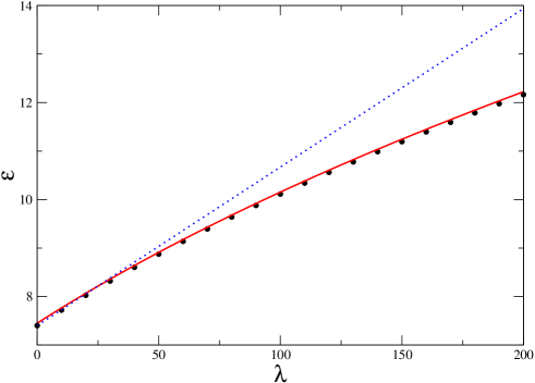
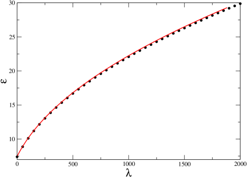
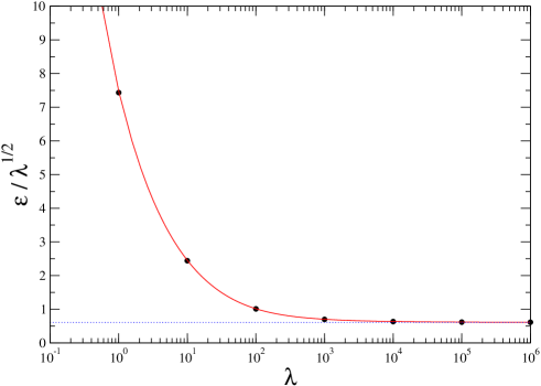
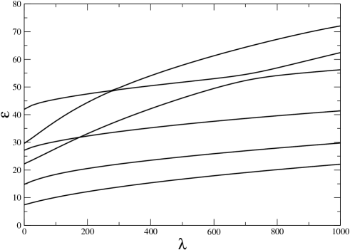
Fig. 1 shows the ground–state energy for $\beta=1/2$ calculated by means of perturbation theory, the LSF method and the variational function (20) for small and moderate values of $\lambda$. Fig. 2 shows the results of the latter two approaches for a wider range of values of $\lambda$. We appreciate the accuracy of the energy provided by the simple variational function (20) for all values of $\lambda$. The reader will find all the necessary details about the LSF collocation method elsewhere[25]. Here we just mention that a grid with $N=60$ was sufficient for the calculations carried out in this paper. Fig. 3 shows that $\epsilon(\lambda)/\sqrt{\lambda}$ calculated by the same two methods for $\beta=1/2$ approaches $\sqrt{3/8}$ as suggested by equation (16). Fig. 4 shows the first six eigenvalues $\epsilon(\lambda)$ for $\beta=1/2$ calculated by means of the LSF collocation method. The level order to the left of the crossings is $\epsilon_{1}(A_{g})<\epsilon_{1}(A_{u})<\epsilon_{2}(A_{u})<\epsilon_{2}(A_{g})<\epsilon_{3}(A_{g})<\epsilon_{3}(A_{u})$. Notice the crossings between states of different symmetry and the avoided crossing between the states $2A_{u}$ and $3A_{u}$.

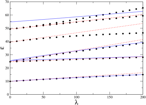
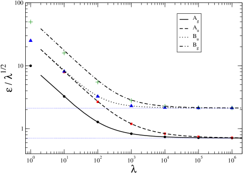
Fig. 5 shows the first six eigenvalues for $\beta=1$ calculated by means of perturbation theory, the LSF method and the variational functions (21) for small values of $\lambda$. The energy order is $\epsilon_{1}(A_{g})<\epsilon_{1}(A_{u})<\epsilon_{1}(B_{u})<\epsilon_{2}(A_{g})<\epsilon_{3}(A_{g})<\epsilon_{1}(B_{g})$ and we appreciate the splitting of the energy levels $\epsilon_{3}(A_{g})$ and $\epsilon_{1}(B_{g})$ that does not take place at first order of perturbation theory as discussed in Sec. 3. Finally, Fig. 6 shows $\epsilon(\lambda)/\sqrt{\lambda}$ for sufficiently large values of $\lambda$. We appreciate that the four simple variational functions (21) are remarkably accurate and that $\epsilon(\lambda)/\sqrt{\lambda}\rightarrow 1/\sqrt{2}$ for the first two states of symmetry $A_{g}$ and $A_{u}$ and $\epsilon(\lambda)/\sqrt{\lambda}\rightarrow 3/\sqrt{2}$ for the next two ones of symmetry $B_{u}$ and $B_{g}$. These results are consistent with equation (18) that suggests that the energies of the states with symmetry $A$ and $B$ approach $\sqrt{2}(2v+1/2)$ and $\sqrt{2}(2v+3/2)$, respectively. In fact, Fig. 6 shows four particular examples with $v=0$.

6 Conclusions

The model discussed in this paper is different from those considered before[1, 2, 3, 4, 5, 6, 7, 8, 9, 10, 11, 12, 13, 14, 15, 16, 17, 18, 19, 20, 21, 22, 23] because in the present case the linear force is due to the interaction between two particles. Although the interaction potential depends on the distance between the particles the problem is not separable and should be treated as a two–dimensional eigenvalue equation. It is almost separable for a sufficiently small box because the interaction potential is negligible in such limit and also for a sufficiently large box where the boundary conditions have no effect. It is convenient to take into account the symmetry of the problem and classify the states in terms of the irreducible representations because it facilitates the discussion of the connection between both regimes.

The model may be suitable to investigate the effect of pressure on the vibrational spectrum of a diatomic molecule and in principle one can calculate the spectral lines by means of the Rayleigh–Ritz or the LSF collocation method[25].

The simple variational functions developed some time ago [26] and adapted to present problem in Sec. 4 provide remarkably accurate energies for all values of the box size and are, for that reason, most useful to show the connection between both regimes and to verify the accuracy of more elaborate numerical calculations.

References

  • [1] Auluck F C and Kothari D S 1940 Science and Culture 7 370.
  • [2] Auluck F C 1941 Proc. Nat. Inst. India 7 133.
  • [3] Auluck F C 1942 Proc. Nat. Inst. India 8 147.
  • [4] Chandrasekhar S 1943 Astrophys. J. 97 263.
  • [5] Auluck F C and Kothari D S 1945 Proc. Camb. Phil. Soc. 41 175.
  • [6] Dingle R B 1952 Proc. Roy. Soc. London Ser. A 212 47.
  • [7] Baijal J S and Singh K K 1955 Prog. Theor. Phys. 14 214.
  • [8] Dean P 1966 Proc. Camb. Phil. Soc. 62 277.
  • [9] Vawter R 1968 Phys. Rev. 174 749.
  • [10] Vawter R 1973 J. Math. Phys. 14 1864.
  • [11] Consortini A and Frieden B R 1976 Nuovo Cim. B 35 153.
  • [12] Adams J E and Miller W H 1977 J. Chem. Phys. 67 5775.
  • [13] Rotbar F C 1978 J. Phys. A 11 2363.
  • [14] Aguilera-Navarro V C, Ley Koo E, and Zimerman A H 1980 J. Phys. A 13 3585.
  • [15] Aguilera-Navarro V C, Iwamoto H, Ley Koo E, and Zimerman A H 1981 Nuovo Cim. B 62 91.
  • [16] Barakat R and Rosner R 1981 Phys. Lett. A 83 149.
  • [17] Fernández F M and Castro E A 1981 Phys. Rev. A 24 2883.
  • [18] Fernández F M and Castro E A 1981 J. Math. Phys. 22 1669.
  • [19] Aguilera-Navarro V C, Gomes J F, Zimerman A H, and Ley Koo E 1983 J. Phys. A 16 2943.
  • [20] Chaudhuri R N and Mukherjee B 1983 J. Phys. A 16 3193.
  • [21] Mei W N and Lee Y C 1983 J. Phys. A 16 1623.
  • [22] Aquino N 1997 J. Phys. A 30 2403.
  • [23] Varshni Y P 1998 Superlattice Microst 23.
  • [24] Tinkham M 1964 Group Theory and Quantum Mechanics (McGraw-Hill, New York).
  • [25] Amore P and Fernández F M, Variational collocation for systems of coupled anharmonic oscillators, arXiv: 0905.1038v1 [quant-ph]
  • [26] Arteca G A, Fernández F M, and Castro E A 1984 J. Chem. Phys. 80 1569.
Refer to caption
Figure 1: Perturbation theory (dotted line), LSF (points) and variational (solid line) calculation of the ground–state energy $\epsilon(\lambda)$ for $\beta=1/2$.
Refer to caption
Figure 2: Variational (line) and LSF (points) calculation of the ground–state $\epsilon(\lambda)$ for $\beta=1/2$.
Refer to caption
Figure 3: Variational (line) and LSF (points) calculation of the ground–state $\epsilon(\lambda)/\sqrt{\lambda}$ for $\beta=1/2$. The horizontal line marks the limit $\sqrt{3/8}$.
Refer to caption
Figure 4: First six eigenvalues for $\beta=1/2$ calculated by means of the LSF method.
Refer to caption
Figure 5: First six eigenvalues for $\beta=1$. Circles, dotted line and solid line correspond to LSF collocation approach, perturbation theory and variation method, respectively. The level order is $A_{g}<A_{u}<B_{u}<2A_{g}<3A_{g}<B_{g}$.
Refer to caption
Figure 6: Variational (solid line) and LSF (symbols) calculation of $\epsilon(\lambda)/\sqrt{\lambda}$ for $\beta=1$. The horizontal lines mark the limits $1/\sqrt{2}$ and $3/\sqrt{2}$.