Likelihood Functions for Supersymmetric Observables in Frequentist Analyses of the CMSSM and NUHM1
Abstract
On the basis of frequentist analyses of experimental constraints from electroweak precision data, , physics and cosmological data, we investigate the parameters of the constrained MSSM (CMSSM) with universal soft supersymmetry-breaking mass parameters, and a model with common non-universal Higgs masses (NUHM1). We present likelihood functions for the masses of supersymmetric particles and Higgs bosons, as well as BR(), BR() and the spin-independent dark matter scattering cross section, . In the CMSSM we find preferences for sparticle masses that are relatively light. In the NUHM1 the best-fit values for many sparticle masses are even slightly smaller, but with greater uncertainties. The likelihood functions for most sparticle masses are cut off sharply at small masses, in particular by the LEP Higgs mass constraint. Both in the CMSSM and the NUHM1, the coannihilation region is favoured over the focus-point region at about the 3- level, largely but not exclusively because of . Many sparticle masses are highly correlated in both the CMSSM and NUHM1, and most of the regions preferred at the 95% C.L. are accessible to early LHC running, though high-luminosity running would be needed to cover the regions allowed at the 3- levels. Some slepton and chargino/neutralino masses should be in reach at the ILC. The masses of the heavier Higgs bosons should be accessible at the LHC and the ILC in portions of the preferred regions in the plane. In the CMSSM, the likelihood function for BR() is peaked close to the Standard Model value, but much larger values are possible in the NUHM1. We find that values of pb are preferred in both the CMSSM and the NUHM1. We study the effects of dropping the , BR(), and constraints, demonstrating that they are not in tension with the other constraints.
CERN-PH-TH/2009-124, DCPT/09/112, FTPI-MINN-09/24, IPPP/09/56, UMN-TH-2804/09
1 Introduction
Supersymmetry (SUSY) [1, 2, 3] is one of the favoured ideas for physics beyond the Standard Model (SM) that may soon be explored at the Large Hadron Collider (LHC). In a recent paper [4], we presented some results from frequentist analyses of the parameter spaces of the constrained minimal supersymmetric extension of the Standard Model (CMSSM) — in which the soft supersymmetry-breaking scalar and gaugino masses are each constrained to universal values and , respectively [5, 6, 7, 8, 9, 10, 11, 12, 13, 14, 15, 16, 17, 18, 19, 20, 21, 22, 23, 24] — and the NUHM1 — in which the soft supersymmetry-breaking contributions to the Higgs masses are allowed a different but common value [25, 26, 27]. Other statistical analyses in these models can be found in [28, 29, 30, 31, 32, 33, 34, 35, 36, 37, 38, 39] and Markov Chain Monte Carlo (MCMC) analyses in [40, 41, 42, 43, 44, 45, 46, 47, 48, 49, 50, 51, 52, 53, 54, 55, 56, 57]. For comparison, see also [58, 59] for recent analyses in the next-to-minimal extension of the SM, as well as [60, 61, 62] for other analyses in supersymmetric models without a dedicated fit.
The results presented in [4] included the parameters of the best-fit points in the CMSSM and the NUHM1, as well as the 68 and 95% C.L. regions found with default implementations of the phenomenological, experimental and cosmological constraints. These include precision electroweak data, the anomalous magnetic moment of the muon, , -physics observables (the rates for BR() and BR(), mixing, and the upper limit on BR()), the bound on the lightest MSSM Higgs boson mass, , and the cold dark matter (CDM) density inferred from astrophysical and cosmological data 111We did not include the constraint imposed by the experimental upper limit on the spin-independent DM scattering cross section , which is subject to astrophysical and hadronic uncertainties, as discussed below., assuming that this is dominated by the relic density of the lightest neutralino, . We also discussed in [4] the sensitivities of the areas of the preferred regions to changes in the ways in which the major constraints are implemented. We found that the smallest sensitivity was to the CDM density, and the greatest sensitivity was that to .
In this paper we adopt the frequentist approach from [4], which is different from the Bayesian approach adopted in [41, 42, 43, 44, 45, 46, 47, 48, 49, 50, 51, 52]. A key issue in a Bayesian approach is the appropriate choice of priors. As discussed in some recent Bayesian analyses of the CMSSM [45, 46, 52], conclusions for preferred regions of parameter space can depend the choice of priors. In our view, the results of a Bayesian approach should not be considered definitive unless they are shown to be sufficiently independent of plausible variations in the choice of priors. In our frequentist analysis, we use the MCMC technique to sample efficiently the CMSSM and NUHM1 parameter spaces, and we generate sufficiently many chains to sample adequately these parameter spaces, as discussed in more detail in Section 2 of this paper.
Our treatments of the experimental constraints from electroweak precision observables, -physics observables and cosmological data are, in general, very similar to those in [4]. Accordingly, we do not discuss details in this paper, contenting ourselves with a brief recapitulation and update.
In Section 3 we extend the presentation of results from our MCMC frequentist analysis to include the global likelihood functions for various observables, including , BR(), BR() and the spin-independent DM scattering cross section, , as well as sparticle masses. We also discuss the correlations between pairs of these observables, and compare the results in the CMSSM and NUHM1. We pay particular attention to the prospects for detecting SUSY in forthcoming experiments, including searches at the LHC and the ILC as well as physics and direct searches for CDM.
We present an update on the prediction of in the CMSSM [53] and the first prediction for in the NUHM1. For these analyses the experimental constraints on itself have been left out of the fit. The result in the CMSSM of [53] is confirmed with a best-fit value slightly below the LEP bound. Within the NUHM1, however, a value above the LEP bounds arises naturally. For other observables, however, the information is included in calculating the likelihood functions. The likelihood functions for generic sparticle masses are skewed, being cut off at low masses by the LEP lower limit on , in particular. On the other hand the likelihood functions rise more gradually for large masses, with the largest contribution arising from . We see that the role of the constraint is smaller in the NUHM1 than in the CMSSM, reflecting the fact that the other constraints suggest, in the NUHM1, a value of somewhat larger than the LEP lower limit.
As remarked in [4], the preferred values of the sparticle masses are generally somewhat lower in the NUHM1 than in the CMSSM. This is because the extra degree of freedom in the Higgs sector allows lower values of to be reconciled with upper limits on deviations from the SM and the LEP lower limit on . Recall that in the CMSSM, the Higgs mass mixing parameter, , and the Higgs pseudoscalar mass, , are fixed by the minimization of the Higgs potential ensuring electroweak symmetry breaking when is chosen as an input parameter. In contrast, in the NUHM1, either or can be chosen as an additional input parameter 222The choice of either or as an input is equivalent to a choice of the soft Higgs mass at the GUT scale., thus allowing substantial additional freedom in the light Higgs scalar mass for a given set of CMSSM parameters (). The greater freedom in the Higgs sector also results in different mass ranges being favoured for the heavier Higgs bosons and for the heavier neutralinos, as observed in [4].
We find here that sparticle masses are mostly highly correlated. This could be expected for and , which are both determined essentially uniquely by . However, the correlation is only slightly weakened for the slepton and squark masses, including . This is partly because the largest contributions to the preferred values of most of these particles are due to , rather than to . This tendency is reinforced by the fact that our likelihood analysis finds that the coannihilation regions are favoured in both the CMSSM and the NUHM1. However, this preference is slightly weakened in the NUHM1, where direct-channel annihilation through the heavy Higgs () poles may also play a subsidiary role, and larger values of become possible. In particular, the correlation between and is particularly weak in the NUHM1, reflecting the appearance of preferred regions of the parameters away from the coannihilation strip. In general, there are good prospects for discovering SUSY in early LHC running, in both the CMSSM and the NUHM1.
We find that BR() is expected to be close to its SM value in the CMSSM, because of the strong preference for relatively low where the supersymmetric contributions to this channel are small. They may be much larger in the NUHM1 because of the freedom to choose below its nominal CMSSM value. Spin-independent scattering of supersymmetric dark matter may well be observable in planned experiments in both the CMSSM and the NUHM1, where a somewhat larger range for is preferred in the NUHM1 [26, 63].
However, these optimistic conclusions rely critically on the implementation of the constraint using low-energy data, as used in our analysis, and we discuss in Section 6.1 the implications of removing the constraint. We also discuss the predictions of our fits for BR(), and , presenting the likelihood functions for each of these observables without their own contributions. None of these observables exhibits any significant tension with the others.
2 Description of the Frequentist Statistical Method Employed
We define a global likelihood function, which combines all theoretical predictions with experimental constraints:
| (1) |
Here is the number of observables studied, represents an experimentally measured value (constraint) and each defines a prediction for the corresponding constraint that depends on the supersymmetric parameters. The experimental uncertainty, , of each measurement is taken to be both statistically and systematically independent of the corresponding theoretical uncertainty, , in its prediction. We denote by and the contributions from the two measurements for which only one-sided bounds are available so far, as discussed below. Furthermore we include the lower limits from the direct searches for SUSY particles at LEP [64] as one-sided limits, denoted by “” in eq. (1).
We stress that, as in [4, 53], the three standard model parameters are included as fit parameters and allowed to vary with their current experimental resolutions . We do not include as a fit parameter, which would have only a minor impact on the analysis.
Formulating the fit in this fashion has the advantage that the probability, , properly accounts for the number of degrees of freedom, , in the fit and thus represents a quantitative and meaningful measure for the “goodness-of-fit.” In previous studies [53], has been verified to have a flat distribution, thus yielding a reliable estimate of the confidence level for any particular point in parameter space. Further, an important aspect of the formulation is that all model parameters are varied simultaneously in the MCMC sampling, and care is exercised to fully explore the multi-dimensional space, including possible interdependencies between parameters. All confidence levels for selected model parameters are performed by scanning over the desired parameters while minimizing the function with respect to all other model parameters. That is, in order to determine the function for some model parameter , all the remaining free parameters are set to values corresponding to a new minimum determined for fixed . The function values where is found to be equal to determine the confidence level contour. For two-dimensional parameter scans we use to determine the 68%(95%) confidence level contours.
Only experimental constraints are imposed when deriving confidence level contours, without any arbitrary or direct constraints placed on model parameters themselves.333For reasons of stability of higher-order contributions, we limit the range of to values below . As explained in Section 3 below, we furthermore impose a cut on parameter regions where the higher-order corrections relating the running mass to the on-shell mass of the pseudo-scalar Higgs boson get unacceptably large. This leads to robust and statistically meaningful estimates of the total 68% and 95% confidence levels, which may be composed of multiple separated contours. Finally, the sensitivity of the global fit to different constraint scenarios can be studied by removing one of the experimental constraints or by rescaling one of the experimental uncertainties, as discussed in Sect. 3 in [4]. Studies of such scenarios are particularly helpful in identifying which experimental data are most useful in constraining the theoretical model and hence in precisely studying how hyper-volumes in parameter space become more tightly constrained (either now or in the future).
Since each new scenario in which a parameter is removed or an uncertainty re-scaled represents, fundamentally, a new function which must be minimized, multiple re-samplings of the full multi-dimensional parameter space are, in principle, required to determine the most probable fit regions for each scenario. However, these would be computationally too expensive. To avoid this difficulty, we exploit the fact that independent functions are additive and result in a well defined probability. Hence, we define “loose” functions, , in which the term representing some constraint, e.g., , is removed from the global function. The function represents the likelihood that a particular set of model parameter values is compatible with a sub-set of the experimental data constraints, without any experimental knowledge of the removed constraint.
An exhaustive, and computationally expensive, 25 million point pre-sampling of the function is then performed in the full multi-dimensional model parameter space using a MCMC. Constraint terms representing the various experimental scenarios are then re-instated or removed to form different functions, one for each scenario studied. If the scenario requires an additional constraint to be removed from the function, the density of points pre-sampled for the function was carefully tested and verified to also be an unbiased and sufficiently complete sampling of the studied model parameter space for the full function by using dedicated MCMC samples of approximately one million sampling points each, where the particular constraint in question was removed. Specifically, we use this technique to study the effects of removing individually the , BR(), and constraints. The precise values of the most probable fit parameters are determined via a full MINUIT minimization of the for each different scenario, but are performed only within the general parameter space regions not already excluded from the pre-sampling of the function. An MCMC final sampling is subsequently used to determine the 68% and 95% confidence-level contours for each constraint scenario studied 444We note that for parameter space regions having low probability density, statistical fluctuations can appear in the form of an “archipelago of islands” near the 95% confidence levels. Such statistical fluctuations simply reflect the lower MCMC sampling density in regions of low probability..
For example, in [4] we showed that the effect of dropping the experimental data from the fit is not very important in constraining the allowed regions in the and planes. The reason for this can be understood by recalling that the WMAP strips in the CMSSM planes found for different, but fixed, values of move around as this and other CMSSM parameters are varied. Indeed, for fixed , the strips can be shown to nearly foliate the plane [19, 65]. Since is only weakly constrained by the experimental data but gets correlated through the fit to the other parameters (, , ), the effect of the constraint is to reduce the dimensionality of the allowed parameter-space to a certain “hyper-sheet” which, when viewed by fixing to a particular value (i.e. slicing the sheet along the -axis), reduces to the observed strips in the planes. However, since this sheet is generally embedded in the full parameter space hyper-volume and is not diagonalized along some particular parameter axis, a large range of values for remain statistically probable when considering the global fit and, from a strict statistical consideration, there are no strips of preferred regions.
When we apply here a similar analysis to the constraint, we find a very different picture. We exhibited already in [4] the effect of relaxing this constraint by some fraction, showing that the preferred areas of the and planes changed substantially. Here we illustrate the effect of removing the constraint entirely, which relaxes very considerably the upper limits on sparticle masses. However, the other observables still disfavour very large values of and by , as we discuss below.
3 Summaries of the CMSSM and NUHM1 Analyses
The experimental constraints used in our analyses are listed in Table 1. The notations for the observables are standard, and were defined in [53, 4]. Their values generally have only minor updates from the values quoted there, but one important comment concerns our implementation of the LEP constraint on . The value quoted in the Table was derived within the SM, and is applicable to the CMSSM, in which the relevant Higgs couplings are very similar to those in the SM [66, 67], so that the SM exclusion results can be used, supplemented with an additional theoretical uncertainty whose implementation we now describe.
| Observable | Th. Source | Ex. Source | Constraint | Add. Th. Unc. |
| [GeV] | [68, 69] | [70] | – | |
| [68, 69] | [71] | – | ||
| [GeV] | [68, 69] | [71] | – | |
| [GeV] | [68, 69] | [71] | 0.001 | |
| [nb] | [68, 69] | [71] | – | |
| [68, 69] | [71] | – | ||
| [68, 69] | [71] | – | ||
| [68, 69] | [71] | 0.1465 0.0032 | – | |
| [68, 69] | [71] | 0.21629 0.00066 | – | |
| [68, 69] | [71] | 0.1721 0.003 | – | |
| [68, 69] | [71] | 0.0992 0.0016 | – | |
| [68, 69] | [71] | 0.0707 0.0035 | – | |
| [68, 69] | [71] | 0.923 0.020 | – | |
| [68, 69] | [71] | 0.670 0.027 | – | |
| [68, 69] | [71] | 0.1513 0.0021 | – | |
| [68, 69] | [71] | 0.2324 0.0012 | – | |
| [GeV] | [68, 69] | [72, 73] | 0.010 | |
| BR | [74, 75, 76, 77, 78] | [79] | 0.050 | |
| BR | [80, 81, 82, 83] | [79] | ||
| BR | [82, 83, 84] | [85, 86, 87] | – | |
| [80, 81, 82, 83] | [79] | |||
| [88] | [79, 89] | – | ||
| BR | [82, 84] | [90] | – | |
| BR | [91] | [92] | – | |
| [91] | [93, 94] | – | ||
| [80, 81, 82, 83] | [79, 93, 94] | – | ||
| [91] | [93, 94] | – | ||
| [95, 96, 97, 98] | [99, 100, 101] | |||
| [GeV] | [102, 103, 104, 105] | [106, 107] | (see text) | 1.5 |
| [108, 109, 110] | [111] | 0.012 |
We evaluate the contribution within the CMSSM using the formula
| (2) |
with for 555We use so as to incorporate a conservative consideration of experimental systematic effects.. Larger masses do not receive a contribution. The in the denominator corresponds to a convolution of the likelihood function with a Gaussian function, , normalized to unity and centered around , whose width is , representing the theory uncertainty on [102]. In this way, a theoretical uncertainty of up to is assigned for of all values corresponding to one CMSSM parameter point. The term in the denominator corresponds to a parametrization of the curve given in the final SM LEP Higgs result [106].
Within the NUHM1 the situation is somewhat more involved, since, for instance, a strong suppression of the coupling can occur, invalidating the SM exclusion bounds. In order to find a more reliable 95% C.L. exclusion limit for in the case that the SM limit cannot be applied, we use the following procedure. The main exclusion bound from LEP searches comes from the channel . The Higgs boson mass limit in this channel is given as a function of the coupling in [107]. A reduction in the coupling in the NUHM1 relative to its SM value can be translated into a lower limit on the lightest NUHM1 Higgs mass, , shifted to lower values with respect to the SM limit of . (The actual number is obtained using the code HiggsBounds [112] that incorporates the LEP (and Tevatron) limits on neutral Higgs boson searches.) For values of the reduction of the couplings required to evade the LEP bounds becomes very strong, and we add a brick-wall contribution to the function below this value (which has no influence on our results). Finally, eq. (2) is used with to ensure a smooth transition to the SM case, where we use to allow for experimental systematics, as discussed above. This is a conservative approach in the sense that the term used in eq. (2) can be regarded as a lower limit on the spread of the curve in the vicinity of .
The numerical evaluation of the frequentist likelihood function using these constraints has been performed with the MasterCode [53, 4], which includes the following theoretical codes. For the RGE running of the soft SUSY-breaking parameters, it uses SoftSUSY [113], which is combined consistently with the codes used for the various low-energy observables. At the electroweak scale we have included various codes: FeynHiggs [102, 103, 104, 105] is used for the evaluation of the Higgs masses and (optionally) (see also [95, 96, 97, 98])666We recall that the experimental value appears to differ by over three standard deviations from the best SM calculation based on low-energy data [95, 99, 100, 114, 115, 116, 117], but that the discrepancy is significantly reduced if decay data are used to evaluate the SM prediction. We note that recently a new based analysis has appeared [118], which yields a deviation from the SM prediction. A new SM prediction based on radiative-return data from BABAR is in the offing.. For flavour-related observables we use SuFla [82, 83] as well as SuperIso [119, 120], and for the electroweak precision data we have included a code based on [68, 69]. Finally, for dark-matter-related observables, MicrOMEGAs [108, 109, 110] and DarkSUSY [121, 122] have been used. We made extensive use of the SUSY Les Houches Accord [123, 124] in the combination of the various codes within the MasterCode.
It is well known from previous comparisons that different RGE codes for the running of the soft SUSY-breaking parameters give quite different results in parameter regions where higher-order corrections get very large [125]. This happens in general for very large values of , but instabilities can also occur in, e.g., the evaluation of in the CMSSM. In such a case the evaluation of the impacts of constraints that are affected by the heavy Higgs bosons can become unreliable. Motivated by these observations, we made two cuts on the pre-sampled CMSSM and NUHM1 points in deriving the results presented below: we do not consider points with , and we have discarded parameter points where the difference between the running () mass of the pseudoscalar Higgs, , and the physical (on-shell) mass, , gets unacceptably large. For the latter, we have applied the condition . Imposing these cuts has no effect on the best-fit point, nor on the 68% C.L. range of any parameter of the fit 777However, discarding these points does reduce the 95% C.L. upper limit on in the NUHM1 by about 10%, from to . This difference may be regarded as a theoretical systematic uncertainty in the results.. Motivated by and (to a lesser extent) BR(), we restrict our study to .
For the parameters of the best-fit CMSSM point we find , , , and , yielding the overall (36% probability) and nominally 888This is acceptable, taking into account the theoretical uncertainty in the FeynHiggs calculation of [102], see the discussion above.. These values are very close to the ones reported in [4]. The corresponding parameters of the best-fit NUHM1 point are , , , and or, equivalently, , yielding (corresponding to a similar fit probability to the CMSSM) and . The similarity between the best-fit values of , and in the CMSSM and the NUHM1 suggest that the model frameworks used are reasonably stable: if they had been very different, one might well have wondered what would be the effect of introducing additional parameters, as in the NUHM2 [126, 127] with two non-universality parameters in the Higgs sector999Computationally, exploring adequately the NUHM2 parameter space using the frequentist approach would be very expensive, but we hope to return to it in the future..
These best-fit points are both in the coannihilation region of the plane, as can be seen in Fig. 1, which displays contours of the function in the CMSSM (left) and the NUHM1 (right). The C.L. contours extend to slightly larger values of in the CMSSM, while they extend to slightly larger values of in the NUHM1, as was already shown in [4] for the 68% and 95% C.L. contours. However, the qualitative features of the contours are quite similar in the two models, indicating that the preference for small and are quite stable and do not depend on details of the Higgs sector. We recall that it was found in [4] that the focus-point region was disfavoured at beyond the 95% C.L. in both the CMSSM and the NUHM1. We see in Fig. 1 that this region is disfavoured at the level in the CMSSM and in the NUHM1.

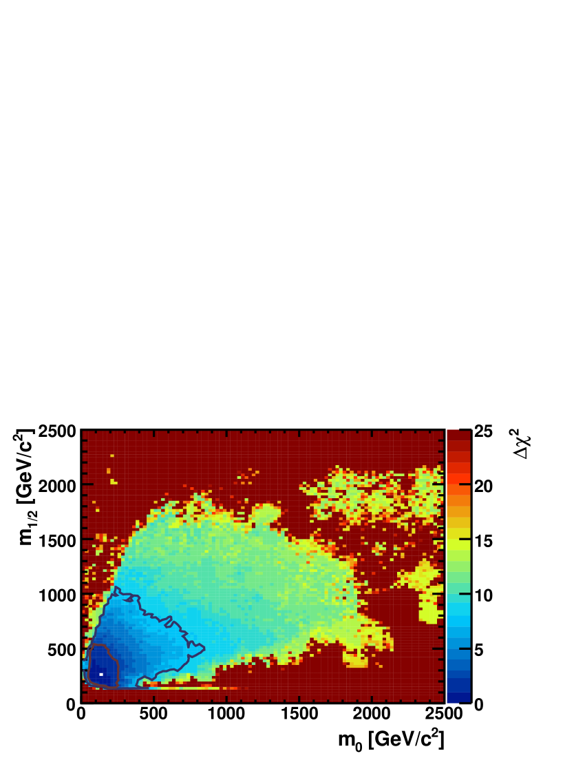
This feature is seen explicitly in the left and right panels of Fig 2, which display the likelihood functions for in the CMSSM and NUHM1, respectively. (We recall that the focus-point region would be found at .) Looking first at the solid lines corresponding to the full global fit, we also see explicitly that low values of are favoured in both cases, reflecting the fact that coannihilation points are generally favoured. The favoured regions also have relatively low values of , as seen in Fig. 1. As we discuss in more detail later, the minimum in both cases is found at low .
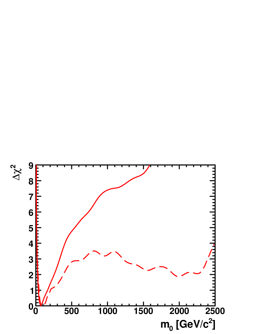
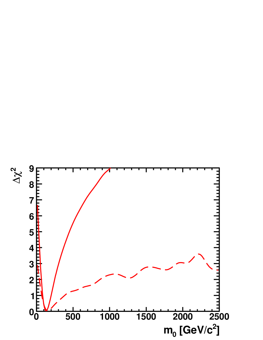
The large values of in the focus-point region are largely, but not entirely, due to the constraint, as can be seen in the dashed lines in Fig. 2, where this constraint has been removed. In the CMSSM case without , the global minimum at is followed by a local maximum around with . This is in turn followed by a secondary local minimum around with . The absolute minimum occurs in the coannihilation region, and the secondary minimum occurs in the focus-point region. The local maximum at intermediate reflects the fact that such values of are compatible with the dark matter constraint only at relatively large values of and that are disfavoured by other constraints. This is not the case in the NUHM1, where intermediate values of with relatively low values of are compatible with the constraint (thanks to the possible appearance of direct-channel Higgs poles), as well as the other constraints. See Section 6 below for a more detailed discussion of the impact of dropping the constraint.
We summarize in Table 2 the contributions to the global likelihood function at the best-fit points in the CMSSM and NUHM1 due to the most important observables as well as their total . We also list the contributions to for the best fit we find in the focus-point (FP) region for the CMSSM (considered to be that with ). This point has , , and . It is apparent from Table 2 that the focus-point region is disfavoured by , but also by , and that the contributions of the other observables fail to overcome this disadvantage. Indeed, many of the other observables favour independently the coannihilation region, e.g., BR(), 101010We note, however, that within the SM there is significant tension between the experimental value of and (LEP), and that this tension is not reduced significantly in the CMSSM or NUHM1, see also [69]. and — though the difference here is relatively small. Only and BR() and (b)(LEP) favour the FP region, but not with high significance.
| Observable | Best CMSSM fit | Best NUHM1 fit | Best CMSSM FP fit |
|---|---|---|---|
| 0.44 | 0.002 | 8.4 | |
| BR() | 0.20 | 0.41 | 0.85 |
| 0.53 | 0.08 | 1.5 | |
| 2.84 | 3.22 | 3.56 | |
| (LEP) | 7.61 | 7.08 | 6.74 |
| 0.96 | 1.01 | 1.05 | |
| 1.16 | 0.001 | 0.95 | |
| 0.17 | 0 | 0 | |
| 20.6 | 18.5 | 29.8 |
4 Likelihood Distributions for Sparticle Masses and Other Observables
In our previous paper [4] we discussed, in addition to the spectra at the best-fit points in the CMSSM and NUHM1, the regions of the planes preferred in these scenarios at the 68 and 95% C.L. Here we complement those discussions by providing directly the likelihood functions for certain sparticle masses, noting in particular the impacts of the most relevant constraints111111In each case, we show , the difference between the total function and its value at the minimum for the relevant model..
We start by discussing the likelihood functions for the mass of the neutralino LSP, , in the CMSSM and NUHM1. The left panel of Fig. 3 displays the likelihood function in the CMSSM. The solid line shows the result obtained when incorporating the LEP Higgs limit, while the dashed line corresponds to the case where the LEP Higgs constraint is removed. There is a sharp rise in the likelihood function at low values of , which is caused by the limits from the direct searches for SUSY particles, but receives also contributions from BR() and other constraints. This sharp rise in the likelihood function persists when the LEP Higgs constraint is removed, but is shifted towards slightly lower values of in that case. The right panel of Fig. 3 shows the likelihood function for in the NUHM1, again with and without the LEP constraint imposed. Including the LEP constraint we see that the optimal value of is somewhat smaller than in the CMSSM case, reflecting the lower value of at the corresponding best-fit point discussed in [4] 121212We recall that, to a very good approximation, in most of the relevant regions of the CMSSM and NUHM1 parameter spaces discussed here.. Finally, the dashed line in the right panel of Fig. 3 displays the likelihood function in the NUHM1 with the LEP Higgs constraint removed. Here we see very little difference from the result for the NUHM1 with the LEP constraint imposed. This reflects the fact that in the NUHM1 (unlike the CMSSM) the other constraints do not push down to quite low values, a point made explicit in Fig. 4 below.
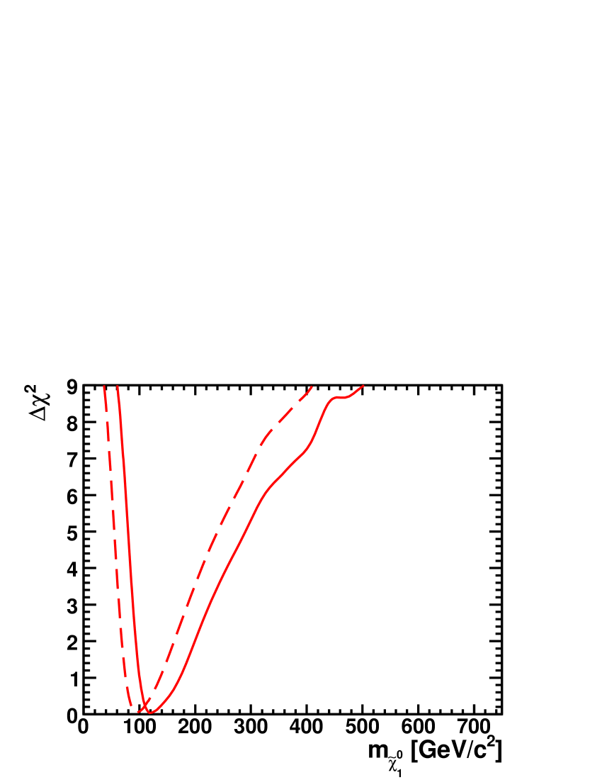
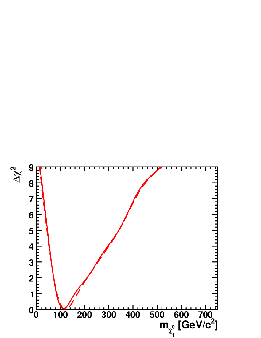
The gradual rises in the likelihood functions at large in both the CMSSM and the NUHM1 are dominated by the contribution of , discussed already above, which disfavours large (and ). We comment later on the impacts on and other observables if the constraint is removed.
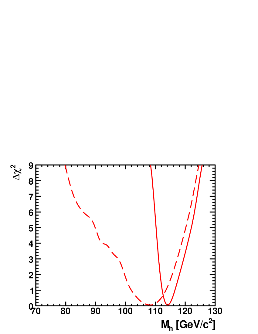
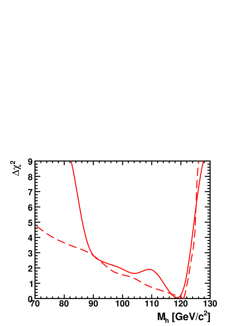
In order to see explicitly the importance of the constraint, we display in Fig. 4 the likelihood functions for in the CMSSM (left) and the NUHM1 (right), both with (solid lines) and without (dashed lines) the LEP constraint on . Comparing first the two CMSSM results, we see that the other constraints would prefer a value of somewhat below the SM Higgs limit from LEP [106] (this was already observed in [53]). The best fit value for is still acceptable in that case, in particular in view of the theoretical uncertainties in the CMSSM evaluation of , see the discussion above. However, in the case of the NUHM1, shown in the right plot of Fig. 4, the best-fit value of indicated by the other constraints is significantly higher than the SM LEP lower limit. As a consequence, incorporating the LEP constraint (see above for details), shown as the solid line, does not alter significantly the best-fit value of . As a corollary, the differences between the likelihood functions of the NUHM1 for other masses and observables between the fits with and without the LEP constraint are less significant than for the CMSSM. In the rest of this paper (except in Section 6.4) we show results with the LEP constraint imposed.
We discuss next the likelihood functions for various sparticle masses, which are summarized in Fig. 5. The results for the CMSSM spectrum are shown in the left plot, and for the NUHM1 in the right plot. We start our discussion with the gluino mass, . In both the CMSSM and the NUHM1, the best-fit points have relatively low values of and , respectively. These favoured values are well within the range even of the early operations of the LHC with reduced centre-of-mass energy and limited luminosity. However, the effect of the gradual increase in as increases, due essentially to as commented before, means that even quite large values of are allowed at the 3- () level (not shown in Fig. 5). The LHC should be able to discover a gluino with with 100/fb of integrated luminosity at [128, 129], and the proposed SLHC luminosity upgrade to 1000/fb of integrated luminosity at should permit the discovery of a gluino with [130]. However, Fig. 5 does demonstrate that, whilst there are good prospects for discovering SUSY in early LHC running [4], this cannot be ‘guaranteed’, even if one accepts the constraint.
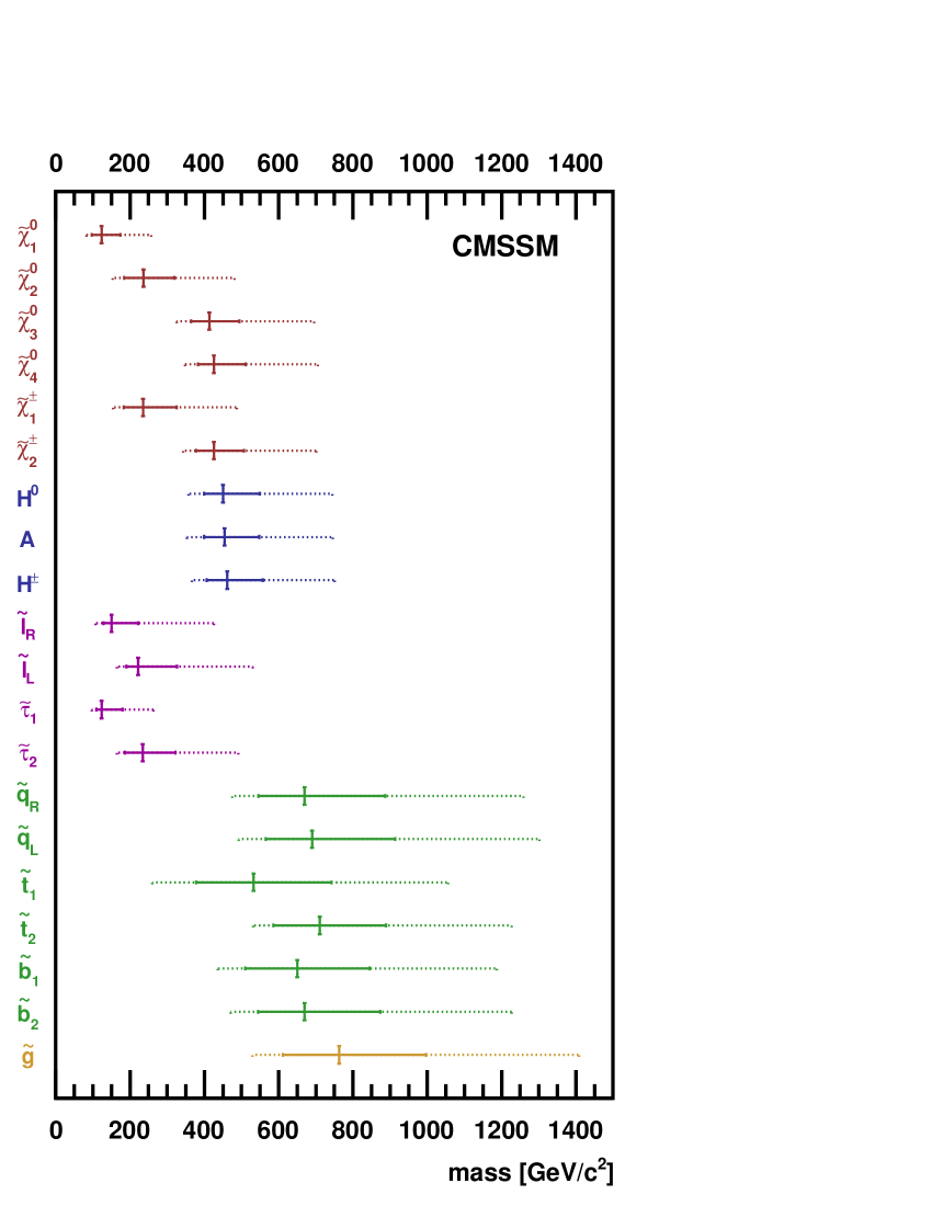
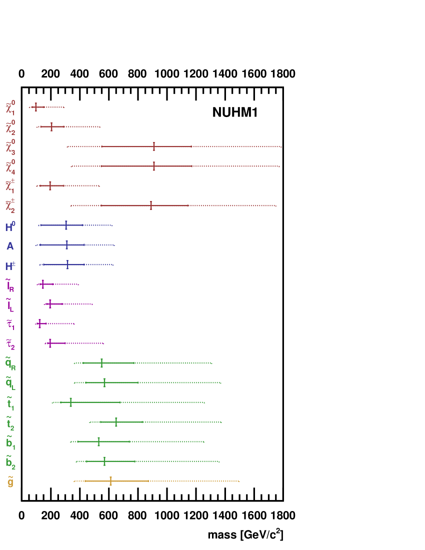
The central values of the masses of the supersymmetric partners of the quarks are slightly lighter than the gluino, as seen in Fig. 5. The difference between the gluino and the squark masses is sensitive primarily to . Since the preferred regions of the parameter space in both the CMSSM and the NUHM1 are in the -slepton coannihilation region where , makes only small contributions to the central values of the squark masses 131313However, this is not true in general, as we discuss in more detail later.. The SUSY partners of the left-handed components of the four lightest quarks, the , are predicted to be slightly heavier than the corresponding right-handed squarks, , as seen by comparing the mass ranges in Fig. 5. As in the case of the gluino, squark masses up to are allowed at the 3- level. Comparing the left and right panels, we see that the squarks are predicted to be somewhat lighter in the NUHM1 than in the CMSSM, but this difference is small compared with the widths of the corresponding likelihood functions.
Turning now to the likelihood functions for the mass of the lighter stop, , we find that it is shifted to values somewhat lower than for the other squark flavours. It can also be seen that the 2- range of its likelihood function differ from those of the gluino and the other squarks, reflecting the importance of scalar top mixing. We recall that this depends strongly on the trilinear soft SUSY-breaking parameter and the Higgs mixing parameter , as well as on the precise value of . As we discuss below, the favoured range of values of is quite circumscribed in the CMSSM, whereas a larger variation in is possible in the NUHM1. This has the effect of somewhat broadening the likelihood function for in the NUHM1.
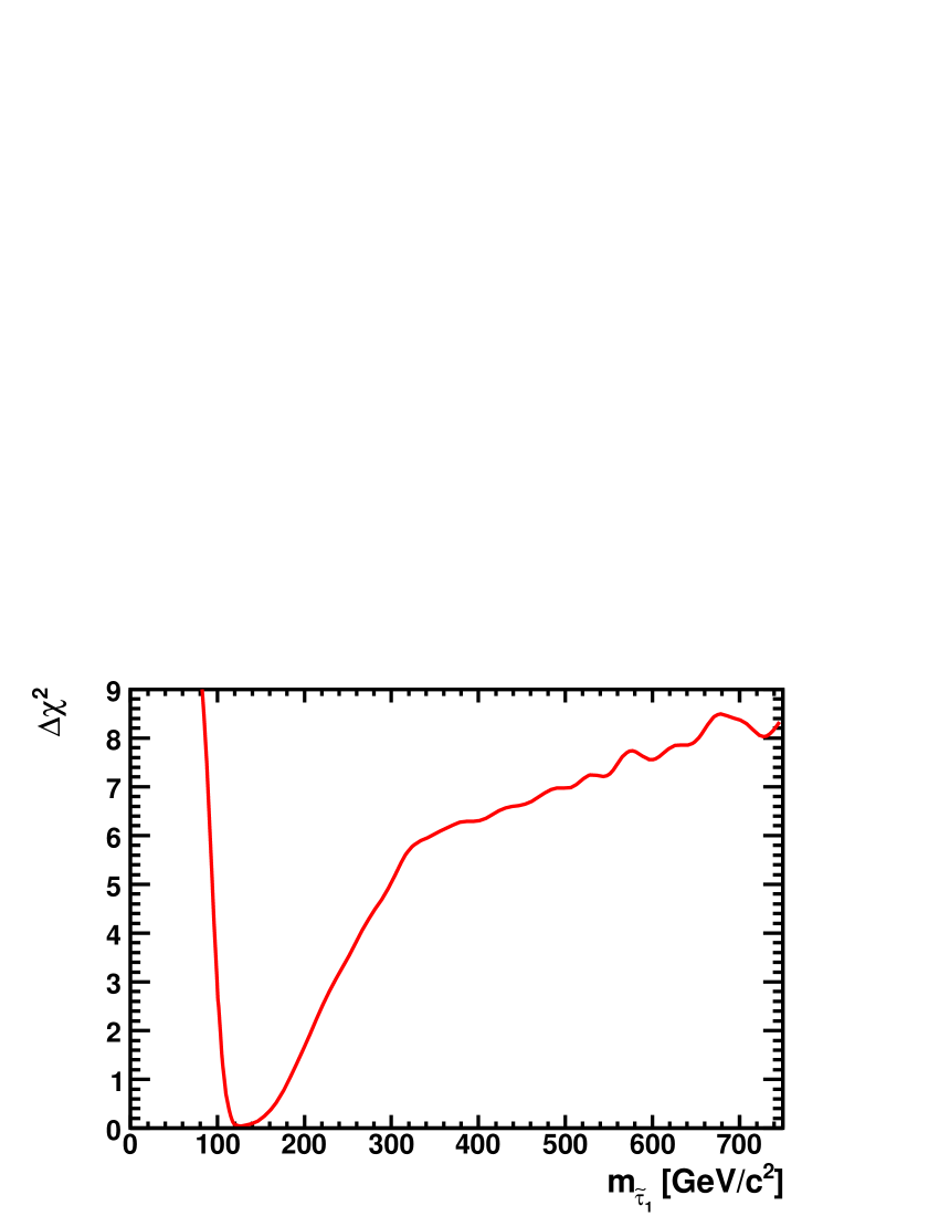
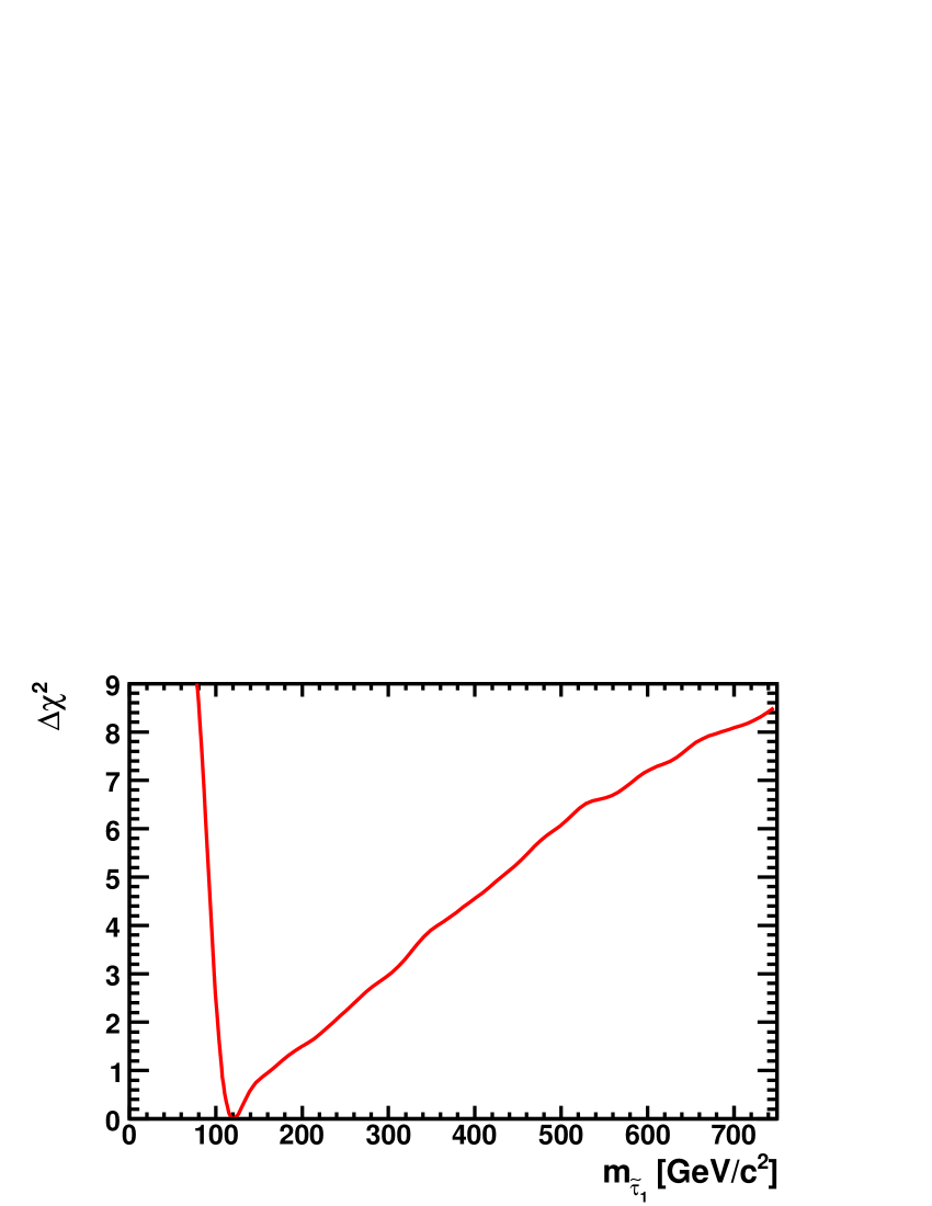
In the case of the lighter stau , see its range in Fig. 5 and its likelihood function in Fig. 6, the mass is very similar to that of the LSP in the coannihilation region, but this is not the case in the rapid-annihilation funnel region. The differences in the likelihood functions for the and the LSP , shown in Fig. 3, reflect the importance of this funnel region. In the case of the CMSSM (left panel of Fig. 6), the funnel region appears only at large values of that are relatively disfavoured. This is why the shape of the likelihood function differs significantly from that of the only at relatively large masses. In the case of the NUHM1 (shown in the right panel of Fig. 6), rapid annihilation is possible also for low , leading to larger values of than in the CMSSM also for relatively small values of .
The scalar taus as well as the other scalar leptons are expected to be relatively light, as can be seen in Fig. 5. They would partially be in the reach of the ILC(500) (i.e. with ) and at the 95% C.L. nearly all be in the reach of the ILC(1000) [131, 132]. This also holds for the two lighter neutralinos and the light chargino (In the NUHM1, small parts of the the 95% C.L. regions for the masses of the heavier stau and the light chargino are above .)
The left plot of Fig. 7 displays the likelihood functions for in the CMSSM (solid lines) and the NUHM1 (dashed lines) 141414We recall that, motivated by and BR(), we study only .. In the CMSSM, the values of and are fixed in terms of the other model parameters by the electroweak boundary conditions. Consequently, the range of values for is quite small in the CMSSM, and the magnitude of turns out to be relatively small. In the NUHM1, the much larger range of reflects the greater freedom in the Higgs sector. Solving the electroweak vacuum conditions for models with non-universal Higgs masses broadens the distribution151515Very large values of are disfavoured by the presence of deep charge- and colour-breaking minima [133, 134], but this constraint is not applied here., with the implications discussed above for the likelihood function for the . The right panel of Fig. 7 displays the likelihood functions for (see also the range in Fig. 5). The likelihood function in the CMSSM is again somewhat narrower than in the NUHM1, reflecting the influence of the electroweak boundary conditions. The best-fit value in the CMSSM is significantly higher than in the NUHM1. Values up to could be tested at the ILC(1000), i.e. the preferred regions of both models could be probed.
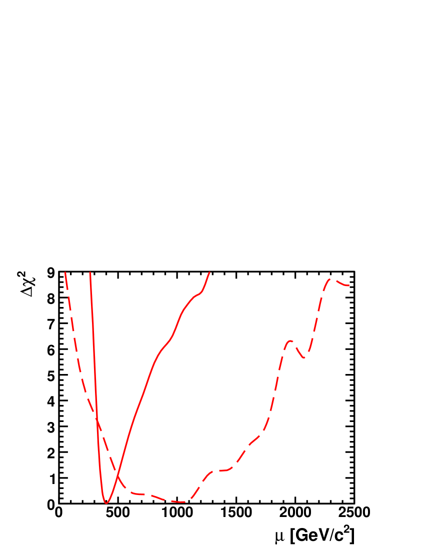
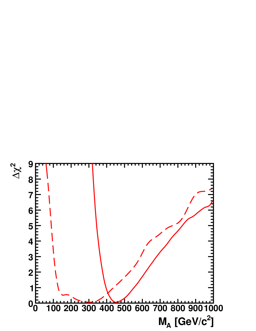
Fig. 8 displays the likelihood functions for . These are largely similar in the CMSSM and the NUHM1, with being favoured in both models.

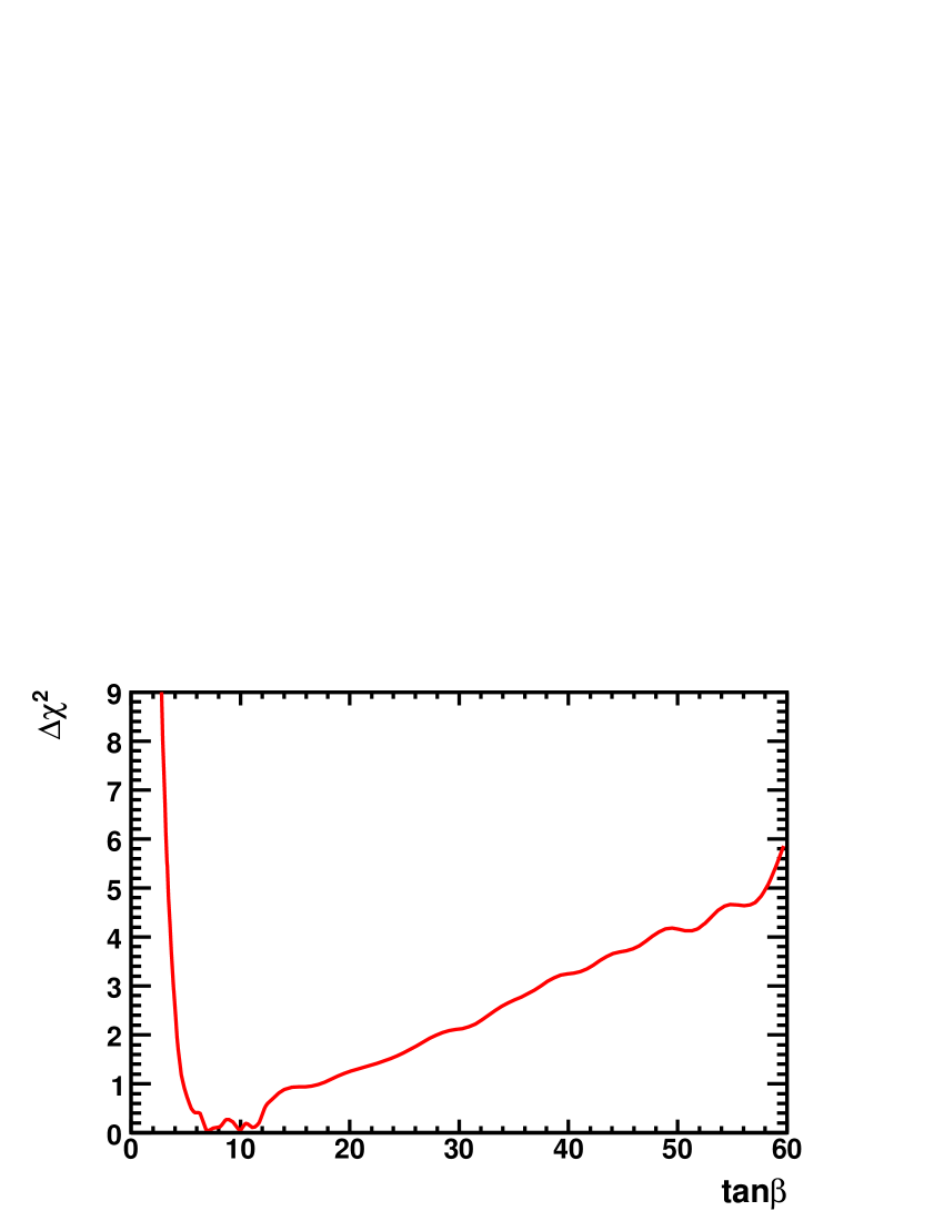
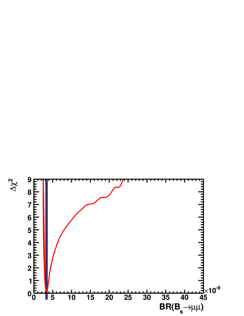
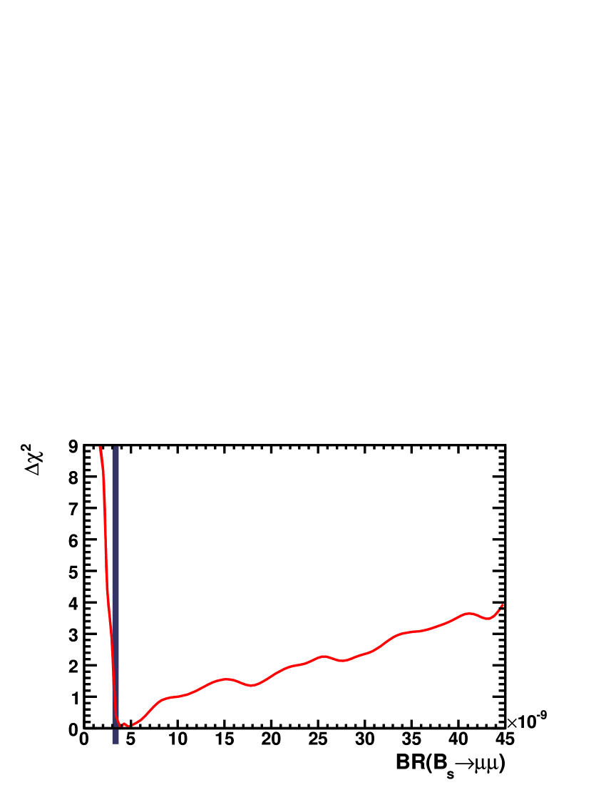
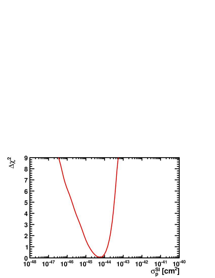
We turn now to the predictions for two other observables, namely BR() shown in Fig. 9 and the spin-independent -proton scattering cross section shown in Fig. 10 161616 The spin-independent -proton and -neutron scattering cross sections are very similar, and the spin-dependent scattering cross sections (not shown) are much further away from the prospective experimental sensitivity.. We see in the left panel of Fig. 9 that values of the BR() similar to that in the SM are favoured, particularly for the preferred lower values of . However, large deviations from the SM prediction (indicated by the vertical lines, which include the theoretical uncertainty) are still possible at the 3- level. The picture in the NUHM1 is completely different, since the function is quite flat, with no significant penalty for substantial deviations from the SM prediction, and very large values of the branching ratio being allowed at the 2- level. The difference is largely due to the fact that smaller masses of the heavier Higgs bosons are permitted in the NUHM1. A large value of BR() would be a promising harbinger of SUSY at the LHC, and would favour a priori the NUHM1 over the CMSSM. Assuming the SM value, i.e. , it has been estimated [135] that LHCb could observe this process at the 5 level within a few years of running. This makes this process a very interesting probe of SUSY that could help to distinguish between different models.
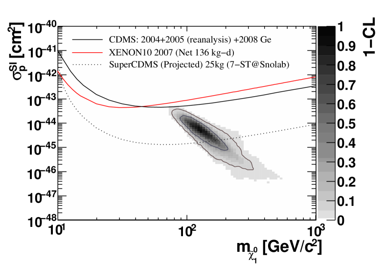
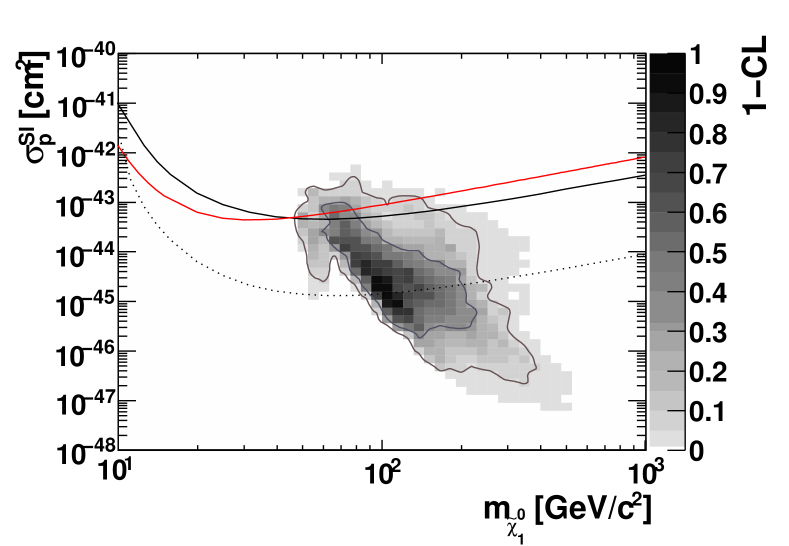
The value of shown in Fig. 10 is calculated assuming a -N scattering term MeV: plausible values range between about 45 and 80 MeV, and increases quite rapidly with [136, 137, 138]. We see in Fig. 10 that values of the -proton cross section pb are expected in the CMSSM, and that much larger values seem quite unlikely. On the other hand, in the NUHM1, though the best-fit value of the cross section is somewhat lower, a much larger range is possible 171717No scaling of the cross-section was done here to account for regions where falls below the WMAP range, but such points pay a penalty.. Hence, detection of dark matter with a cross section much larger than pb cm2 would also be a good diagnostic for discriminating between the NUHM1 and the CMSSM. The present best upper limits on from the CDMS [139] and Xenon10 [140] experiments are at the pb level 181818Assuming a local LSP density of 0.3 GeV/cm3, which is subject to astrophysical uncertainties., and the planned experiments should be sensitive down to below the pb level [141, 142].

5 Correlations between Sparticle Masses and with other Observables
We now discuss in more detail some of the correlations between sparticle masses and observables, starting with the LSP mass, , and the gluino mass, , shown in Fig. 11 191919For one-dimensional scans, we continue to quote up to 9 units in , which corresponds to . For two-dimensional confidence level contour plots, we quote instead of the ; the blue (red) lines in the plots correspond to %, and the white regions correspond to , or units.. We expect a very strong correlation, since the value of largely controls both masses. However, in both cases there are radiative corrections that enter when making the transition from the SUSY-breaking parameters defined using the prescription to the on-shell masses, that depend on the other MSSM parameters. Moreover, the LSP is not a pure Bino, and the mixing with other neutralino states depends on the value of , in particular. Indeed, we see in Fig. 11 a very strong correlation in the CMSSM (left panel), which is not quite so strong for the NUHM1 (right panel). Moreover, in the latter case we notice a small (grey) island of parameters where is substantially lower than one would have expected for the corresponding value of . These few examples have a Higgsino-like LSP, and have relatively small likelihoods.
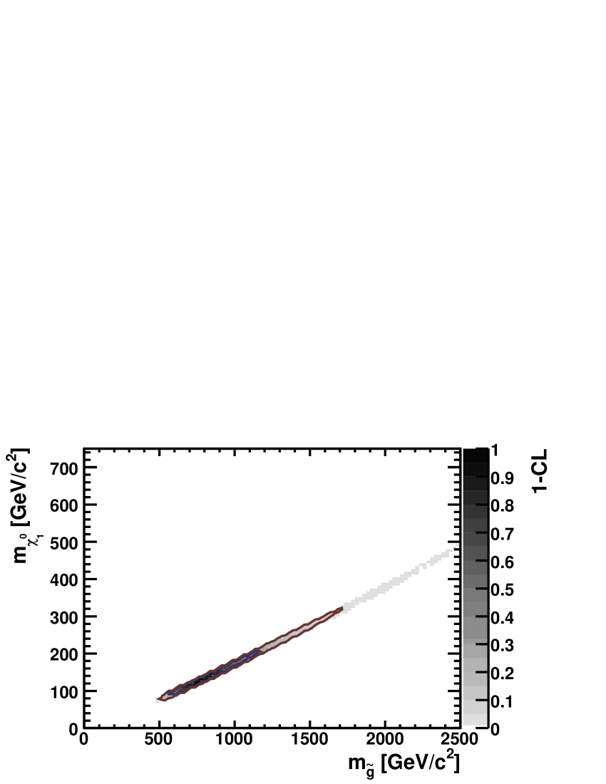

A corollary of the correlation between and seen in Fig. 11 is the relation between the mass scale of the heavy supersymmetric particles [143] that might be discovered at the LHC with the threshold for producing the lighter sparticles that might be measured at a future linear collider. If one observes a gluino at a certain mass scale (or establishes a lower limit on its mass), according to Fig. 11 one will have, within the CMSSM or the NUHM1, a lower bound on the threshold for pair-producing observable sparticles at a linear collider, 202020The lightest neutralino might then be visible in the channel [144, 145, 146].. The relevant may be read directly off the vertical scale of Fig. 11. This is in general related to by a simple, universal numerical factor, the only exception being the small island (which has a rather low likelihood) of models with unusually low in the NUHM1, mentioned earlier and seen in the right panel of Fig. 11.
In principle, the masses of the squark partners of the five lightest quarks depend on as well as . However, as seen in Fig. 12, they are also very highly correlated with , reflecting the fact that in the favoured regions of the CMSSM and the NUHM1, and also the fact that the sensitivities of to are intrinsically smaller than that to . That said, we see that the correlations of with are slightly weakened in the CMSSM (left panels) at large , reflecting the appearance of the rapid-annihilation funnel with relatively large at large and . The greater width of the correlations in the NUHM1 (right panels) at small , compared to the CMSSM, reflects the possibility of greater due to the appearance of a rapid-annihilation funnel at smaller values of and than in the CMSSM.

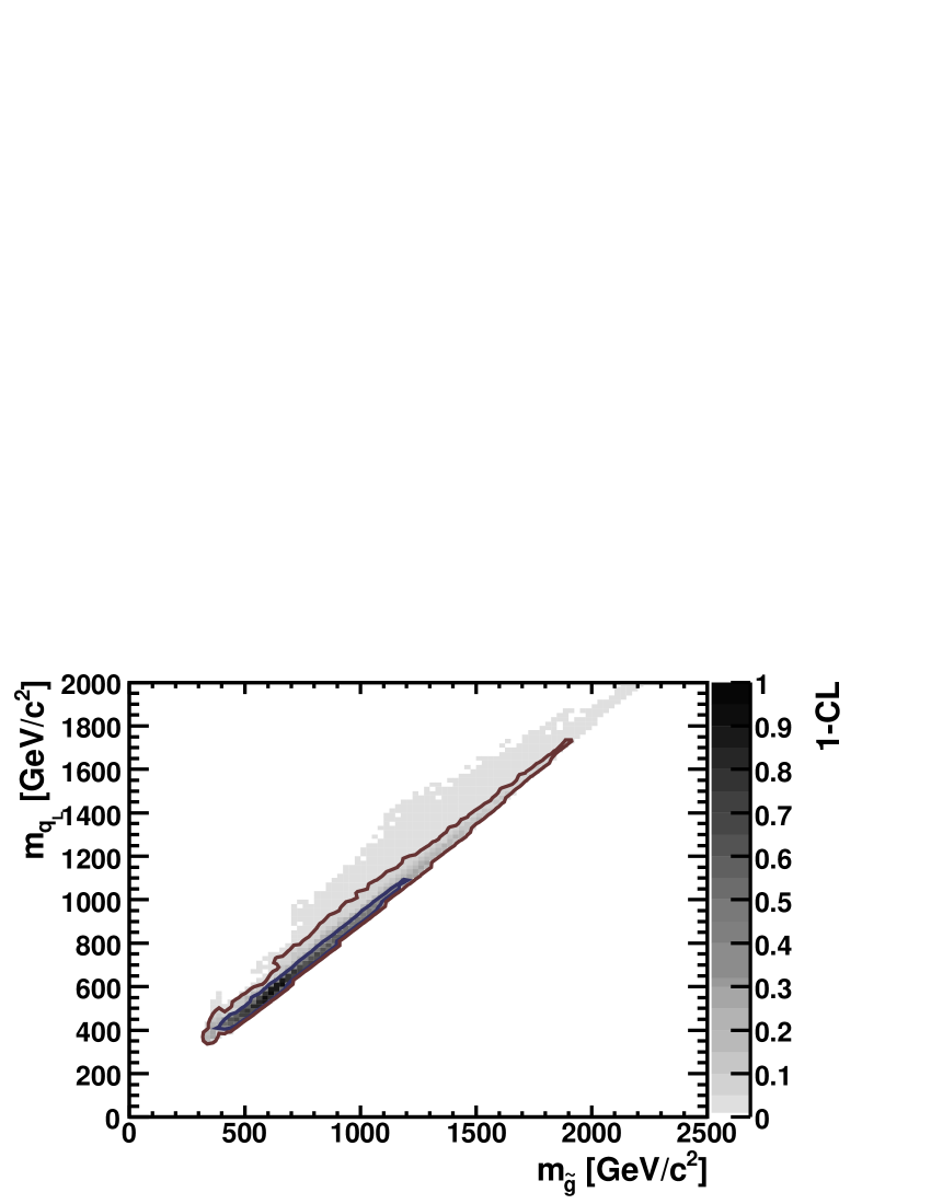
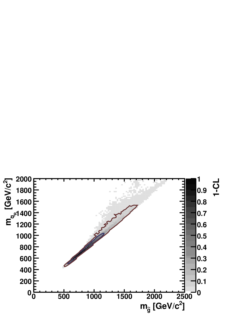
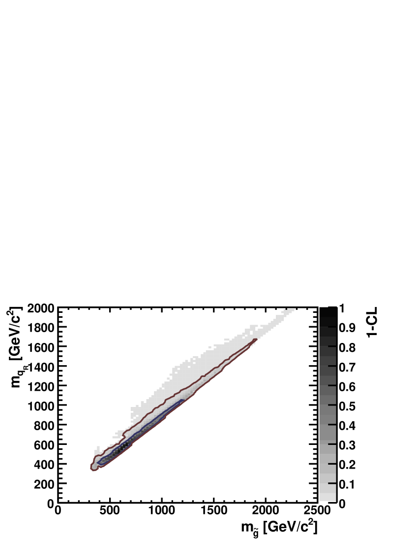
These effects are more visible in Fig. 13, where we plot the differences between the gluino and squark masses in the CMSSM (left plots) and in the NUHM1 (right plots). In the CMSSM, in the the cases of both the (upper left panel) and (lower left panel), we see that the squarks are always lighter than the gluino if is itself light. However, if , although is still favoured, this is not necessarily the case, and becomes a possibility, because of the larger values of that occur in the rapid-annihilation funnel that appears as and increases. In the case of the NUHM1 (right panels), is a possibility also at low , thanks to the possible appearance of a rapid-annihilation funnel also at low .
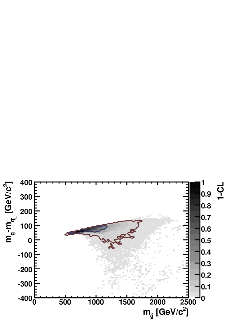
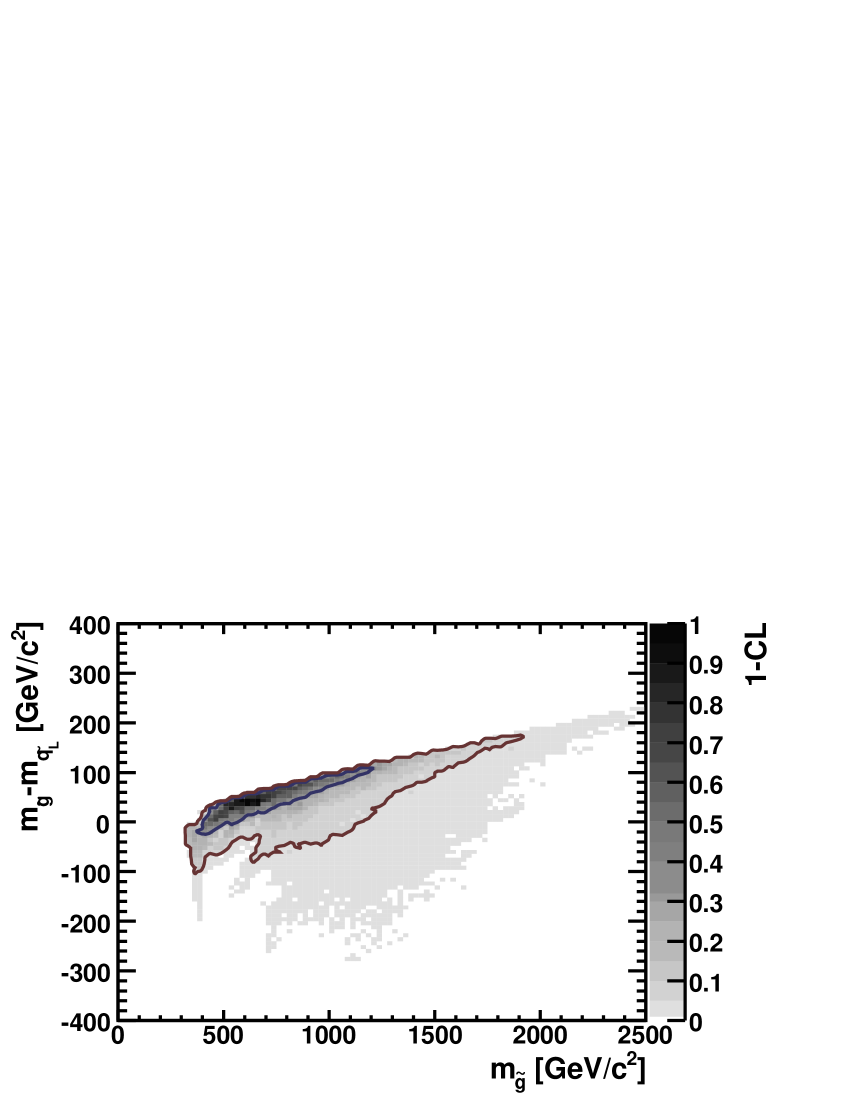
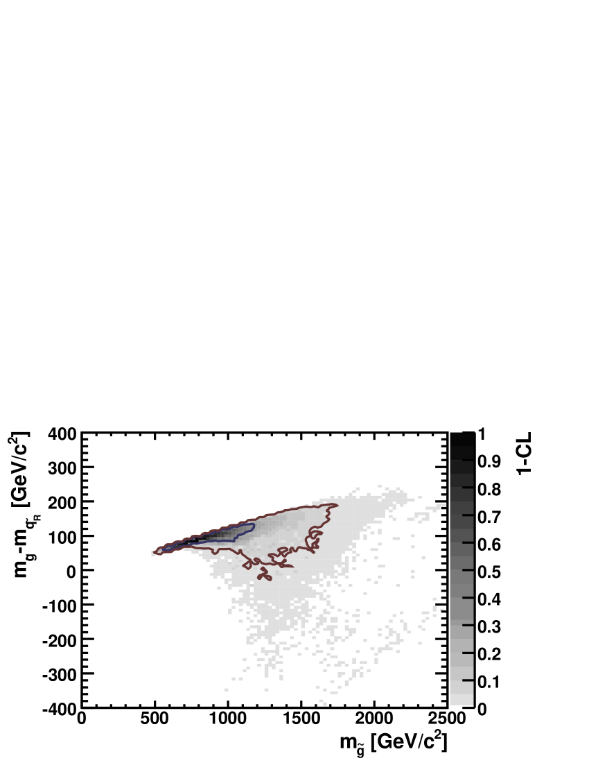

Fig. 14 displays the correlation between and , which is somewhat weaker than the correlation between and the other squark masses. This is because, in addition to sharing the dependence on with the other squarks, is sensitive, as commented earlier, to the value of as well as and . We recall further that the preferred range of is broader in the NUHM1 than in the CMSSM, which explains why in this model the preferred range of is broader for intermediate values of .
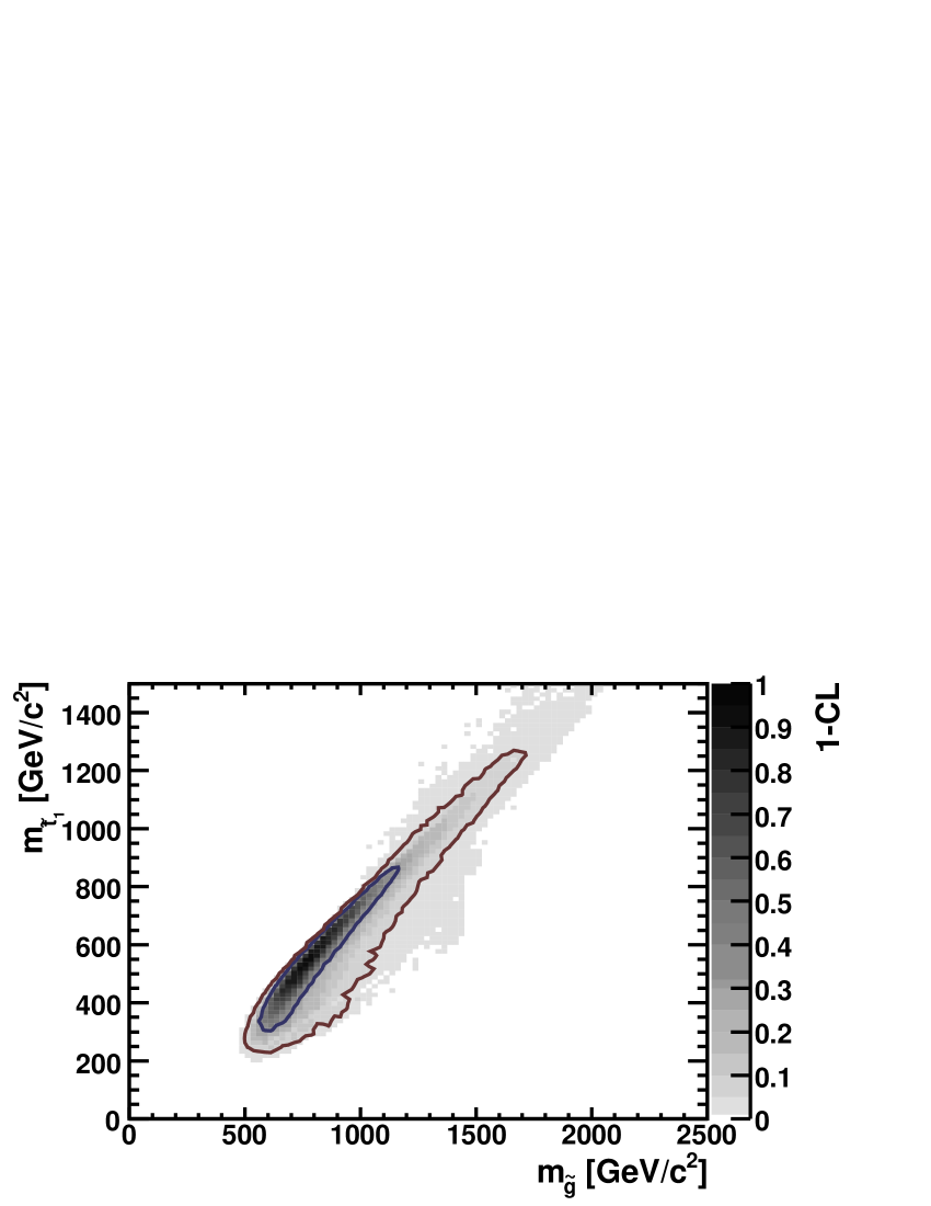
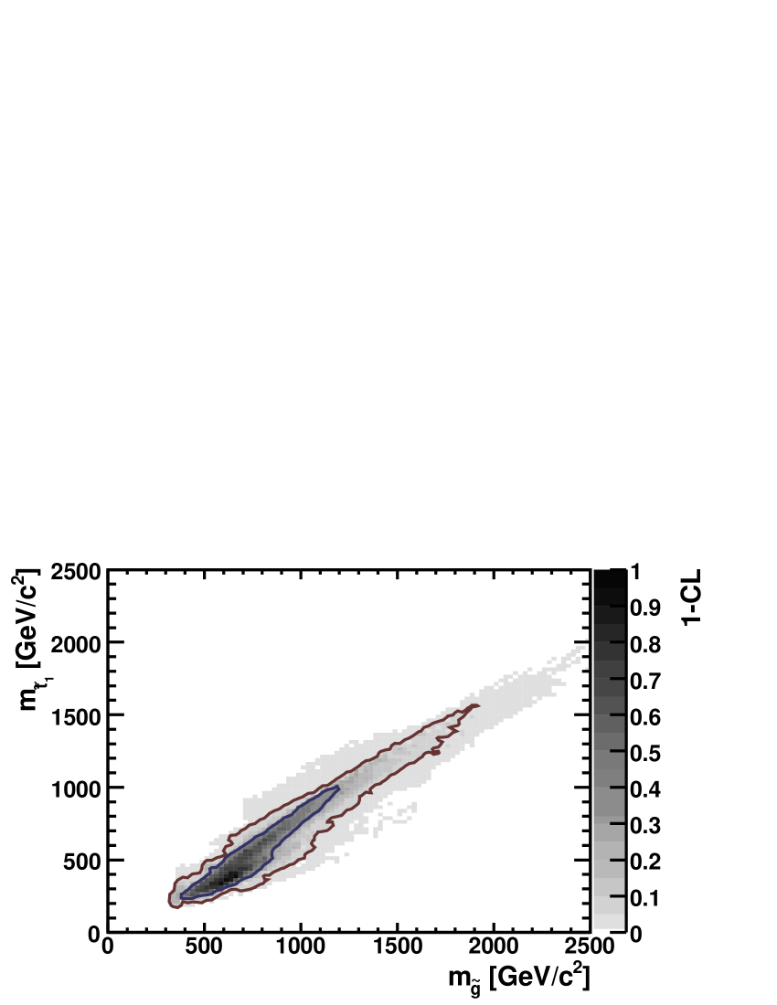
Fig. 15 displays the correlation between and , which is generally proportional to the LSP mass, as discussed earlier. The - correlation is strikingly different in the CMSSM (left panel) and the NUHM1 (right panel). The tight correlation in the CMSSM reflects the fact that the favoured part of the parameter space is in the - coannihilation region, where the - mass difference is very small. On the other hand, in the NUHM1, as already commented, there are favoured regions away from the coannihilation region, where rapid annihilation through direct-channel poles keeps the relic density within the WMAP range.

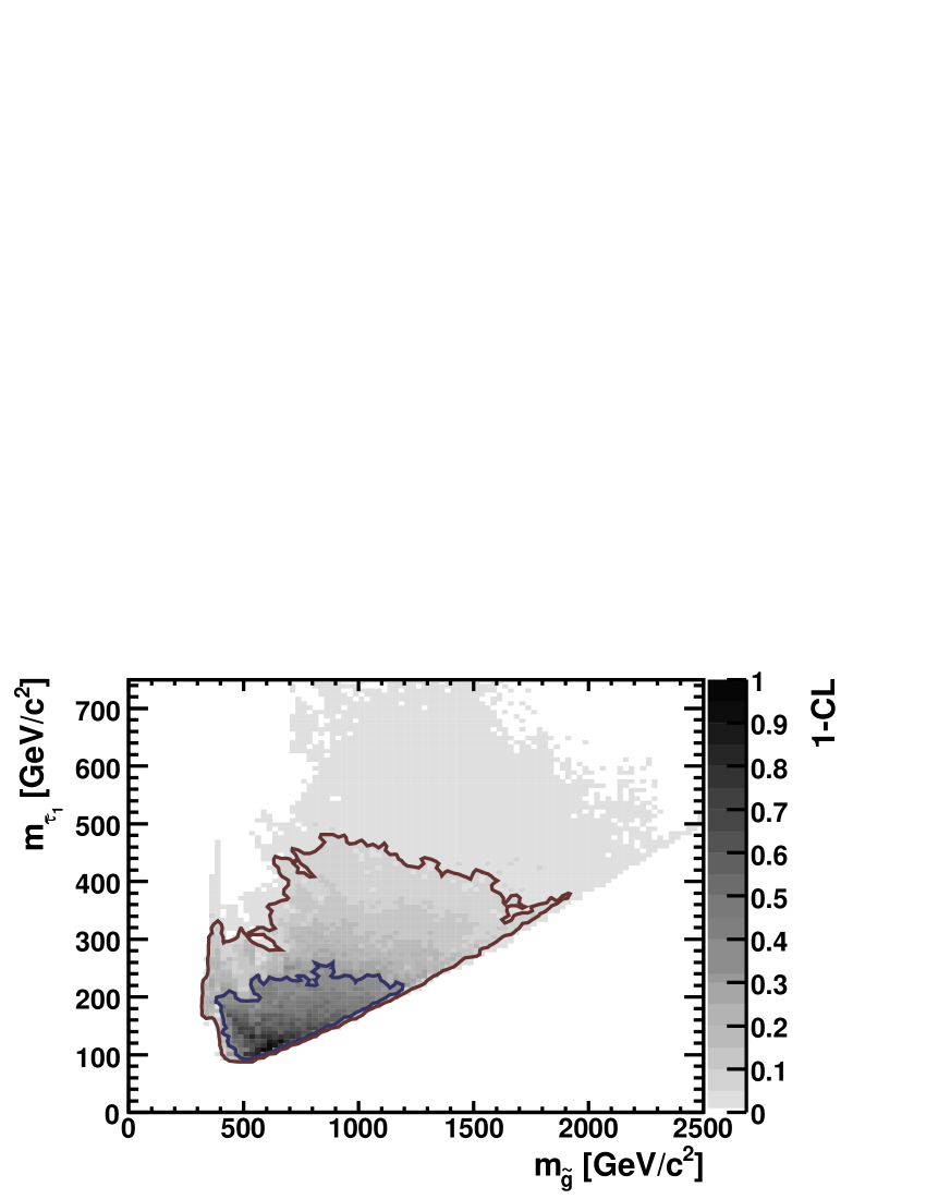
Fig. 16 demonstrates explicitly the big contrast between the behaviours of the - mass difference in the CMSSM (left panel) and the NUHM1 (right panel). We see that in the CMSSM small mass differences are always favoured, and are mandatory for LSP masses , whereas larger mass differences are possible for LSP masses , as the rapid-annihilation funnel opens up. However, in the NUHM1 large mass differences are possible for all LSP masses, particularly for LSP masses . This means that, whereas in the CMSSM the ‘visible’ pair-production threshold at the ILC may be only slightly higher than the ‘invisible’ pair-production threshold, it may be considerably higher in the NUHM1, namely at the 95% C.L.. This is a potentially crucial signature for distinguishing the NUHM1 from the CMSSM.
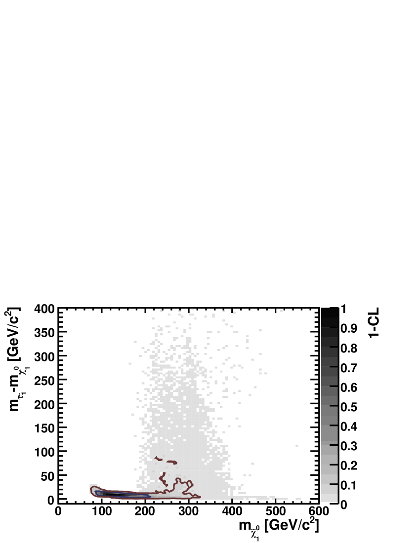

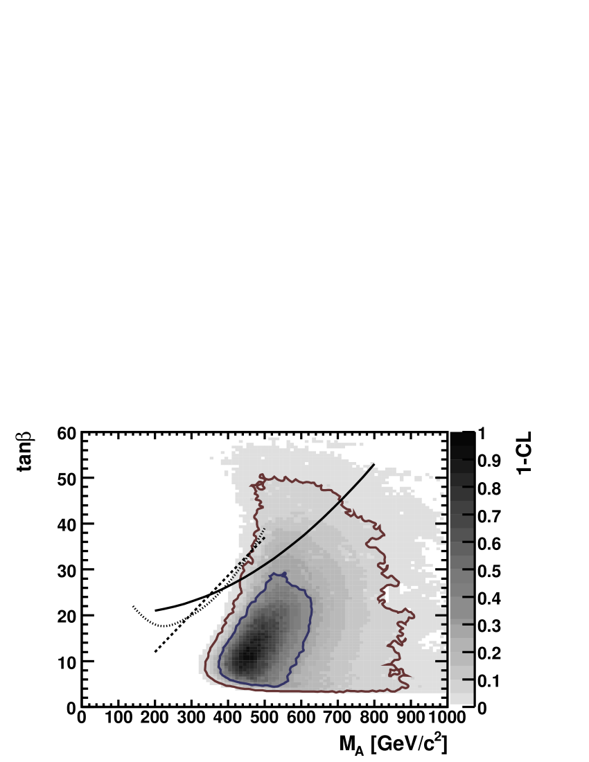
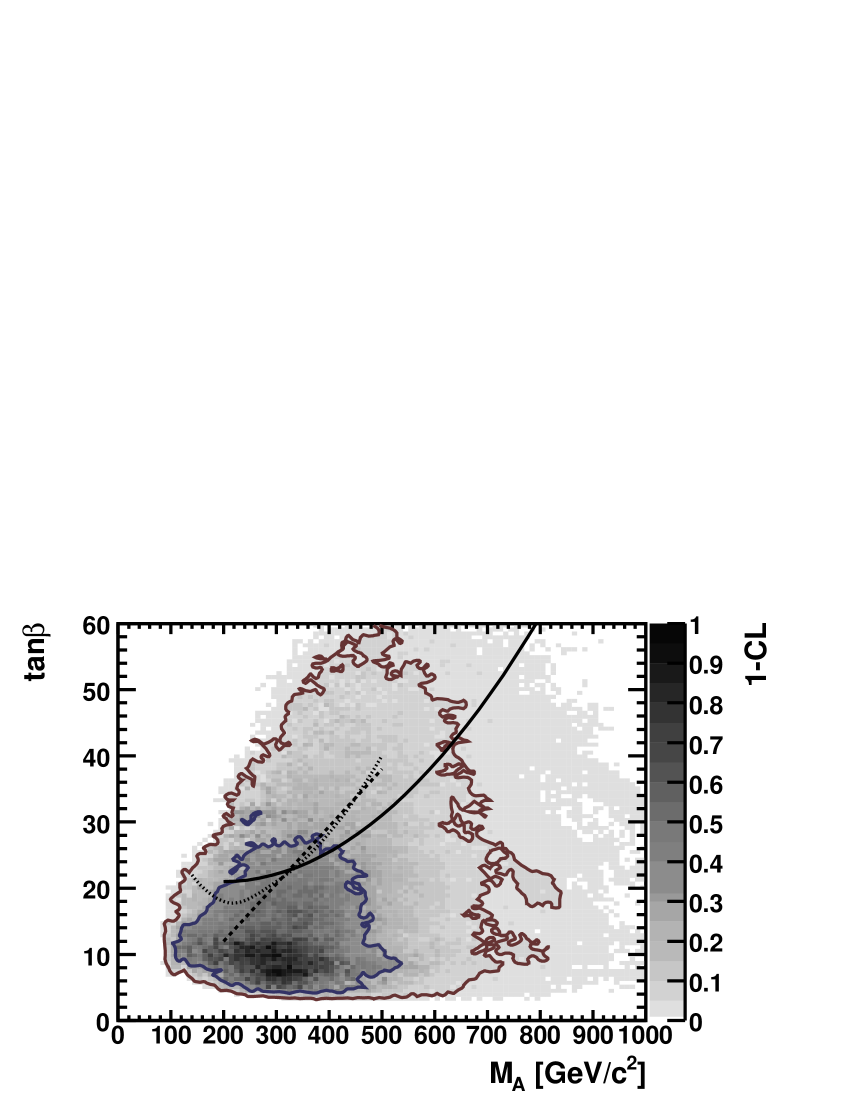
Fig. 17 displays the favoured regions in the planes for the CMSSM and NUHM1. We see that they are broadly similar, with little correlation between the two parameters. planes in certain benchmark scenarios have often been used in the past to analyze the prospects for discovering heavy Higgs bosons at the LHC [147, 148]. Most of these analyses have been done in the context of scenarios that do not take the relic-density constraint into account, for exceptions see [34, 35]. The Higgs discovery contours determined in the various benchmark scenarios cannot directly be applied to the planes in Fig. 17 displaying our fit results for the CMSSM and the NUHM1. In order to assess the prospects for discovering heavy Higgs bosons at the LHC in this context, we follow the analysis in [149], which assumed 30 or 60 fb-1 collected with the CMS detector. For evaluating the Higgs-sector observables including higher-order corrections we use the soft SUSY-breaking parameters of the best-fit points in the CMSSM and the NUHM1, respectively. We show in Fig. 17 the 5- discovery contours for the three decay channels (solid lines), (dashed lines) and (dotted lines). The parameter regions above and to the left of the curves are within reach of the LHC with about 30 fb-1 of integrated luminosity. We see that most of the highest-CL regions lie beyond this reach, particularly in the CMSSM. At the ILC(1000) masses up to can be probed. Within the CMSSM this includes the best-fit point, and within the NUHM1 nearly the whole 68% C.L. area can be covered.
We display in Fig. 18 the correlations between and in the CMSSM and in the NUHM1. In the former case, the electroweak boundary conditions fix , and the effect is to force . However, becomes essentially a free parameter in the NUHM1, and values smaller than become possible also. On the other hand, there is a narrow strip where which is disfavoured because there rapid direct-channel annihilation suppresses the relic density below the range preferred by astrophysics and cosmology. The points with are a qualitatively new possibility opened up within the NUHM1 as compared to the CMSSM, and extend to relatively large values of .
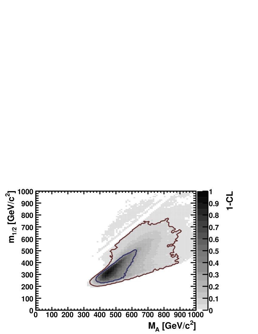
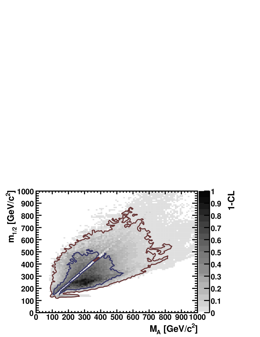
Fig. 19 displays the correlation between and the BR(). As seen previously, in the CMSSM the preferred values of the branching ratio are very close to the value in the SM, though somewhat larger values may occur at large , which however have a lower likelihood. The situation is completely different in the NUHM1, where much larger values of the branching ratio for BR() are possible, even if . This increase reflects the possibility that may be considerably smaller than in the CMSSM. The upper right corner of the NUHM1 plot, i.e., simultaneous large and large BR(), is disfavoured because it would give rise to values of BR() that are too small.
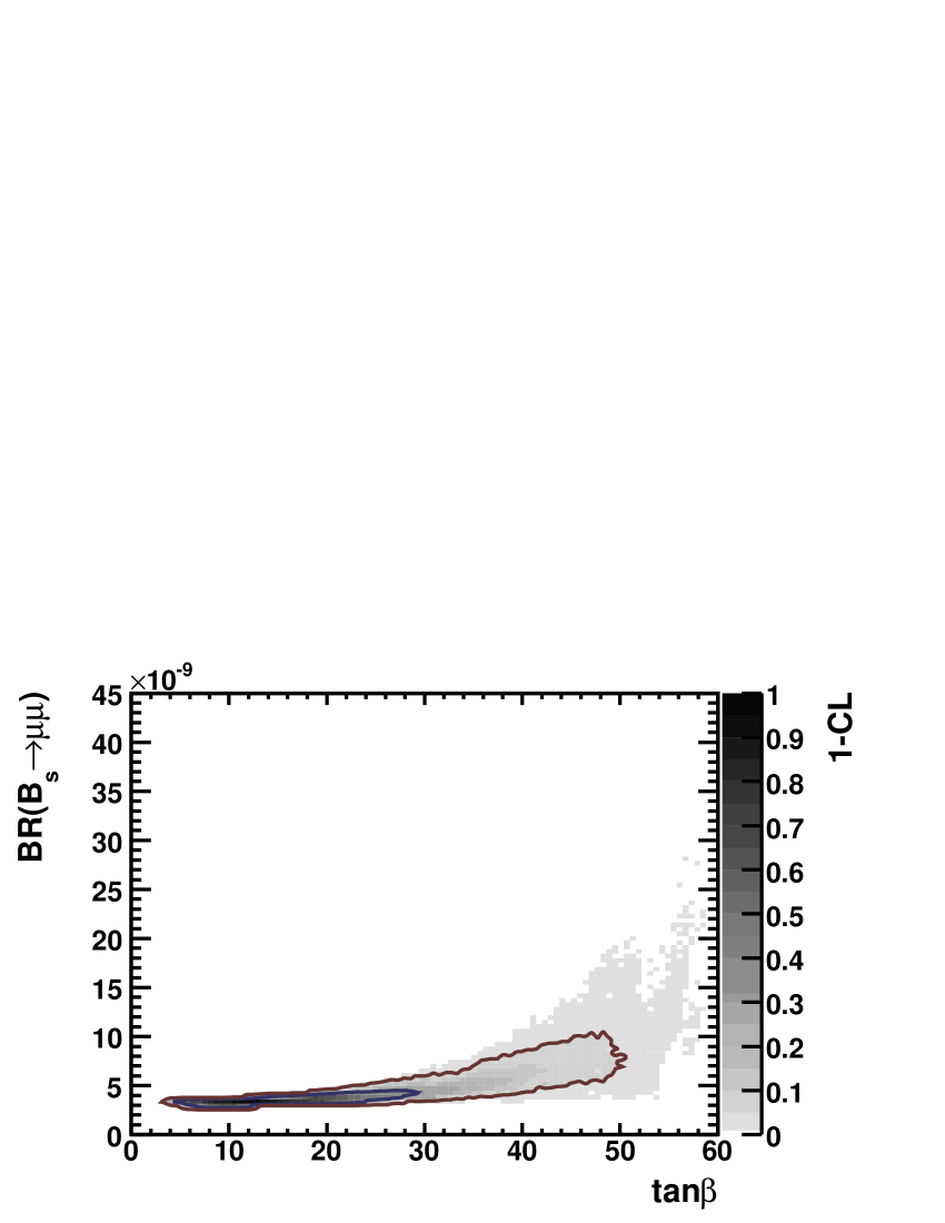
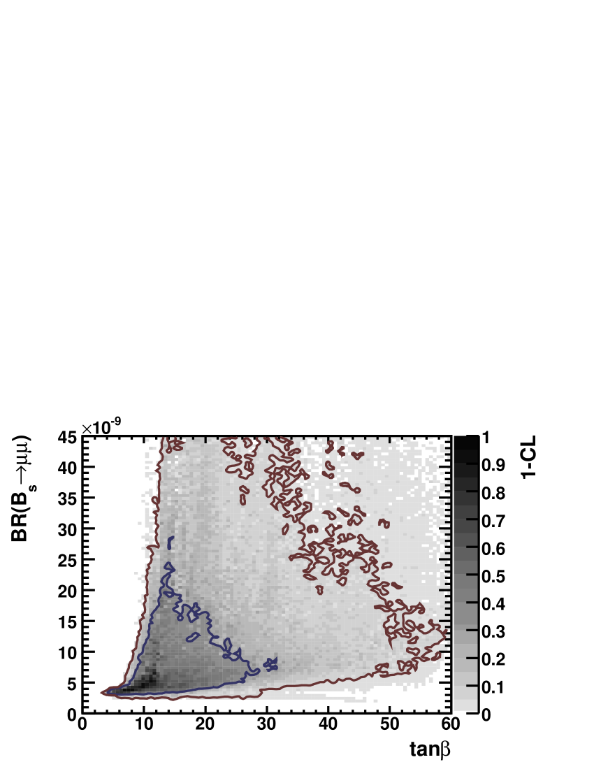
Fig. 20 displays the preferred range of the spin-independent DM scattering cross section (calculated assuming a -N scattering term MeV) as a function of . In the case of the CMSSM, we see that the expected range of lies mainly between the present experimental upper limits (solid lines) [139, 140], which start to touch the preferred region, and the projected sensitivity of the SuperCDMS experiment (dashed line) [142], which should cover the preferred region. As noted earlier, these experimental constraints were not applied in our analysis. The uncertainty in and the astrophysical uncertainties in the local dark matter density (which are difficult to quantify), preclude including the value of in the likelihood analysis presented here. This region is in good agreement for neutralino masses between 100–300 GeV with that found in [63], where a recent scan (without likelihood information) was performed.
As already commented, the range in the NUHM1 is larger than in the CMSSM. We see in Fig. 20 that the larger cross-section values occur, as expected, for small , in particular in the small island of Higgsino-like DM that appears close to the 95% C.L. for . If , the allowed range of the cross section is larger than in the CMSSM because of the wider range of possible values of as found in [63] for this neutralino mass range, and the present experimental sensitivity is already below the values of found for some favoured NUHM1 parameter values assuming the nominal values of and the local LSP density. The smallest values of the cross section occur when , in models close to the 95% C.L. limit for the NUHM1, which have larger than in the CMSSM. In general, we see that whereas the favoured values of are close to the present experimental upper limits [155] in both the CMSSM and the NUHM1, there is a greater possibility in the NUHM1 that the cross section may lie beyond the projected sensitivity of SuperCDMS [142].
6 Dropping Constraints
6.1 Dropping the Constraint
We have stressed above that the results in the previous section are strongly dependent on the implementation of the constraint. In particular, we have displayed in Fig. 2 above the likelihood functions for in the CMSSM (left) and the NUHM1 (right) both with the constraint imposed (solid) and without it (dashed). We now discuss in more detail the effect of dropping the constraint completely, calculating a new with no contribution from .
The function obtained for in the CMSSM without the constraint, shown in the left panel of Fig. 2, is much flatter than the corresponding function obtained with the constraint. Nevertheless, we see non-trivial features in the function. One is that the location of the CMSSM global minimum is very similar to the case with the constraint applied. We recall that the rise in the function at small is determined essentially by the and BR() constraints, with not playing a role. However, it is perhaps surprising that the other constraints cause to rise until , where . However, we see in Table 2 that, in addition to , several other constraints favour the best-fit CMSSM point over points with , including BR(), , and . Continuing to larger in the left panel of Fig. 2, we see that decreases again slightly, but that still .
Similar features are seen in the function obtained for in the NUHM1 without the constraint, shown in the right panel of Fig. 2. Again, the value of at the best-fit NUHM1 point is very similar, whether is included or not, and again at large . However, there is no intermediate hump at analogous to that in the CMSSM, reflecting the greater freedom in the NUHM1 to adjust parameters so as to obtain a lower value of .
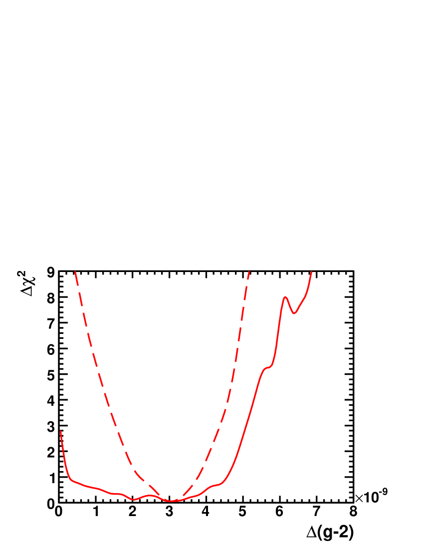
A corollary of the observations in the previous paragraphs is that, at some level, the other constraints favour a non-zero supersymmetric contribution to . This is indeed visible in Fig. 21, where we see the predicted values of the contributions of supersymmetric particles to in the CMSSM (left) and the NUHM1 (right). We show the functions only for positive contributions to , since our points were all chosen to have . Nevertheless, the fact that the minima of the distributions are for is non-trivial, because it reflects the above observation that large values of the sparticle masses are disfavoured, and the order of magnitude prediction for agrees with estimates based on low-energy data.

6.2 Dropping the BR() Constraint
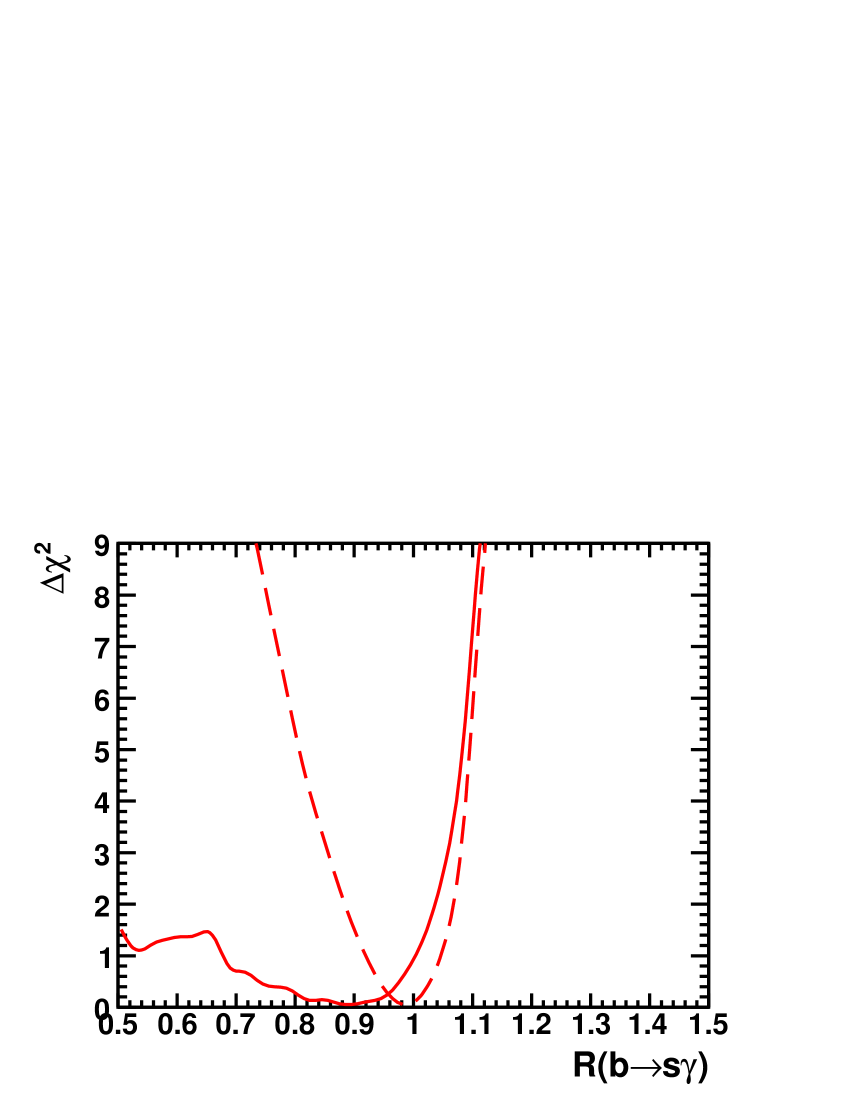
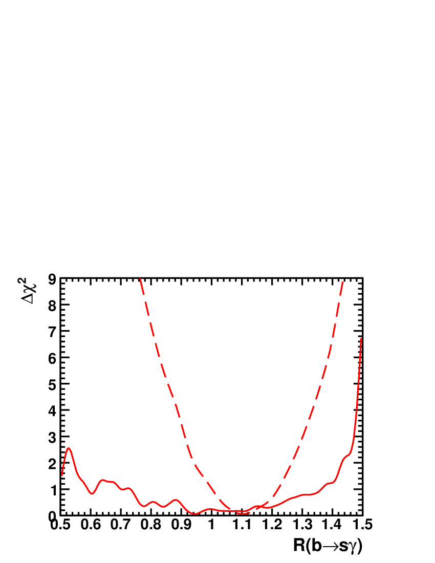
We display in Fig. 22 the effects on the CMSSM and NUHM1 fits (left and right panels, respectively) of omitting the BR() constraint from the global fit, as obtained by calculating a new with no contribution from BR(). In both models, we see that the predictions for BR() based on the other constraints (solid lines) are not very precise. The best-fit values for BR() are in both models quite close to the SM and hence the experimental value, but the CMSSM permits much smaller values, and both larger and smaller values are allowed in the NUHM1 with relatively small increases in .
The converse statement is that applying the BR() constraint does not impose a large price on the global minimum. This is apparent from Table 2, where we saw that BR() contributes about to the total in the CMSSM and yields a negligible contribution in the NUHM1. There is no tension between BR() and the other constraints.
6.3 Dropping the Constraint
One of the most exciting predictions of the CMSSM and the NUHM1 is the existence of a cold dark matter candidate in the form of the LSP, which we assume here to be the lightest neutralino [150]. It is natural to take the next step, and ask whether these models predict a relic LSP density that is close to the experimental value of the cold dark matter density. This density is determined with an accuracy of a few percent, and an comparable accuracy in the prediction based on the other available experimental constraints will be difficult. This will improve if (when) the LHC discovers SUSY and its parameters are measured more accurately at an linear collider [65, 151, 152, 57].
Nevertheless, calculating a new with no contribution from , it is interesting to see in Fig. 23 that both the CMSSM (left) and NUHM1 (right) favour ranges of values that include the measured values of the cold dark matter density. In the case of the CMSSM, the prediction for (solid line) is within an order of magnitude above and below the measured value at the level . This is also true in the NUHM1 above the measured value, but the relic LSP density could be two or more orders of magnitude below the measured value with . This is because there is a possibility that the relic density may be suppressed by rapid annihilation through direct-channel Higgs poles in the region of relatively low and in the NUHM1 that is favoured by the other constraints, notably .
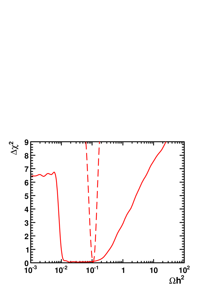
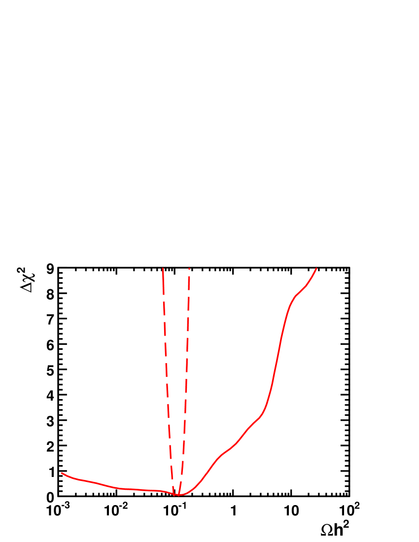
The converse statement is that applying the constraint also does not impose a large price on the global minimum. In fact, in both the CMSSM and the NUHM1, and therefore has not been listed in Table 2. As in the case of BR(), there is no tension between and the other constraints.
6.4 Dropping the Constraint
We have already commented on the effect on the likelihood function for of dropping the LEP constraint, see Fig. 3, and on the prediction for itself, see Fig. 4. We now discuss in more detail the likelihood functions for within the CMSSM and NUHM1 frameworks obtained when dropping the contribution to from the direct Higgs searches at LEP, shown in the left and right panels of Fig. 24, respectively. The left plot updates that for the CMSSM given in [53].
It is well known that the central value of the Higgs mass in a SM fit to the precision electroweak data lies below 100 GeV [153, 73], but the theoretical (blue band) and experimental uncertainties in the SM fit are such that they are still compatible at the 95% C.L. with the direct lower limit of 114.4 GeV [106] derived from searches at LEP. In the case of the CMSSM and NUHM1, one may predict on the basis of the underlying model parameters, with a 1- uncertainty of 1.5 GeV [102], shown as a red band in Fig. 24. Also shown in Fig. 24 are the LEP exclusion on a SM Higgs (yellow shading) and the ranges that are theoretically inaccessible in the supersymmetric models studied (beige shading) 212121It is apparent that the current Tevatron exclusion [154] of a range between 160 and 170 GeV does not impact supersymmetric models.. The LEP exclusion is directly applicable to the CMSSM, since the couplings are essentially indistinguishable from those of the SM Higgs boson [66, 67], but this is not necessarily the case in the NUHM1, as discussed earlier in this paper.
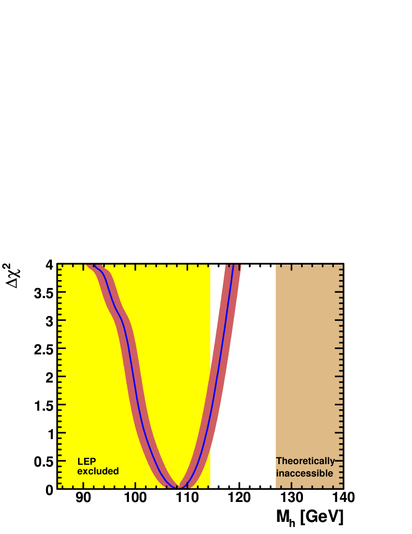
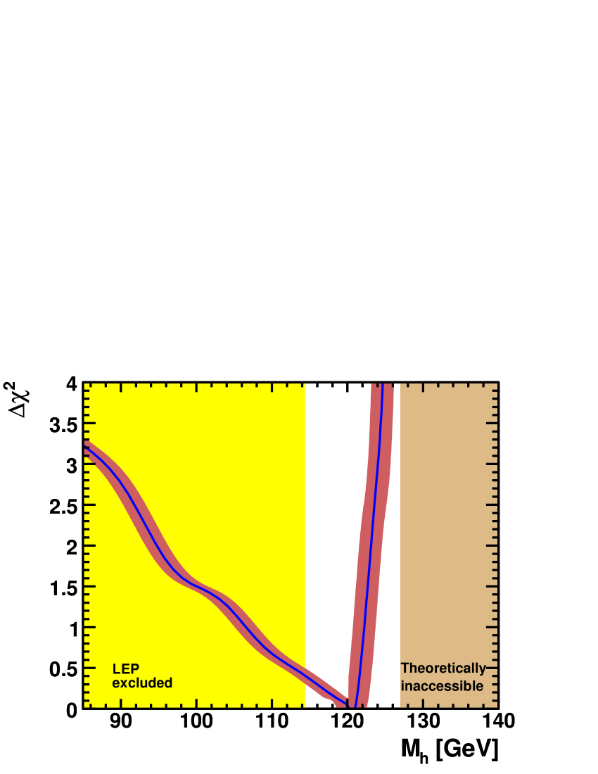
In the case of the CMSSM, we see in the left panel of Fig. 24 that the minimum of the function occurs below the LEP exclusion limit. While the tension between the function for arising from the CMSSM fit and the LEP exclusion limit has slightly increased compared to the earlier analysis performed in [53], the fit result is still compatible at the 95% C.L. with the search limit, similarly to the SM case. As we found in the analysis performed above, a global fit including the LEP constraint has acceptable . In the case of the NUHM1, shown in the right panel of Fig. 24, we see that the minimum of the function occurs above the LEP lower limit on the mass of a SM Higgs. Thus, within the NUHM1 the combination of all other experimental constraints naturally evades the LEP Higgs constraints, and no tension between and the experimental bounds exists.
7 Conclusions
We have presented in this paper detailed results from global fits to available experimental and cosmological data within the CMSSM and NUHM1, using a frequentist approach. As already reported in [4], we find relatively small values of the key input SUSY-breaking parameters and in both models. Moreover, the values for these parameters are quite similar in the two models, indicating that the predictions are relatively robust and do not depend strongly on the details of the Higgs sector.
We have presented details of the likelihood functions for individual sparticle masses and the correlations between them. As noted in [4], the particle spectra are similar in the two models, the most prominent differences being in the masses of the heavier Higgs bosons and , which are lighter in the NUHM1, and the heavier neutralinos and chargino, which are lighter in the CMSSM. These differences reflect the greater freedom in varying the parameters of the Higgs sector in the NUHM1. The favoured values of the particle masses in both models are such that there are good prospects for detecting supersymmetric particles even in the early phase of the LHC running with reduced centre-of-mass energy and limited luminosity and for observing supersymmetric particles and possibly the whole Higgs boson spectrum at a 1 TeV collider (the latter refers in particular to the case of the NUHM1).
We find striking correlations between the different sparticle masses in both the CMSSM and the NUHM1. This reflects the fact that the dominant contributions to most of the sfermion masses are those due to , implying that most sparticle masses are tightly correlated with those of the gluino and the LSP. These correlations imply that, if the gluino is discovered at the LHC and its mass determined by a combination of kinematic and cross-section measurements, the predictions for the other sparticle masses within the CMSSM and the NUHM1 could be refined considerably. In particular, the masses for colour-neutral sparticles such as the neutralino LSP and sleptons could be estimated more accurately, and hence also the energies of the corresponding thresholds in annihilation within these models. For some of the correlations, most notably the difference between the LSP mass and the mass of the lighter stau, the pattern of the fit results in the NUHM1 drastically differs from the one in the CMSSM. Mass correlations of observed supersymmetric particles could therefore provide very valuable information for distinguishing between different models.
In addition to the sparticle masses, there are several other observables that could serve to constrain (or provide evidence for) the CMSSM or the NUHM1. One observable that could discriminate between the CMSSM and the NUHM1, and might lead to an early discovery at the LHCb experiment, is BR(). In the CMSSM the rate for BR() obtained from the fit is expected to be close to the SM value, whereas the value may be considerably larger in the NUHM1 without reducing the goodness of the fit.
A very exciting measurement would be that of the direct scattering of astrophysical cold dark matter particles. We find in both the CMSSM and the NUHM1 that the favoured rate for spin-independent dark matter scattering lies quite close to the present experimental upper limit, though with larger uncertainties in the NUHM1. In view of the prospective improvements in the sensitivities of direct dark matter search experiments in the near future, they may be able to actually find the first indication of a supersymmetric particle before the LHC, though a combination of astrophysical and collider measurements would be needed to pin down its SUSY nature.
We have emphasized throughout this paper the sensitivity of our conclusions to the imposition of the constraint. This plays the dominant role in disfavouring large values of and and hence, in particular, the focus-point region of the CMSSM. In particular, BR() plays no role in disfavouring the focus-point region. Intriguingly, however, some other observables seem slightly to prefer independently the coannihilation region, such as and BR(). The net result is that the focus-point region is disfavoured by , even if the constraint is dropped. Conversely, the other data provide a hint that the supersymmetric contribution to might be of comparable magnitude to the range required to reconcile the experimental measurement of with the SM calculation.
We have also explored the effect of dropping from the global fit the experimental measurement of BR(), and have shown that there is no conflict between this observable and the other constraints. We have shown as well that if is dropped from the global fit, the other constraints favour — quite remarkably — a range within an order of magnitude of the astrophysical cold dark matter density, particularly within the CMSSM. These studies reveal no latent tensions between the data and either the CMSSM or NUHM1 fit. Finally, we have discussed the impact of dropping the LEP Higgs constraint from the global fits. While in the CMSSM there is a slight tension between the fit result and the direct search limit, similarly to the SM case, the NUHM1 actually favours a value for significantly above the LEP limit. The discovery at the LHC of a Higgs boson weighing more than 120 GeV would favour the NUHM1 over the CMSSM.
Indirect constraints on supersymmetric model parameters are fine in their own way, and it is encouraging that there are no significant tensions in either the CMSSM or NUHM1 fits. However, we hope that soon it will be possible to include in such fits some experimental measurements of physics beyond the SM. The fit results seem to indicate that there are good prospects for sparticle and Higgs-boson production at the LHC, but that there may also be good chances at a similar time scale to obtain evidence for cold dark matter scattering or for a discrepancy with the SM prediction for some other observable besides , such as BR() or BR().
Acknowledgements
We thank P. Paradisi for earlier collaboration underlying this work, as well as B. Cousins and P. Sandick for helpful discussions. This work was supported in part by the European Community’s Marie-Curie Research Training Network under contracts MRTN-CT-2006-035505 ‘Tools and Precision Calculations for Physics Discoveries at Colliders’ and MRTN-CT-2006-035482 ‘FLAVIAnet’, and by the Spanish MEC and FEDER under grant FPA2005-01678. The work of S.H. was supported in part by CICYT (grant FPA 2007–66387), and the work of K.A.O. was supported in part by DOE grant DE–FG02–94ER–40823 at the University of Minnesota.
Note added
While we were finalizing this paper, the analysis [57] has appeared. This uses a previous version of the MasterCode [4, 53] to fit available data within the CMSSM and also adopts a frequentist Markov Chain Monte Carlo approach: the results of the analysis are very similar to ours. Our paper also compares current CMSSM and NUHM1 fits, whereas [57] discusses the perspectives for fits using future data.
References
- [1] H. P. Nilles, Phys. Rept. 110 (1984) 1.
- [2] H. E. Haber and G. L. Kane, Phys. Rept. 117 (1985) 75.
- [3] R. Barbieri, S. Ferrara and C. A. Savoy, Phys. Lett. B 119 (1982) 343.
- [4] O. Buchmueller et al., JHEP 0809 (2008) 117 [arXiv:0808.4128 [hep-ph]].
- [5] M. Drees and M. M. Nojiri, Phys. Rev. D 47, 376 (1993) [arXiv:hep-ph/9207234].
- [6] H. Baer and M. Brhlik, Phys. Rev. D 53, 597 (1996) [arXiv:hep-ph/9508321].
- [7] H. Baer and M. Brhlik, Phys. Rev. D 57, 567 (1998) [arXiv:hep-ph/9706509].
- [8] V. D. Barger and C. Kao, Phys. Rev. D 57, 3131 (1998) [arXiv:hep-ph/9704403].
- [9] J. R. Ellis, T. Falk, G. Ganis, K. A. Olive and M. Srednicki, Phys. Lett. B 510, 236 (2001) [arXiv:hep-ph/0102098].
- [10] V. D. Barger and C. Kao, Phys. Lett. B 518 (2001) 117 [arXiv:hep-ph/0106189].
- [11] L. Roszkowski, R. Ruiz de Austri and T. Nihei, JHEP 0108, 024 (2001) [arXiv:hep-ph/0106334].
- [12] A. B. Lahanas and V. C. Spanos, Eur. Phys. J. C 23, 185 (2002) [arXiv:hep-ph/0106345].
- [13] A. Djouadi, M. Drees and J. L. Kneur, JHEP 0108 (2001) 055 [arXiv:hep-ph/0107316].
- [14] W. de Boer, M. Huber, C. Sander and D. I. Kazakov, Phys. Lett. B 515 (2001) 283.
- [15] U. Chattopadhyay, A. Corsetti and P. Nath, Phys. Rev. D 66, 035003 (2002) [arXiv:hep-ph/0201001];
- [16] J. R. Ellis, K. A. Olive and Y. Santoso, New Jour. Phys. 4 (2002) 32 [arXiv:hep-ph/0202110].
- [17] H. Baer, C. Balazs, A. Belyaev, J. K. Mizukoshi, X. Tata and Y. Wang, JHEP 0207 (2002) 050 [arXiv:hep-ph/0205325].
- [18] R. Arnowitt and B. Dutta, arXiv:hep-ph/0211417.
- [19] J. R. Ellis, K. A. Olive, Y. Santoso and V. C. Spanos, Phys. Lett. B 565 (2003) 176 [arXiv:hep-ph/0303043].
- [20] H. Baer and C. Balazs, JCAP 0305, 006 (2003) [arXiv:hep-ph/0303114].
- [21] A. B. Lahanas and D. V. Nanopoulos, Phys. Lett. B 568, 55 (2003) [arXiv:hep-ph/0303130].
- [22] U. Chattopadhyay, A. Corsetti and P. Nath, Phys. Rev. D 68, 035005 (2003) [arXiv:hep-ph/0303201].
- [23] C. Munoz, Int. J. Mod. Phys. A 19, 3093 (2004) [arXiv:hep-ph/0309346].
- [24] R. Arnowitt, B. Dutta and B. Hu, arXiv:hep-ph/0310103.
- [25] H. Baer, A. Mustafayev, S. Profumo, A. Belyaev and X. Tata, Phys. Rev. D 71, 095008 (2005) [arXiv:hep-ph/0412059].
- [26] H. Baer, A. Mustafayev, S. Profumo, A. Belyaev and X. Tata, JHEP 0507 (2005) 065, hep-ph/0504001.
- [27] J. R. Ellis, K. A. Olive and P. Sandick, Phys. Rev. D 78, 075012 (2008) [arXiv:0805.2343 [hep-ph]].
- [28] W. de Boer and C. Sander, Phys. Lett. B 585 (2004) 276 [arXiv:hep-ph/0307049].
- [29] G. Belanger, F. Boudjema, A. Cottrant, A. Pukhov and A. Semenov, Nucl. Phys. B 706 (2005) 411 [arXiv:hep-ph/0407218].
- [30] J. R. Ellis, K. A. Olive, Y. Santoso and V. C. Spanos, Phys. Rev. D 69 (2004) 095004 [arXiv:hep-ph/0310356].
- [31] J. R. Ellis, S. Heinemeyer, K. A. Olive and G. Weiglein, JHEP 0502 (2005) 013 [arXiv:hep-ph/0411216].
- [32] J. R. Ellis, D. V. Nanopoulos, K. A. Olive and Y. Santoso, Phys. Lett. B 633 (2006) 583 [arXiv:hep-ph/0509331].
- [33] J. R. Ellis, S. Heinemeyer, K. A. Olive and G. Weiglein, JHEP 0605 (2006) 005 [arXiv:hep-ph/0602220].
- [34] J. Ellis, S. Heinemeyer, K.A. Olive, A.M. Weber, G. Weiglein, JHEP 08 (2007) 083 [arXiv:0706.0652 [hep-ph]]
- [35] J. Ellis, T. Hahn, S. Heinemeyer, K. A. Olive and G. Weiglein, JHEP 0710 (2007) 092 [arXiv:0709.0098 [hep-ph]].
- [36] J. R. Ellis, S. Heinemeyer, K. A. Olive and G. Weiglein, Phys. Lett. B 653 (2007) 292 [arXiv:0706.0977 [hep-ph]].
- [37] S. Heinemeyer, X. Miao, S. Su and G. Weiglein, JHEP 0808 (2008) 087 [arXiv:0805.2359 [hep-ph]].
- [38] P. Bechtle, K. Desch and P. Wienemann, Comput. Phys. Commun. 174 (2006) 47 [arXiv:hep-ph/0412012].
- [39] R. Lafaye, T. Plehn, M. Rauch and D. Zerwas, Eur. Phys. J. C 54 (2008) 617 [arXiv:0709.3985 [hep-ph]].
- [40] E. A. Baltz and P. Gondolo, JHEP 0410 (2004) 052 [arXiv:hep-ph/0407039].
- [41] B. C. Allanach and C. G. Lester, Phys. Rev. D 73 (2006) 015013 [arXiv:hep-ph/0507283].
- [42] B. C. Allanach, Phys. Lett. B 635 (2006) 123 [arXiv:hep-ph/0601089].
- [43] B. C. Allanach, C. G. Lester and A. M. Weber, JHEP 0612 (2006) 065 [arXiv:hep-ph/0609295].
- [44] B. C. Allanach and C. G. Lester, Comput. Phys. Commun. 179 (2008) 256 [arXiv:0705.0486 [hep-ph]].
- [45] B. C. Allanach, K. Cranmer, C. G. Lester and A. M. Weber, JHEP 0708, 023 (2007) [arXiv:0705.0487 [hep-ph]].
- [46] B. C. Allanach and D. Hooper, JHEP 0810 (2008) 071 [arXiv:0806.1923 [hep-ph]].
- [47] F. Feroz, B. C. Allanach, M. Hobson, S. S. AbdusSalam, R. Trotta and A. M. Weber, JHEP 0810 (2008) 064 [arXiv:0807.4512 [hep-ph]].
- [48] R. R. de Austri, R. Trotta and L. Roszkowski, JHEP 0605 (2006) 002 [arXiv:hep-ph/0602028].
- [49] L. Roszkowski, R. R. de Austri and R. Trotta, JHEP 0704 (2007) 084 [arXiv:hep-ph/0611173].
- [50] L. Roszkowski, R. Ruiz de Austri and R. Trotta, JHEP 0707 (2007) 075 [arXiv:0705.2012 [hep-ph]].
- [51] L. Roszkowski, R. R. de Austri, J. Silk and R. Trotta, Phys. Lett. B 671 (2009) 10 [arXiv:0707.0622 [astro-ph]].
- [52] R. Trotta, F. Feroz, M. P. Hobson, L. Roszkowski and R. Ruiz de Austri, JHEP 0812 (2008) 024 [arXiv:0809.3792 [hep-ph]].
- [53] O. Buchmueller et al., Phys. Lett. B 657 (2007) 87 [arXiv:0707.3447 [hep-ph]].
- [54] S. S. AbdusSalam, B. C. Allanach, M. J. Dolan, F. Feroz and M. P. Hobson, arXiv:0906.0957 [hep-ph].
- [55] G. Belanger, F. Boudjema, A. Pukhov and R. K. Singh, arXiv:0906.5048 [hep-ph].
- [56] S. S. AbdusSalam, B. C. Allanach, F. Quevedo, F. Feroz and M. Hobson, arXiv:0904.2548 [hep-ph].
- [57] P. Bechtle, K. Desch, M. Uhlenbrock and P. Wienemann, arXiv:0907.2589 [hep-ph].
- [58] D. E. Lopez-Fogliani, L. Roszkowski, R. R. de Austri and T. A. Varley, arXiv:0906.4911 [hep-ph].
- [59] C. Balazs and D. Carter, arXiv:0906.5012 [hep-ph].
- [60] S. Heinemeyer, M. Mondragón and G. Zoupanos, JHEP 0807 (2008) 135 [arXiv:0712.3630 [hep-ph]].
- [61] C. F. Berger, J. S. Gainer, J. L. Hewett and T. G. Rizzo, JHEP 0902 (2009) 023 [arXiv:0812.0980 [hep-ph]].
- [62] M. Carena, A. Menon and C. E. M. Wagner, Phys. Rev. D 79 (2009) 075025 [arXiv:0812.3594 [hep-ph]].
- [63] J. Ellis, K. A. Olive and P. Sandick, arXiv:0905.0107 [hep-ph].
-
[64]
LEP Supersymmetry Working Group,
http://lepsusy.web.cern.ch/lepsusy/ . - [65] M. Battaglia, A. De Roeck, J. R. Ellis, F. Gianotti, K. A. Olive and L. Pape, Eur. Phys. J. C 33 (2004) 273 [arXiv:hep-ph/0306219].
- [66] J. R. Ellis, S. Heinemeyer, K. A. Olive and G. Weiglein, Phys. Lett. B 515 (2001) 348 [arXiv:hep-ph/0105061].
- [67] S. Ambrosanio, A. Dedes, S. Heinemeyer, S. Su and G. Weiglein, Nucl. Phys. B 624 (2002) 3 [arXiv:hep-ph/0106255].
- [68] S. Heinemeyer, W. Hollik, D. Stockinger, A. M. Weber and G. Weiglein, JHEP 0608 (2006) 052 [arXiv:hep-ph/0604147].
- [69] S. Heinemeyer, W. Hollik, A. M. Weber and G. Weiglein, JHEP 0804 (2008) 039 [arXiv:0710.2972 [hep-ph]].
- [70] Tevatron Electroweak Working Group and CDF Collaboration and D0 Collaboration, arXiv:0903.2503 [hep-ex].
- [71] [ALEPH Collaboration, DELPHI Collaboration, L3 Collaboration, OPAL Collaboration, SLD Collaboration, LEP Electroweak Working Group, SLD Electroweak Group, and SLD Heavy Flavour Group], Phys. Rept. 427, 257 (2006) [arXiv:hep-ex/0509008].
- [72] M. Verzocchi, talk at ICHEP 2008, August 2008, Philadelphia, USA.
-
[73]
LEP Electroweak Working Group,
http://lepewwg.web.cern.ch/
LEPEWWG/Welcome.html . - [74] M. Misiak et al., Phys. Rev. Lett. 98 (2007) 022002 [arXiv:hep-ph/0609232].
- [75] M. Ciuchini, G. Degrassi, P. Gambino and G. F. Giudice, Nucl. Phys. B 534 (1998) 3 [arXiv:hep-ph/9806308].
- [76] G. Degrassi, P. Gambino and G. F. Giudice, JHEP 0012 (2000) 009 [arXiv:hep-ph/0009337].
- [77] M. S. Carena, D. Garcia, U. Nierste and C. E. M. Wagner, Phys. Lett. B 499 (2001) 141 [arXiv:hep-ph/0010003].
- [78] G. D’Ambrosio, G. F. Giudice, G. Isidori and A. Strumia, Nucl. Phys. B 645 (2002) 155 [arXiv:hep-ph/0207036].
- [79] E. Barberio et al. [Heavy Flavour Averaging Group (HFAG)], hep-ex/0603003, http://slac.stanford.edu/xorg/hfag/ .
- [80] G. Isidori and A. Retico, JHEP 0111 (2001) 001 [arXiv:hep-ph/0110121].
- [81] A. J. Buras, P. H. Chankowski, J. Rosiek and L. Slawianowska, Nucl. Phys. B 659 (2003) 3 [hep-ph/0210145];
- [82] G. Isidori and P. Paradisi, Phys. Lett. B 639 (2006) 499 [arXiv:hep-ph/0605012].
- [83] G. Isidori, F. Mescia, P. Paradisi and D. Temes, Phys. Rev. D 75 (2007) 115019 [arXiv:hep-ph/0703035], and references therein.
- [84] A. G. Akeroyd and S. Recksiegel, J. Phys. G 29 (2003) 2311 [arXiv:hep-ph/0306037].
- [85] R. Faccini et al. Flavour Phyiscs in the Quark Sector, CERN-PH-TH-2009-112 (submitted to Phys. Rep.).
- [86] A. Gray et al. [HPQCD Collaboration], Phys. Rev. Lett. 95 (2005) 212001 [hep-lat/0507015].
- [87] The value of BR is obtained from [85], and computing with (weighted average of inclusive and exclusive semileptonic modes [85]) and MeV [86] (the only published unquenched value of ). Using the lower value MeV [86], suggested in [94], would raise this constraint to BR, with only a small effect on our analysis.
- [88] C. Bobeth, A. J. Buras and T. Ewerth, Nucl. Phys. B 713 (2005) 522 [arXiv:hep-ph/0409293].
- [89] T. Huber, E. Lunghi, M. Misiak and D. Wyler, Nucl. Phys. B 740 (2006) 105 [arXiv:hep-ph/0512066].
- [90] M. Antonelli et al. [FlaviaNet Working Group on Kaon Decays], arXiv:0801.1817 [hep-ph].
- [91] A. J. Buras, P. Gambino, M. Gorbahn, S. Jager and L. Silvestrini, Nucl. Phys. B 592 (2001) 55 [arXiv:hep-ph/0007313].
- [92] A. V. Artamonov et al. [E949 Collaboration], Phys. Rev. Lett. 101, 191802 (2008) [arXiv:0808.2459 [hep-ex]].
- [93] M. Bona et al. [UTfit Collaboration], JHEP 0803 (2008) 049 [arXiv:0707.0636 [hep-ph]], and updated at http://www.utfit.org .
- [94] V. Lubicz and C. Tarantino, Nuovo Cim. 123B (2008) 674 [arXiv:0807.4605 [hep-lat]].
- [95] T. Moroi, Phys. Rev. D 53 (1996) 6565 [Erratum-ibid. D 56 (1997) 4424] [arXiv:hep-ph/9512396].
- [96] G. Degrassi and G. F. Giudice, Phys. Rev. D 58 (1998) 053007 [arXiv:hep-ph/9803384].
- [97] S. Heinemeyer, D. Stockinger and G. Weiglein, Nucl. Phys. B 690 (2004) 62 [arXiv:hep-ph/0312264].
- [98] S. Heinemeyer, D. Stockinger and G. Weiglein, Nucl. Phys. B 699 (2004) 103 [arXiv:hep-ph/0405255].
- [99] G. W. Bennett et al. [Muon G-2 Collaboration], Phys. Rev. D 73 (2006) 072003 [arXiv:hep-ex/0602035].
- [100] M. Davier, Nucl. Phys. Proc. Suppl. 169 (2007) 288 [arXiv:hep-ph/0701163].
- [101] D. W. Hertzog, J. P. Miller, E. de Rafael, B. Lee Roberts and D. Stockinger, arXiv:0705.4617 [hep-ph].
- [102] G. Degrassi, S. Heinemeyer, W. Hollik, P. Slavich and G. Weiglein, Eur. Phys. J. C 28 (2003) 133 [arXiv:hep-ph/0212020].
- [103] S. Heinemeyer, W. Hollik and G. Weiglein, Eur. Phys. J. C 9 (1999) 343 [arXiv:hep-ph/9812472].
- [104] S. Heinemeyer, W. Hollik and G. Weiglein, Comput. Phys. Commun. 124 (2000) 76 [arXiv:hep-ph/9812320]. See http://www.feynhiggs.de .
- [105] M. Frank, T. Hahn, S. Heinemeyer, W. Hollik, H. Rzehak and G. Weiglein, JHEP 0702 (2007) 047 [arXiv:hep-ph/0611326].
- [106] R. Barate et al. [ALEPH, DELPHI, L3, OPAL Collaborations and LEP Working Group for Higgs boson searches], Phys. Lett. B 565 (2003) 61 [arXiv:hep-ex/0306033].
- [107] S. Schael et al. [ALEPH, DELPHI, L3, OPAL Collaborations and LEP Working Group for Higgs boson searches], Eur. Phys. J. C 47 (2006) 547 [arXiv:hep-ex/0602042].
- [108] G. Belanger, F. Boudjema, A. Pukhov and A. Semenov, Comput. Phys. Commun. 176 (2007) 367 [arXiv:hep-ph/0607059].
- [109] G. Belanger, F. Boudjema, A. Pukhov and A. Semenov, Comput. Phys. Commun. 149 (2002) 103 [arXiv:hep-ph/0112278].
- [110] G. Belanger, F. Boudjema, A. Pukhov and A. Semenov, Comput. Phys. Commun. 174 (2006) 577 [arXiv:hep-ph/0405253].
- [111] J. Dunkley et al. [WMAP Collaboration], Astrophys. J. Suppl. 180, 306 (2009) [arXiv:0803.0586 [astro-ph]].
-
[112]
P. Bechtle, O. Brein, S. Heinemeyer, G. Weiglein and K. E. Williams,
arXiv:0811.4169 [hep-ph].
See
http://www.ippp.dur.ac.uk/HiggsBounds . - [113] B. C. Allanach, Comput. Phys. Commun. 143 (2002) 305 [arXiv:hep-ph/0104145].
- [114] A. Czarnecki and W. J. Marciano, Phys. Rev. D 64 (2001) 013014 [arXiv:hep-ph/0102122].
- [115] J. P. Miller, E. de Rafael and B. L. Roberts, Rept. Prog. Phys. 70, 795 (2007) [arXiv:hep-ph/0703049].
- [116] F. Jegerlehner, Acta Phys. Polon. B 38, 3021 (2007) [arXiv:hep-ph/0703125].
- [117] M. Passera, W. J. Marciano and A. Sirlin, Phys. Rev. D 78, 013009 (2008) [arXiv:0804.1142 [hep-ph]].
- [118] M. Davier et al., arXiv:0906.5443 [hep-ph].
- [119] F. Mahmoudi, Comput. Phys. Commun. 178 (2008) 745 [arXiv:0710.2067 [hep-ph]] and arXiv:0808.3144 [hep-ph].
- [120] D. Eriksson, F. Mahmoudi and O. Stal, JHEP 0811 (2008) 035 [arXiv:0808.3551 [hep-ph]].
- [121] P. Gondolo, J. Edsjo, P. Ullio, L. Bergstrom, M. Schelke and E. A. Baltz, New Astron. Rev. 49 (2005) 149.
- [122] P. Gondolo, J. Edsjo, P. Ullio, L. Bergstrom, M. Schelke and E. A. Baltz, JCAP 0407 (2004) 008 [arXiv:astro-ph/0406204].
- [123] P. Skands et al., JHEP 0407 (2004) 036 [arXiv:hep-ph/0311123].
- [124] B. Allanach et al., Comput. Phys. Commun. 180 (2009) 8 [arXiv:0801.0045 [hep-ph]].
- [125] B. C. Allanach, S. Kraml and W. Porod, JHEP 0303 (2003) 016 [arXiv:hep-ph/0302102].
- [126] J. Ellis, K. Olive and Y. Santoso, Phys. Lett. B 539, 107 (2002) [arXiv:hep-ph/0204192].
- [127] J. R. Ellis, T. Falk, K. A. Olive and Y. Santoso, Nucl. Phys. B 652, 259 (2003) [arXiv:hep-ph/0210205].
- [128] G. Aad et al. [The ATLAS Collaboration], “Expected Performance of the ATLAS Experiment - Detector, Trigger and Physics,” arXiv:0901.0512.
- [129] G. L. Bayatian et al., CMS Collaboration, CMS Technical Design Report, Volume II: Physics Performance, CERN-LHCC-2006-021, CMS-TDR-008-2 J. Phys. G34, 995 (2007); see: http://cmsdoc.cern.ch/cms/cpt/tdr/ .
- [130] F. Gianotti et al., Eur. Phys. J. C 39 (2005) 293 [arXiv:hep-ph/0204087].
- [131] TESLA Technical Design Report [TESLA Collaboration], http://tesla.desy.de/ new_pages/TDR_CD/start.html .
-
[132]
J. Brau et al. [ILC Collaboration],
ILC Reference Design Report Volume 1 - Executive Summary,
arXiv:0712.1950 [physics.acc-ph];
G. Aarons et al. [ILC Collaboration], International Linear Collider Reference Design Report Volume 2: Physics at the ILC, arXiv:0709.1893 [hep-ph]. - [133] J. R. Ellis, K. A. Olive, Y. Santoso and V. C. Spanos, Phys. Rev. D 69, 015005 (2004) [arXiv:hep-ph/0308075].
- [134] J. R. Ellis, J. Giedt, O. Lebedev, K. Olive and M. Srednicki, Phys. Rev. D 78, 075006 (2008) [arXiv:0806.3648 [hep-ph]].
- [135] M. Artuso et al., Eur. Phys. J. C 57 (2008) 309 [arXiv:0801.1833 [hep-ph]].
- [136] J. R. Ellis, K. A. Olive, Y. Santoso and V. C. Spanos, Phys. Rev. D 71, 095007 (2005) [arXiv:hep-ph/0502001].
- [137] J. R. Ellis, K. A. Olive and C. Savage, Phys. Rev. D 77 (2008) 065026 [arXiv:0801.3656 [hep-ph]].
- [138] J. Giedt, A. W. Thomas and R. D. Young, arXiv:0907.4177 [hep-ph].
- [139] Z. Ahmed et al. [CDMS Collaboration], Phys. Rev. Lett. 102, 011301 (2009) [arXiv:0802.3530 [astro-ph]].
- [140] J. Angle et al. [XENON Collaboration], Phys. Rev. Lett. 100, 021303 (2008) [arXiv:0706.0039 [astro-ph]].
- [141] E. Aprile, L. Baudis and f. t. X. Collaboration, arXiv:0902.4253 [astro-ph.IM].
- [142] SuperCDMS Development Project, Fermilab Proposal 0947, October 2004.
- [143] J. R. Ellis, K. A. Olive, Y. Santoso and V. C. Spanos, Phys. Lett. B 603, 51 (2004) [arXiv:hep-ph/0408118].
- [144] S. Ambrosanio, B. Mele, G. Montagna, O. Nicrosini and F. Piccinini, Nucl. Phys. B 478 (1996) 46 [arXiv:hep-ph/9601292].
- [145] S. Y. Choi, J. S. Shim, H. S. Song, J. Song and C. Yu, Phys. Rev. D 60 (1999) 013007 [arXiv:hep-ph/9901368].
- [146] H. K. Dreiner, O. Kittel and U. Langenfeld, Phys. Rev. D 74 (2006) 115010 [arXiv:hep-ph/0610020].
- [147] M. S. Carena, S. Heinemeyer, C. E. M. Wagner and G. Weiglein, Eur. Phys. J. C 26 (2003) 601 [arXiv:hep-ph/0202167].
- [148] M. S. Carena, S. Heinemeyer, C. E. M. Wagner and G. Weiglein, Eur. Phys. J. C 45 (2006) 797 [arXiv:hep-ph/0511023].
- [149] S. Gennai, S. Heinemeyer, A. Kalinowski, R. Kinnunen, S. Lehti, A. Nikitenko and G. Weiglein, Eur. Phys. J. C 52 (2007) 383 [arXiv:0704.0619 [hep-ph]].
-
[150]
H. Goldberg,
Phys. Rev. Lett. 50 (1983) 1419;
J. Ellis, J. Hagelin, D. Nanopoulos, K. Olive and M. Srednicki, Nucl. Phys. B 238 (1984) 453. - [151] M. M. Nojiri, G. Polesello and D. R. Tovey, JHEP 0603 (2006) 063 [arXiv:hep-ph/0512204].
- [152] E. A. Baltz, M. Battaglia, M. E. Peskin and T. Wizansky, Phys. Rev. D 74 (2006) 103521 [arXiv:hep-ph/0602187].
- [153] M. Goebel, talk given at Rencontres de Moriond EW 2009 .
- [154] Tevatron New Phenomena and Higgs Working Group, for the CDF and D0 Collaborations, FERMILAB-PUB-09-060-E, [hep-ex/0903.4001].
-
[155]
R. Gaitskell and J. Filippini,
http://dmtools.berkeley.edu/
limitplots/ .