Analysis of Acoustic Wave Propagation in a Thin Moving Fluid

Abstract

We study the propagation of acoustic waves in a fluid that is contained in a thin two-dimensional tube, and that it is moving with a velocity profile that only depends on the transversal coordinate of the tube. The governing equations are the Galbrun equations, or, equivalently, the linearized Euler equations. We analyze the approximate model that was recently derived by Bonnet-Bendhia, Duruflé and Joly to describe the propagation of the acoustic waves in the limit when the width of the tube goes to zero. We study this model for strictly monotonic stable velocity profiles. We prove that the equations of the model of Bonnet-Bendhia, Duruflé and Joly are well posed, i.e., that there is a unique global solution, and that the solution depends continuously on the initial data. Moreover, we prove that for smooth profiles the solution grows at most as $t^{3}$ as $t\rightarrow\infty$, and that for piecewise linear profiles it grows at most as $t^{4}$. This establishes the stability of the model in a weak sense. These results are obtained constructing a quasi-explicit representation of the solution. Our quasi-explicit representation gives a physical interpretation of the propagation of acoustic waves in the fluid and it provides an efficient way to compute numerically the solution.

1 Introduction

In this paper we study the following initial value problem,

$$\quad\left\{\begin{array}[]{l}\displaystyle\mbox{find }u(x,y,t):{\mathbb{R}}\times[-1,1]\times{\mathbb{R}}^{+}\rightarrow{\mathbb{R}},\\[12.0pt] \displaystyle\big{(}\frac{\partial}{\partial t}+M(y)\;\frac{\partial}{\partial x}\big{)}^{2}\;u-\frac{1}{2}\;\frac{\partial^{2}}{\partial x^{2}}\int_{-1}^{1}u\;dy=0,\quad(x,y)\in{\mathbb{R}}\times[-1,1],\quad t>0,\\[18.0pt] \displaystyle u(x,y,0)=u^{0}(x,y),\quad(x,y)\in{\mathbb{R}}\times[-1,1],\\[12.0pt] \displaystyle\frac{\partial u}{\partial t}(x,y,0)=u^{1}(x,y),\quad(x,y)\in{\mathbb{R}}\times[-1,1],\end{array}\right.$$ (1.1)

where $M\in L^{\infty}([-1,1])$ is a real-valued function, and the initial data $u^{0}\in L^{2}_{y}(H^{m+1}_{x})$ and $u^{1}\in L^{2}_{y}(H^{m}_{x}),m=0,1,\cdots$ are given, with

$$L^{2}_{y}(H^{m}_{x}):=L^{2}\big{(}[-1,1];H^{m}({\mathbb{R}})\big{)}\,.$$ (1.2)

We look for solutions in “natural energy spaces” of the form

$$u\in C^{0}\big{(}{\mathbb{R}}^{+};L^{2}_{y}(H^{m}_{x})\big{)}\cap C^{1}\big{(}{\mathbb{R}}^{+};L^{2}_{y}(H^{m-1}_{x})\big{)},\quad m=0,1,\cdots.$$ (1.3)

This mathematical model has been obtained by Bonnet-Bendhia, Durufle and Joly [3] as an approximation in the study of a problem of aero-acoustics. They considered the propagation of acoustic waves in two dimensions in a fluid that is contained in a thin tube. The function $M(y)$ describes, in normalized coordinates, the lateral variations of the velocity of the fluid. Actually, $x$ is the coordinate along the axis of the tube and $y$ is the transversal coordinate. The velocity of the fluid is directed along $x$ and it is given by $M(y)$ at the point $(x,y)$ of the tube. The model (1.1) was obtained in [3] by a formal asymptotic expansion on the width of the tube of the solution to Galbrun equations [5], that are equivalent to the linearized Euler equations. Physically, the validity of our model requires that the transverse dimension of the tube is small with respect to the wavelength but no too small to justify the fact of neglecting the viscosity effects : in this sense, this model can be seen as a low frequency model. Another potential application of this study is the construction of effective boundary conditions - also called lining models - to take into account the modeling of boundary layers in aeroacoustics, which is a quite delicate issue from mathematical and numerical points of view (see for instance [4]).

In [3] the analysis of equation (1.1) was reduced to a one dimensional problem by Fourier transform along $x$, taking advantage of the fact that the velocity profile is only a function of the transversal coordinate $y$. This reduces the study of the solutions to (1.1) to the spectral theory of a non-local operator, $A$, that acts only on the transversal variable $y\in[-1,1]$: $A\in{\cal L}\big{(}L^{2}[-1,1])^{2}\big{)}$. More precisely, setting

$$U(x,y,t):=\big{(}\,u(x,y,t),(\partial_{t}+M(y)\partial_{x})u(x,y,t)\,\big{)}^{t}$$

and denoting by $\hat{U}(k,y,t)$ the Fourier transform along $x$ of $U(x,y,t)$ one has formally

$$\frac{d\hat{U}}{dt}(k,\cdot,t)+i\,k\,A\,\hat{U}(k,\cdot,t)=0\quad\Longrightarrow\quad\hat{U}(k,\cdot,t)=e^{-i\,k\,A\,t}\;\hat{U}(k,\cdot,0).$$ (1.4)

It was shown in [3] that on spite of its apparent simplicity this problem has rather surprising properties. As the operator $A$ is not normal, it can have complex (non-real) eigenvalues. It was pointed out in [3] that a necessary condition in order that the problem (1.1) is well posed and stable - in the sense that the solutions do not grow exponentially in time- is that all the eigenvalues of $A$ are real. These issues were studied in detail in [3]. General properties of $A$ were obtained and the general structure of the point and continuous spectrum were analyzed. Moreover, several results on the existence and on the absence of complex eigenvalues of $A$ were given. These results were illustrated numerically. Furthermore, it was conjectured in [3] that the condition that $A$ has no complex eigenvalues is also sufficient for the stability of the problem (1.1). Unfortunately, it does not seem that such a result can easily be deduced from the standard semi-group theory.

That is why, in this paper, we take a point of view that is slightly different from the one of [3]. Actually, we directly solve equations (1.1) by Fourier-Laplace transform. As usual, to prove that the solution does not grow exponentially in time it is necessary to deform the integration contour of the inverse Laplace transform to the real axis. This requires that the norming coefficient, $N(\lambda)$, in the inverse Laplace transform (see (3.7)) has no complex poles. It turns out that the poles of $N(\lambda)$ in $\mathbf{C}\setminus\hbox{\rm Range}\,M$ are precisely the eigenvalues of the operator $A$ of [3] in $\mathbf{C}\setminus\hbox{\rm Range}\,M$, what means that we obtain, as to be expected, the same stability condition as in [3]. Moreover, $N(\lambda)$ has, in general, a cut on $\hbox{\rm Range}\,M$ and, furthermore, it can blow up as we approach the cut from above and from below, what makes the issue of deforming the contour to the real axis on both sides of the cut quite delicate. Although we think that our approach is quite general, it is difficult to state general results. The method that we present here to construct a quasi-explicit representation of the solution and to prove stability can be applied to general profiles, provided that one can analyze the limiting values of the norming factor $N(\lambda)$ as $\lambda$ tends to $[M_{-},M_{+}]$ from above and from below. In this paper, we develop the well-posedness theory in two cases. First, we consider strictly monotonic and convex (or concave), smooth profiles. In this case, we prove that the norming factors $N(\lambda)$ of our profiles have continuous limiting values as we approach the cut from above and from below, that are different. We use this result to prove that the problem (1.1) has a unique solution in the natural class of fields (1.3). Moreover, we prove that the solutions grow at most as $t^{3}$ as $t\rightarrow\infty$. Then, we consider the case of piecewise linear profiles for which the structure of $N(\lambda)$ is quite different. In our mind, the interest of this class of profiles (already considered in [3] as a theoretical tool) is to provide a safe way to get numerical approximations of the solution. We also prove that for these profiles the problem (1.1) has a unique solution in the natural class of fields (1.3). However, in this case we prove that the solutions grow at most as $t^{4}$ as $t\rightarrow\infty$. These results establish that the model is stable in a weak sense, and prove the conjecture of [3] for our class of profiles. For both cases of profiles our method, that is based in the Fourier-Laplace transform, leads to a quasi-explicit representation of the solution, that gives a physical interpretation of the propagation of acoustic waves in the fluid, and it provides an efficient way to compute numerically the solution. The numerical results are presented in [6].

The paper is organized as follow. In Section 2 we briefly state, for the reader’s convenience, a derivation of the approximate model (1.1) from the Galbrun equations [5] that is slightly different from the one in [3]. In Section 3 we develop the well-posedness theory and we prove our results on the existence and uniqueness of solutions in the space of fields (1.3) and on the continuous dependence on the initial data for the two classes of profiles (Subsections 3.3.1 and 3.3.2, respectively). Finally, in Section 4, we obtain a quasi-explicit representation of the solutions to (1.1), of which we give a physical interpretation.

2 Derivation of the quasi-1D model

We model this flow by means of the equations of Galbrun [5] where the unknown $(\mathbf{u}_{\varepsilon},\mathbf{v}_{\varepsilon})$, that are functions of $(x,\mathbf{y},t)$, are the components of the Lagrange displacement of the fluid. The governing equations are,

$$\left\{\begin{array}[]{ll}\displaystyle\Big{(}\frac{\partial}{\partial t}+M_{\varepsilon}(\mathbf{y})\;\frac{\partial}{\partial x}\Big{)}^{2}\mathbf{u}_{\varepsilon}-\frac{\partial}{\partial x}\left(\frac{\partial\mathbf{u}_{\varepsilon}}{\partial x}+\frac{\partial\mathbf{v}_{\varepsilon}}{\partial\mathbf{y}}\right)=0,&(x,\mathbf{y})\in\Omega_{\varepsilon},\quad t>0,\\[18.0pt] \displaystyle\Big{(}\frac{\partial}{\partial t}+M_{\varepsilon}(\mathbf{y})\;\frac{\partial}{\partial x}\Big{)}^{2}\mathbf{v}_{\varepsilon}-\frac{\partial}{\partial\mathbf{y}}\left(\frac{\partial\mathbf{u}_{\varepsilon}}{\partial x}+\frac{\partial\mathbf{v}_{\varepsilon}}{\partial\mathbf{y}}\right)=0,&(x,\mathbf{y})\in\Omega_{\varepsilon},\quad t>0,\end{array}\right.$$ (2.1)

with the boundary condition that on the walls of the tube, $\mathbf{y}=\pm\;\varepsilon$, the normal component of the displacement is zero,

$$\mathbf{v}_{\varepsilon}(x,\pm\;\varepsilon,t)=0,\quad x\in{\mathbb{R}},\quad t>0.$$ (2.2)

To determine formally the approximate model (see [3]) let us first perform a change of scale in $\mathbf{y}$ ($y:=\mathbf{y}/\,\varepsilon$) to work in a fixed domain and use a scaling of the unknown $\mathbf{v}_{\varepsilon}$ (which we expect to tend to 0 since this function is defined on a thin domain and is imposed to $0$ on the boundary of this thin domain). Let us denote,

$$\left\{\begin{array}[]{ll}\displaystyle u_{\varepsilon}(x,y,t):=\mathbf{u}_{\varepsilon}(x,\varepsilon y,t),&(x,y):=\in{\mathbb{R}}\times(-1,1),\quad t>0,\\[12.0pt] \displaystyle v_{\varepsilon}(x,y,t):=\mathbf{v}_{\varepsilon}(x,\varepsilon y,t)/\varepsilon,&(x,y)\in{\mathbb{R}}\times(-1,1),\quad t>0.\end{array}\right.$$ (2.3)

The equations in $(u_{\varepsilon},v_{\varepsilon})$ are given by,

$$\left\{\begin{array}[]{ll}\displaystyle\Big{(}\frac{\partial}{\partial t}+M(y)\;\frac{\partial}{\partial x}\Big{)}^{2}u_{\varepsilon}-\frac{\partial}{\partial x}\left(\frac{\partial u_{\varepsilon}}{\partial x}+\frac{\partial v_{\varepsilon}}{\partial y}\right)=0,&(x,y)\in{\mathbb{R}}\times(-1,1),\quad t>0,\\[18.0pt] \displaystyle\,\varepsilon{{}^{2}}\,\Big{(}\frac{\partial}{\partial t}+M(y)\;\frac{\partial}{\partial x}\Big{)}^{2}v_{\varepsilon}-\frac{\partial}{\partial y}\left(\frac{\partial u_{\varepsilon}}{\partial x}+\frac{\partial v_{\varepsilon}}{\partial y}\right)=0,&(x,y)\in{\mathbb{R}}\times(-1,1),\quad t>0,\end{array}\right.$$ (2.4)

with the boundary conditions,

$$v_{\varepsilon}(x,\pm\;1,t)=0,\quad x\in{\mathbb{R}},\quad t>0.$$ (2.5)

We obtain the limit model by dropping the $\varepsilon^{2}$ term in the second equation of (2.4) : the formal limit $(u,v)$ of $(u_{\varepsilon},v_{\varepsilon})$ satisfies

$$\left\{\begin{array}[]{ll}\displaystyle\Big{(}\frac{\partial}{\partial t}+M(y)\;\frac{\partial}{\partial x}\Big{)}^{2}u-\frac{\partial}{\partial x}\left(\frac{\partial u}{\partial x}+\frac{\partial v}{\partial y}\right)=0,&(x,y)\in{\mathbb{R}}\times(-1,1),\quad t>0,\\[18.0pt] \displaystyle\frac{\partial}{\partial y}\left(\frac{\partial u}{\partial x}+\frac{\partial v}{\partial y}\right)=0,&(x,y)\in{\mathbb{R}}\times(-1,1),\quad t>0.\end{array}\right.$$ (2.6)

Then, there is a function of $x,t$ only, that we denote by $p(x,t)$, such that,

$$\Big{(}\frac{\partial u}{\partial x}+\frac{\partial v}{\partial y}\Big{)}(x,y,t)=-p(x,t).$$

Integrating in $y$ and as $v(x,\pm\;1,t)=0$, we prove that,

$$p(x,t)=-\frac{1}{2}\;\int_{-1}^{1}\frac{\partial u}{\partial x}(x,y,t)\;dy.$$ (2.7)

The first equation (2.4) writes

$$\Big{(}\frac{\partial}{\partial t}+M(y)\;\frac{\partial}{\partial x}\Big{)}^{2}u-\frac{\partial}{\partial x}\left(\frac{\partial u}{\partial x}+\frac{\partial v}{\partial y}\right)\equiv\Big{(}\frac{\partial}{\partial t}+M(y)\;\frac{\partial}{\partial x}\Big{)}^{2}u+\frac{\partial p}{\partial x}=0.$$

Finally, replacing $p$ by its value given by (2.7) we obtain equation (1.1).

3 Well-posedness of the quasi-1D model

3.1 Preliminary material

In what follows we assume that $M(y)$ is either increasing or decreasing and we denote,

$$M_{+}:=\sup_{\displaystyle y\in(-1,1)}M(y),\quad M_{-}:=\inf_{\displaystyle y\in(-1,1)}M(y).$$

We write (1.1) as follows,

$$\big{(}\frac{\partial}{\partial t}+M(y)\;\frac{\partial}{\partial x}\big{)}^{2}\;u(x,y,t)=\frac{\partial^{2}}{\partial x^{2}}\big{[}{\bf a}(u)\big{]}(x,t),$$ (3.1)

where $v\rightarrow{\bf a}(v)$ is the averaging operator in the $y-$direction:

$$\big{[}{\bf a}(v)\big{]}(\cdot):=\frac{1}{2}\;\int_{-1}^{1}v(\cdot,y)\;dy.$$ (3.2)

From (3.2), it is clear that, if ${\bf a}(u)$ is known, (3.1) is a simple transport square equation along the axis of the tube for each fixed $y$, with a $y$-dependent transport velocity that is given by the profile $M(y)$. We solve this transport equation explicitly. In this way we obtain a quasi-explicit representation of the unique solution to (1.1). Therefore, we would like to get an equation for the average value ${\bf a}(u)$ alone. As we shall see, such an equation in ${\bf a}(u)$ is obtained by applying the Fourier transform in $x$ and the Laplace transform in $t$. Then, the well-posedness of (1.1) is reduced to showing that it is possible to apply the inverse Fourier-Laplace transform, and also to obtain a priori estimates for ${\bf a}(u)$.
As usual, we define the Fourier transform as an unitary operator on $L^{2}({\mathbb{R}})$, defined for $f\in L^{1}({\mathbb{R}})$ as

$$(\mathcal{F}f)(k)=\hat{f}(k):=\frac{1}{\sqrt{2\pi}}\,\int_{-\infty}^{\infty}\,e^{-ikx}\,f(x)\,dx.$$

After Fourier transform equation (3.1) becomes (this is nothing but (1.4) written is scalar second order form),

$$\big{(}\frac{\partial}{\partial t}+M(y)\;ik\big{)}^{2}\;\hat{u}=-k^{2}{\bf a}(\hat{u})(k,t),\quad k\in{\mathbb{R}},\quad t>0.$$ (3.3)

We take a point of view that is slightly different from the one of [3]. Instead of writing equation (3.3) as an evolution problem for a first order system, and using semigroup theory to reduce the problem to the spectral analysis of the generator $A(k)\equiv k\,A$ of the system, as it was done in [3], we directly solve equation (3.3) by Laplace transform in time.
We denote by $\tilde{u}$ the Laplace transform in time of $\hat{u}$,

$$\tilde{u}(k,y,\omega):=\int_{0}^{\infty}\,e^{i\omega t}\;\hat{u}(k,y,t)\,dt,\quad\Im\omega>0.$$ (3.4)

REMARK 3.1.

One easily checks that, for each $k\in{\mathbb{R}}$, (3.3) admits a unique solution $\hat{u}(k,\cdot,t)$ which increases in time at most exponentially as (because $A$ is bounded [3], see (1.4))

$$\exp{B|k|t}\quad\mbox{with }B:=\|A\|>0,$$

so that $\hat{u}(k,\cdot,t)$ has a well defined Laplace transform as soon as $\Im\,\omega>B|k|$.

After Laplace transform, (3.3) becomes,

$$-\big{(}\omega-M(y)\;k\big{)}^{2}\;\tilde{u}+k^{2}{\bf a}(\tilde{u})(k,t)=\hat{u}^{1}-i(\omega-2kM(y))\hat{u}^{0},$$ (3.5)

where $u(x,y,0)=u^{0}(x,y)$, and $\displaystyle\frac{\partial}{\partial t}u(x,y,0)=u^{1}(x,y)$. Dividing both sides of (3.5) by $(\omega-kM(y))^{2}$ and taking the average over $y$ of both sides we prove that,

$${\bf a}(\tilde{u})=-2N\left(\frac{\omega}{k}\right)\,{\bf a}\left(\big{[}\hat{u}^{1}-i(\omega-2kM(y))\hat{u}^{0}\big{]}\,\big{[}\omega-kM(y)\big{]}^{-2}\right),$$ (3.6)

where $N$ is the norming factor,

$$N(\lambda):=\big{(}2-F(\lambda)\big{)}^{-1},$$ (3.7)

with,

$$F(\lambda):=\int_{-1}^{1}\,(M(y)-\lambda)^{-2}\,dy,\quad\lambda\in{\mathbb{C}}\setminus[M_{-},M_{+}].$$ (3.8)

Inverting the Laplace transform and changing the integration variable $\omega$ to $\lambda=\lambda_{R}+i\lambda_{I}:=\omega/k$, we obtain the following representation for ${\bf a}(\hat{u})$,

$${\bf a}(\hat{u})(k,t)=\hat{\bf a}_{0}(k,t)+\hat{\bf a}_{1}(k,t)$$ (3.9)

where $\hat{{\bf a}}_{0}(k,t)$ and $\hat{{\bf a}}_{1}(k,t)$ are, respective, the contributions of the Cauchy data $u^{0}$ and $u^{1}$ and are given by:

$$\hat{\bf a}_{j}(k,t)=-\frac{k^{-j}}{\pi}\,\int_{\displaystyle\pm{\mathbb{R}}+i\lambda_{I}}\,e^{-ik\lambda t}\,N(\lambda)\,\,{\bf a}\big{(}\hat{f}_{j}(\cdot,\lambda)\,\hat{u}^{j}(k,\cdot)\big{)}\,d\lambda,$$ (3.10)

where $\lambda_{I}>0$ for $k>0$ and $\lambda_{I}<0$ for $k<0$ with $|\lambda_{I}|$ large enough. Furthermore,

$$\hat{f}_{0}(y,\lambda):=iM(y)\,(\lambda-M(y))^{-2}-i\,(\lambda-M(y))^{-1},\quad\hat{f}_{1}(y,\lambda):=(\lambda-M(y))^{-2}.$$ (3.11)

For proving the well-posedness of (1.1), our objective is to derive a priori estimates for $\hat{\bf a}_{0}(k,t)$ and $\hat{\bf a}_{1}(k,t)$ as functions of $k$ and $t$. Such estimates can not be deduced directly from ( 3.10, 3.11) as if $\lambda$ is not real, the exponent in the right-hand side of (3.10) will blow up as $k\rightarrow\pm\infty$, unless the initial data decays very fast as $|k|\rightarrow\infty$, and we will not be able to invert the Fourier transform to compute $\big{[}{\bf a}(u)\big{]}(x,t)$. It is now imperative to transform the expressions (3.10, 3.11) using complex integration techniques (contour deformation). This is the object of the next subsection.

3.2 A new expression for $\hat{\bf a}_{0}(k,t)$ and $\hat{\bf a}_{1}(k,t)$

We consider the case $k>0$. For $k<0$ the results are obtained in the same way, with obvious changes.

According to (3.10) and (3.11), we simply need to compute the integrals

$$I_{\ell}(kt,y):=\int_{{\mathbb{R}}+i\lambda_{I}}\,{e^{-ik\lambda t}}\;\frac{N(\lambda)}{\big{(}\lambda-M(y)\big{)}^{\ell+1}}\;\,d\lambda,\quad\lambda_{I}>0,\quad\ell=0,1.$$ (3.12)

Indeed, we immediately obtain from ( 3.10, 3.11)

$$\hat{\bf a}_{0}(k,t)=\frac{-i}{\pi}\;{\bf a}\Big{(}\big{[}M(\cdot)I_{1}(kt,\cdot)-I_{0}(kt,\cdot)\big{]}\,\hat{u}^{0}(k,\cdot)\Big{)},$$ (3.13)

$$\hat{\bf a}_{1}(k,t)=\frac{-1}{\pi k}\;{\bf a}\Big{(}I_{1}(kt,\cdot)\,\hat{u}^{1}(k,\cdot)\Big{)}.$$ (3.14)

We are going to compute the integrals (3.12) by using complex integration methods. For this, we need to describe in detail the analyticity properties of $N(\lambda)$. From now on, we shall assume that,

$$({\cal H}_{1})\quad\mbox{$M$ is a continuous function of $y$.}$$

We set

$$M_{-}=\min_{y\in[-1,1]}M(y),\quad M_{+}=\max_{y\in[-1,1]}M(y).$$ (3.15)

From formula (3.8), it is clear that $F$ is analytic in ${\mathbb{C}}\setminus[M_{-},M_{+}]$ so that $N$ is meromorphic in ${\mathbb{C}}\setminus[M_{-},M_{+}]$. Observe that as

$$\lim_{|\lambda|\rightarrow\infty}N(\lambda)=\frac{1}{2}$$

the poles of $N(\lambda)$ are contained in a bounded set of ${\mathbb{C}}$. Since $N(\overline{\lambda})=\overline{N(\lambda)}$, we deduce that these poles are equally distributed with respect to the real axis. At this point, we need to make a fundamental assumption

$$({\cal H}_{S})\quad\mbox{The function $N(\lambda)$ has no complex (i.e. non real) poles.}$$

This assumption is clearly related to the velocity profile $M$. The paper [3] gives explicit conditions on $M$ that ensure that $({\cal H}_{S})$ is satisfied. We shall give another proof of such a result in Lemma 3.3. The paper [3] also gives examples of profiles for which $({\cal H}_{S})$ does not hold. We shall say that a profile $M$ is stable when the assumption $({\cal H}_{S})$ is satisfied. This denomination is justified by the fact that one easily proves that if $({\cal H}_{S})$ does not hold, the Cauchy problem is strongly ill-posed (see [3] - the complex poles of $N(\lambda)$ are precisely the complex eigenvalues of the operator $A$ of [3]). The assumption $({\cal H}_{S})$ is thus a necessary condition for the well-posedness of (1.1). Our conjecture is that this condition is also sufficient. The object of this paper is to show that this conjecture is true under additional technical assumptions on $M$.
Concerning the real poles of $N(\lambda)$, we note (see again [3] for details) that $N(\lambda)$ has at most one pole in $(-\infty,M_{-})$ that we denote by $\lambda_{-}$, if it exists, and at most one pole in $(M_{+},\infty)$ that we denote by $\lambda_{+}$ if it exists, and that these poles are simple. This is immediate since,

$$\frac{\partial}{\partial\lambda}\,F(\lambda)=-2\int_{-1}^{1}\frac{1}{(M(y)-\lambda)^{3}}d\lambda$$

is positive for $\lambda>M_{+}$ and is negative for $\lambda<M_{-}$. Furthermore, the residues of $N(\lambda)$ at the poles are given by,

$$\mbox{Res }N(\lambda_{\pm})=\frac{-1}{F^{\prime}(\displaystyle\lambda_{\pm})}.$$ (3.16)

We make the additional assumption,

$$({\cal H}_{RL})\quad\mbox{ $M(y)$ takes the value $M_{\pm}$ at a point where it has a right or a left derivative. }$$

One easily sees (see also [3]) that in this case $F(\lambda)$ blows up to $+\infty$ when $\lambda$ approaches $M_{\pm}$, from real values, which ensures the existence of $\lambda_{\pm}$.

We now present our computations of $I_{\ell}$ in the case $k>0$. As mentioned above, for $k<0$ the results are obtained in the same way. First, thanks to $({\cal H}_{S})$, we can deform the line ${\cal I}m\;\lambda=\lambda_{I}$ into the contour ${\cal C}_{\delta}^{+}$ that coincides with the real axis outside a $\delta$-neighborhood of the poles $\lambda_{\pm}$ and the cut $[M_{-},M_{+}]$ (see Figure 1) to obtain (note that ${N(\lambda)}/{\big{(}\lambda-M(y)\big{)}^{\ell+1}}$ decays to 0 when $|{\cal R}e\;\lambda|$ goes to infinity):

$$I_{\ell}(kt,y)=\int_{{\cal C}_{\delta}^{+}}\,{e^{-ik\lambda t}}\;\frac{N(\lambda)}{\big{(}\lambda-M(y)\big{)}^{\ell+1}}\;\,d\lambda.$$ (3.17)

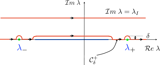
Figure 1: The integration contour ${\cal C}_{\delta}^{+}$

Let ${\cal C}_{\delta}^{-}$ be the contour deduced from ${\cal C}_{\delta}^{+}$ by symmetry with respect to the real axis (see Figure 2).

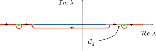
Figure 2: The integration contour ${\cal C}_{\delta^{-}}$

We claim that,

$$\int_{{\cal C}_{\delta}^{-}}\,{e^{-ik\lambda t}}\;\frac{N(\lambda)}{\big{(}\lambda-M(y)\big{)}^{\ell+1}}\;\,d\lambda=0.$$ (3.18)

This is obtained by considering the closed contour ${\cal C}_{R,\delta}^{-}$ of Figure 3 inside which the integrand is analytic.

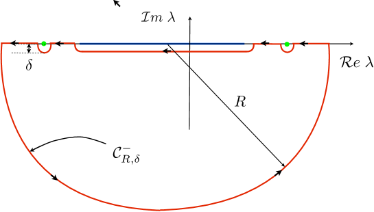
Figure 3: The integration contour ${\cal C}_{R,\delta}$

Thus, by Cauchy’s theorem

$$\int_{{\cal C}_{R,\delta}^{-}}\,{e^{-ik\lambda t}}\,\frac{N(\lambda)}{\big{(}\lambda-M(y)\big{)}^{\ell+1}}\;\;d\lambda=0.$$ (3.19)

Then, (3.18) is obtained from (3.19) by passing to the limit when $R\rightarrow+\infty$: the contribution of the integral along the semi-circle of radius $R$ vanishes because it is inside the good complex half-space when $k>0$ (for the exponential term) and because the function ${N(\lambda)}/{\big{(}\lambda-M(y)\big{)}^{\ell+1}}$ decays at infinity.
Finally adding (3.17) and (3.18), we obtain

$$I_{\ell}(kt,y)=\int_{{\cal C}_{\delta}}\,{e^{-ik\lambda t}}\;\frac{N(\lambda)}{\big{(}\lambda-M(y)\big{)}^{\ell+1}}\,d\lambda,$$ (3.20)

where ${\cal C}_{\delta}$ is the closed contour of Figure 4.

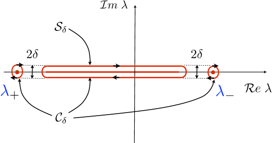
Figure 4: The integration contours ${\cal C}_{\delta}$ and ${\cal S}_{\delta}$

By the theorem of residues we also have:

$$I_{\ell}(kt,y)=I_{\ell,p}(kt,y)+I_{\ell,c}(kt,y),\quad\ell=1,2,$$ (3.21)

where

$$\left\{\begin{array}[]{l}\displaystyle\displaystyle I_{\ell,p}(kt,y):=-2i\pi\sum_{\pm}\;e^{-ik\lambda_{\pm}t}\,\frac{\mbox{Res}\,N(\lambda_{\pm})}{(\lambda_{\pm}-M(y))^{\ell+1}},\\[18.0pt] \displaystyle I_{\ell,c}(kt,y):=\int_{{\cal S}_{\delta}}\,{e^{-ik\lambda t}}\;\frac{N(\lambda)}{\big{(}\lambda-M(y)\big{)}^{\ell+1}}\;d\lambda,\end{array}\right.$$ (3.22)

where ${\cal S}_{\delta}$ is a closed curve that collapses to the segment $[M_{-},M_{+}]$ when $\delta$ goes to 0 (see Figure 4 again).

To get a more exploitable formula for $I_{\ell,c}(kt,y)$ , we would like to take the limit of the expression in the right-hand side when $\delta$ tends to 0. For this we need some additional information on the behaviour of $N(\lambda)$ when $\lambda$ approaches the segment $[M_{-},M_{+}]$. In the following we consider two different situations leading to quite different behaviours of $N(\lambda)$ when $\lambda$ approaches $[M_{-},M_{+}]$.

• The case of a class of smooth profiles with constant monotonicity and convexity (see Subsection 3.3.1). This is a physically relevant case for which $N(\lambda)$ has two distinct limits on $[M_{-},M_{+}]$ depending on whether one approaches the segment from above or from below. In this case, the function $N(\lambda)$ presents a cut along $[M_{-},M_{+}]$.

• The case (already considered in [3]) of a class of piecewise linear profiles (see Subsection 3.3.2), typically with fixed convexity . This case is interesting to provide a safe procedure for numerical approximations. In this situation, the function $N(\lambda)$ is meromorphic (it is a rational fraction) with real poles distributed in $[M_{-},M_{+}]$, as well as poles at $\lambda_{\pm}$.

3.3 Well-posedness results

3.3.1 For a class of smooth profiles

We denote by $C^{(n,\gamma)}[-1,1],n=0,1,\cdots,0<\gamma<1,$ the space of real-valued functions defined on $[-1,1]$ that are $n-$times differentiable and with the derivative of order $n$ Hölder continuous with exponent $\gamma$.

DEFINITION 3.2.

If $l$ denotes an integer $\geq 2$ and $\gamma$ a real number in $]0,1[$ , we shall say that a profile $M(y)$ belongs to the class ${\cal C}_{s}^{l,\gamma}$ if it fulfills the following conditions:

$$M\in C^{(l,\gamma)}[-1,1],\quad M^{\prime}(y)\neq 0,\quad M^{\prime\prime}(y)\neq 0,\quad\forall\;y\in[-1,1].$$ (3.23)

In other words, a profile in the class ${\cal C}_{s}^{l,\gamma}$ is smooth, strictly monotonous and has a fixed (strict) convexity.

LEMMA 3.3.

Suppose that $M(y)$ belongs to the class ${\cal C}_{s}^{l,\gamma}$ for some $l\geq 2$ and $\gamma\in]0,1[$. Then, it is stable in the sense that it satisfies the condition $({\cal H}_{S})$.

Proof: Without loss of generality, we can assume that $M$ is increasing (changing $M$ into $-M$ simply exchanges the signs of the roots of $F(\lambda)=2$) and that $M_{-}\big{(}\equiv M(-1)\big{)}=0$ (translating $M$ simply translates the solutions of $F(\lambda)=2$ parallel to the real axis). Since, by continuity, $M^{\prime}(y)$ is bounded from below by a strictly positive constant, we can write

$$F(\lambda)=\int_{-1}^{1}\frac{M^{\prime}(y)}{(M(y)-\lambda)^{2}}\;\frac{dy}{M^{\prime}(y)}=-\int_{-1}^{1}\frac{d}{dy}\left\{\frac{1}{(M(y)-\lambda)}\right\}\;\frac{dy}{M^{\prime}(y)}.$$

After integration by parts, we get

$$F(\lambda)=-\int_{-1}^{1}\frac{1}{(M(y)-\lambda)}\;\frac{M^{\prime\prime}(y)}{M^{\prime}(y)^{2}}\;dy-\Big{[}\frac{1}{(M(y)-\lambda)\,M^{\prime}(y)}\Big{]}_{-1}^{1}.$$

That is to say, for $\lambda=\lambda_{R}+i\lambda_{I}$,

$$\left|\begin{array}[]{l}\displaystyle{\cal R}e\;F(\lambda)=-\left\{\int_{-1}^{1}\frac{M(y)-\lambda_{R}}{|M(y)-\lambda|^{2}}\;\frac{M^{\prime\prime}(y)}{M^{\prime}(y)^{2}}\;dy+\Big{[}\frac{M(y)-\lambda_{R}}{|M(y)-\lambda)|^{2}\,M^{\prime}(y)}\Big{]}_{-1}^{1}\right\},\\[18.0pt] \displaystyle{\cal I}m\;F(\lambda)=-\lambda_{I}\left\{\int_{-1}^{1}\frac{1}{|M(y)-\lambda|^{2}}\;\frac{M^{\prime\prime}(y)}{M^{\prime}(y)^{2}}\;dy+\Big{[}\frac{1}{|M(y)-\lambda)|^{2}\,M^{\prime}(y)}\Big{]}_{-1}^{1}\right\}.\end{array}\right.$$

If $F(\lambda)=2$ with $\lambda_{I}\neq 0$, we have in particular

$$\int_{-1}^{1}\frac{1}{|M(y)-\lambda|^{2}}\;\frac{M^{\prime\prime}(y)}{M^{\prime}(y)^{2}}\;dy+\Big{[}\frac{1}{|M(y)-\lambda)|^{2}\,M^{\prime}(y)}\Big{]}_{-1}^{1}=0.$$ (3.24)

Substituting this in the right hand side of ${\cal R}e\;F(\lambda)$ (note that the above term is the multiplicative factor of $\lambda_{R}$), we get (since $M(-1)=0$ and setting $M^{\prime}_{\pm}=M^{\prime}(\pm 1)$ )

$${\cal R}e\;F(\lambda)=-\int_{-1}^{1}\frac{M(y)}{|M(y)-\lambda|^{2}}\;\frac{M^{\prime\prime}(y)}{M^{\prime}(y)^{2}}\;dy-\frac{M_{+}}{|M_{+}-\lambda|^{2}\,M^{\prime}_{+}}.$$

Next, we claim that ${\cal R}e\;F(\lambda)<0$ so that $,F(\lambda)=2$ is impossible. We distinguish two cases:

• $M^{\prime\prime}(y)>0$. In this case, ${\cal R}e\;F(\lambda)$ is clearly the sum of two negative terms.

• $M^{\prime\prime}(y)<0$. In this case, we can write

  $$\left|\begin{array}[]{ll}\displaystyle-\int_{-1}^{1}\frac{M(y)}{|M(y)-\lambda|^{2}}\;\frac{M^{\prime\prime}(y)}{M^{\prime}(y)^{2}}\;dy&\displaystyle\leq-\int_{-1}^{1}\frac{M_{+}}{|M(y)-\lambda|^{2}}\;\frac{M^{\prime\prime}(y)}{M^{\prime}(y)^{2}}\\[12.0pt] &\displaystyle=\Big{[}\frac{M_{+}}{|M(y)-\lambda)|^{2}\,M^{\prime}(y)}\Big{]}_{-1}^{1}.\end{array}\right.$$

  The second inequality being deduced from (3.24). Then,

  $${\cal R}e\;F(\lambda)\leq\Big{[}\frac{M_{+}}{|M(y)-\lambda)|^{2}\,M^{\prime}(y)}\Big{]}_{-1}^{1}-\frac{M_{+}}{|M_{+}-\lambda|^{2}\,M^{\prime}_{+}}=-\frac{M_{+}}{|\lambda|^{2}\,M^{\prime}_{-}}<0.$$

This achieves the proof.

$\Box$

Next, we wish to study $F(\lambda)$ when $\lambda$ approaches the segment $[M_{-},M_{+}]$, assuming that $M\in{\cal C}_{s}^{2}$. The idea is to use a well known result from the theory of Cauchy integrals (see [8], [9], and [10]). Let us first give some technical definitions.

DEFINITION 3.4.

Defining the complex open halfspaces as ${\mathbb{C}}^{\pm}=\{\lambda\in{\mathbb{C}}\,/\,\pm{\cal I}m\;\lambda>0\}$ we say that $h_{\pm}:\overline{{\mathbb{C}}^{\pm}}\longrightarrow{\mathbb{C}}$ is locally Hölder continuous in $\overline{{\mathbb{C}}^{\pm}}$ with exponent $\gamma\in\;]0,1[$ if

$$\forall\;R>0,\quad\exists\;C_{R}>0\quad/\quad\forall\;(\lambda_{1},\lambda_{2})\in{\cal B}_{R}^{\pm},\quad|h_{\pm}(\lambda_{1})-h_{\pm}(\lambda_{2})|\leq C_{R}\;|\lambda_{1}-\lambda_{2}|^{\gamma}$$ (3.25)

where ${\cal B}_{R}^{\pm}=\{\lambda\in\overline{{\mathbb{C}}^{\pm}}\,/\,|\lambda|\leq R$}. If the constant $C_{R}$ can be taken independent of $R$ we say that $h_{\pm}$ is Hölder continuous in $\overline{{\mathbb{C}}^{\pm}}$.
In the same way we say that $h_{\pm}:\overline{{\mathbb{C}}^{\pm}}\setminus\{M_{-},M_{+}\}\longrightarrow{\mathbb{C}}$ is locally Hölder continuous in $\overline{{\mathbb{C}}^{\pm}}\setminus\{M_{-},M_{+}\}$ with exponent $\gamma\in\;]0,1[$ if

$$\forall\;R,\delta>0,\quad\exists\;C_{R,\delta}>0\quad/\quad\forall\;(\lambda_{1},\lambda_{2})\in{\cal B}_{R,\delta}^{\pm},\quad|h_{\pm}(\lambda_{1})-h_{\pm}(\lambda_{2})|\leq C_{R,\delta}\,|\lambda_{1}-\lambda_{2}|^{\gamma}$$ (3.26)

where ${\cal B}_{R,\delta}^{\pm}=\{\lambda\in{\cal B}_{R}^{\pm}\,/\,|\lambda-M_{\pm}|\geq\delta\}$.

We quote below a classical result in Cauchy integrals that we use.

PROPOSITION 3.5.

(Plemelj-Privalov Theorem) Let $g(z):[M_{-},M_{+}]\rightarrow{\mathbb{C}}$ be Hölder continuous with exponent $\gamma\in\;]0,1[$ in $[M_{-},M_{+}]$. Define the function

$$S(\lambda)=\int_{M_{-}}^{M_{+}}\,\,g(z)\,(z-\lambda)^{-1}\,dz,\quad\lambda\in{\mathbb{C}}\setminus[M_{-},M_{+}].$$

Then, for any $\lambda\in{\mathbb{C}}\setminus]M_{-},M_{+}[$

$$\lim_{\varepsilon\downarrow 0}\,S(\lambda\pm i\varepsilon)=S_{\pm}(\lambda):=P.V.\,\int_{M_{-}}^{M_{+}}\,\,g(z)\,(z-\lambda)^{-1}\,dz\,\,\pm i\pi g(\lambda),$$ (3.27)

where $P.V.$ stands for the Cauchy principal value of the integral. The function

$$S_{\pm}(\lambda):=S(\lambda),\quad\mbox{if }\lambda\in\overline{{\mathbb{C}}^{\pm}}\setminus[M_{-},M_{+}]\quad\mbox{and}\quad S_{\pm}(\lambda),\quad\mbox{if }\lambda\in\;]M_{-},M_{+}[,$$ (3.28)

is analytic in ${\mathbb{C}}^{\pm}$ and locally Hölder continuous with exponent $\gamma$ in $\overline{{\mathbb{C}}^{\pm}}\setminus\{M_{-},M_{+}\}$. Moreover, if $g(M_{+})=g(M_{-})=0$ , $S_{\pm}(\lambda)$ can be continuously extended to $\overline{{\mathbb{C}}^{\pm}}$ into a function which is locally Hölder continuous in $\overline{{\mathbb{C}}^{\pm}}$. Conversely, if $g(M_{\pm})\neq 0$, $S_{\pm}(\lambda)$ blows up as a logarithm when $\lambda$ tends to $M_{\pm}$.

In what follows, we assume that $M\in{\cal C}^{3,\gamma}_{s}$. For the sequel, it will be useful to introduce $\mu(z)$ the inverse function to $M(y)$,

$$\mu(z)=y,\quad\hbox{\rm for}\,z=M(y),\quad y\in[-1,1].$$ (3.29)

Changing the variable of integration to $z=M(y)$, we have that,

$$F(\lambda)=\int_{M_{-}}^{M_{+}}\,\mu^{\prime}(z)\,(z-\lambda)^{-2}\,dz,\quad\lambda\in{\mathbb{C}}\setminus[M_{-},M_{+}].$$ (3.30)

In order to apply Proposition 3.5, we integrate by parts in (3.30) and obtain that,

$$F(\lambda)=-\mu^{\prime}(z)\,(z-\lambda)^{-1}\Big{|}^{M_{+}}_{M_{-}}+\int_{M_{-}}^{M_{+}}\,\mu^{\prime\prime}(z)\,(z-\lambda)^{-1}\,dz.$$ (3.31)

Applying Proposition 3.5 with $g=\mu^{\prime\prime}$, we get

$$\left\{\begin{array}[]{l}\lim_{\varepsilon\downarrow 0}\,F(\lambda\pm i\varepsilon)=F_{\pm}(\lambda),\quad\forall\;\lambda\in]M_{-},M_{+}[,\\[12.0pt] \displaystyle F_{\pm}(\lambda):=-\mu^{\prime}(z)\,(z-\lambda)^{-1}\Big{|}^{M_{+}}_{M_{-}}+P.V.\,\int_{M_{-}}^{M_{+}}\,\,\mu^{\prime\prime}(z)\,(z-\lambda)^{-1}\,dz\,\,\pm i\pi\mu^{\prime\prime}(\lambda),\end{array}\right.$$ (3.32)

and we can define as in Proposition 3.5, formula (3.28), $F_{\pm}(\lambda)$ as a function that is analytic in ${\mathbb{C}}^{\pm}$ and locally Hölder continuous with exponent $\gamma$ in $\overline{{\mathbb{C}}^{\pm}}\setminus\{M_{-},M_{+}\}$. Note that for $\lambda\in\;]M_{-},M_{+}[,{\cal I}m\;F_{\pm}(\lambda)=\pm\pi\,\mu^{\prime\prime}(\lambda)\neq 0$, in particular $F_{\pm}(\lambda)-2\neq 0$, which allows us to state the following result.

LEMMA 3.6.

Assume that $M\in{\cal C}^{2,\gamma}_{s}$. Then, for any $\lambda\in\;]M_{-},M_{+}[$

$$\lim_{\varepsilon\downarrow 0}\,N(\lambda\pm i\varepsilon)=\big{(}2-F_{\pm}(\lambda)\big{)}^{-1}.$$ (3.33)

Moreover, the function

$$N_{\pm}(\lambda):=\left\{\begin{array}[]{ll}N(\lambda),&\lambda\in{\mathbb{C}}^{\pm}=\{z\in{\mathbb{C}}\,/\,\pm{\cal I}m\,z>0\},\\ \\ \big{(}F_{\pm}(\lambda)-2\big{)}^{-1},&\lambda\in\;]M_{-},M_{+}[,\end{array}\right.$$ (3.34)

is extended by continuity to $\overline{{\mathbb{C}}^{\pm}}$, with $N_{\pm}(M)=0$ for $M=M_{+}$ or $M_{-}$, as a function analytic in ${\mathbb{C}}^{\pm}$ and Hölder continuous in $\overline{{\mathbb{C}}^{\pm}}$ with exponent $\gamma$. Moreover,

$$\begin{array}[]{l}\forall\;\lambda\in[M_{-},M_{+}],\quad N_{-}(\lambda)=\overline{N_{+}(\lambda)},\quad\mbox{i. e. }N_{\pm}(\lambda)={\cal R}e\;N(\lambda)\pm i\,{\cal I}m\;N(\lambda),\end{array}$$ (3.35)

where ${\cal R}e\;N$ is the common value of ${\cal}Re\;N_{+}$ and ${\cal R}e\;N_{-}$ and ${\cal I}m\;N:={\cal I}m\;N_{+}=-{\cal I}m\;N_{-}$.

REMARK 3.7.

One can easily obtain an explicit expression of ${\cal R}e\;N$ and ${\cal I}m\;N$ from (3.32) and (3.28). For instance, one has

$${\cal I}m\;N(\lambda)=\pi\,|N_{\pm}(\lambda)|^{2}\;\mu^{\prime\prime}(\lambda),\quad\lambda\in[M_{-},M_{+}].$$ (3.36)

Such expressions are, in particular, useful for numerical computations (see [6]).

Proof: The continuous extension by $N_{\pm}(M_{\pm})=0$ is valid by (3.31). The local Hölder continuity of $N_{\pm}$ in $\overline{{\mathbb{C}}^{\pm}}\setminus\{M_{-},M_{+}\}$ is inherited from the same property for $F_{\pm}$. The Hölder continuity up to $M_{\pm}$ remains to be clarified. We consider the case of $M_{+}$ ($M_{-}$ is treated analogously) and introduce the function

$$J^{+}(\lambda)=(M_{+}-\lambda)\,\big{(}2-F_{\pm}(\lambda)\big{)},\quad\mbox{ such that }N_{\pm}(\lambda)=(M_{+}-\lambda)\,J^{+}(\lambda)^{-1}.$$

We can conclude if we show that $J^{+}$ is Hölder continuous in a neighborhood of $M_{+}$ and does not vanish at $M=M_{+}$. According to (3.31),

$$J^{+}(\lambda)=\mu^{\prime}(M_{+})+{(M_{+}-\lambda)}\;\Big{(}2-\frac{\mu^{\prime}(M_{-})}{M_{-}-\lambda}-\int_{M_{-}}^{M_{+}}\,\,\frac{\mu^{\prime\prime}(z)}{z-\lambda}\,dz\Big{)},$$

that we rewrite as

$$\left|\begin{array}[]{lll}J^{+}(\lambda)=\mu^{\prime}(M_{+})&+&\displaystyle{(M_{+}-\lambda)}\;\Big{(}2-\frac{\mu^{\prime}(M_{-})}{M_{-}-\lambda}-\mu^{\prime\prime}(M_{+})\log\left[\frac{M_{+}-\lambda}{M_{-}-\lambda}\right]\Big{)}\\[12.0pt] &-&\displaystyle{(M_{+}-\lambda)}\;\int_{M_{-}}^{M_{+}}\,\,\frac{\mu^{\prime\prime}(z)-\mu^{\prime\prime}(M_{+})}{z-\lambda}\,dz.\end{array}\right.$$ (3.37)

Consequently, since

• $x\mapsto x\,\log x$ is Hölder continuous with any exponent in $(0,1)$,

• by Proposition 3.5 applied with $g(z)=\mu^{\prime\prime}(z)-\mu^{\prime\prime}(M_{+})$ (that satisfies $g(M_{+})=0$),

  $$\lambda\rightarrow\int_{M_{-}}^{M_{+}}\,\,\frac{\mu^{\prime\prime}(z)-\mu^{\prime\prime}(M_{+})}{z-\lambda}\,dz\quad\mbox{ is H\"{o}lder continuous with exponent }\gamma,$$

we deduce from (3.37) that $J_{+}$ is Hölder continuous with exponent $\gamma$ in a neighborhood of $M_{+}$. Finally, $J^{+}(M_{+})=\mu^{\prime}(M_{+})\neq 0$, since $M\in{\cal C}^{2,\gamma}_{s}$.

$\Box$
We shall need an analogous result for $N^{\prime}(\lambda)$, the derivative of $N(\lambda)$. For this, we assume that $M\in{\cal C}^{3,\gamma}_{s}$ and remark that for $\lambda\in{\mathbb{C}}\setminus[M_{-},M_{+}]$

$$\left|\begin{array}[]{lll}F^{\prime}(\lambda)&=&\displaystyle-\int_{M_{-}}^{M_{+}}\,\mu^{\prime}(z)\,\frac{d}{dz}\left[(z-\lambda)^{-2}\right]\,dz\\[12.0pt] &=&\displaystyle-\mu^{\prime}(z)\,(z-\lambda)^{-2}\Big{|}^{M_{+}}_{M_{-}}+\int_{M_{-}}^{M_{+}}\,\mu^{\prime\prime}(z)\,(z-\lambda)^{-2}\,dz.\\[12.0pt] &=&\displaystyle-\mu^{\prime}(z)\,(z-\lambda)^{-2}\Big{|}^{M_{+}}_{M_{-}}-\mu^{\prime\prime}(z)\,(z-\lambda)^{-1}\Big{|}^{M_{+}}_{M_{-}}+\int_{M_{-}}^{M_{+}}\,\mu^{\prime\prime\prime}(z)\,(z-\lambda)^{-1}\,dz.\end{array}\right.$$ (3.38)

Applying Proposition 3.5 as for $F(\lambda)$, we obtain

$$\left\{\begin{array}[]{l}\lim_{\varepsilon\downarrow 0}\,F^{\prime}(\lambda\pm i\varepsilon)=F^{\prime}_{\pm}(\lambda),\quad\forall\;\lambda\in]M_{-},M_{+}[,\\[12.0pt] \begin{array}[]{lll}\displaystyle F^{\prime}_{\pm}(\lambda)&:=&-\mu^{\prime}(z)\,(z-\lambda)^{-2}\Big{|}^{M_{+}}_{M_{-}}-\mu^{\prime\prime}(z)\,(z-\lambda)^{-1}\Big{|}^{M_{+}}_{M_{-}}\\[12.0pt] &+&\displaystyle P.V.\,\int_{M_{-}}^{M_{+}}\,\,\mu^{\prime\prime\prime}(z)\,(z-\lambda)^{-1}\,dz\,\,\pm i\pi\mu^{\prime\prime\prime}(\lambda),\end{array}\end{array}\right.$$ (3.39)

and we can define again as in Proposition 3.5, formula (3.28), $F^{\prime}_{\pm}(\lambda)$ as a function that is analytic in ${\mathbb{C}}^{\pm}$ and locally Hölder continuous with exponent $\gamma$ in $\overline{{\mathbb{C}}^{\pm}}\setminus\{M_{-},M_{+}\}$. Next we state for $N^{\prime}$ the equivalent result of Lemma 3.3 for $N$.

LEMMA 3.8.

Assume that $M\in{\cal C}^{3,\gamma}_{s}$. Then, for any $\lambda\in\;]M_{-},M_{+}[$

$$\lim_{\varepsilon\downarrow 0}\,N^{\prime}(\lambda\pm i\varepsilon)=-F^{\prime}_{\pm}(\lambda)\;\big{(}2-F_{\pm}(\lambda)\big{)}^{-2}.$$ (3.40)

Moreover, the function

$$N^{\prime}_{\pm}(\lambda):=\left\{\begin{array}[]{ll}N^{\prime}(\lambda),&\lambda\in{\mathbb{C}}^{\pm}=\{z\in{\mathbb{C}}\,/\,\pm{\cal I}m\;z>0\},\\ \\ -F^{\prime}_{\pm}(\lambda)\;\big{(}2-F_{\pm}(\lambda)\big{)}^{-2},&\lambda\in\;]M_{-},M_{+}[,\end{array}\right.$$ (3.41)

is extended by continuity to $\overline{{\mathbb{C}}^{\pm}}$ with

$$N^{\prime}_{\pm}(M)=-\frac{\mu^{\prime\prime}(M)}{\mu^{\prime}(M)^{2}}\quad\mbox{for }M=M_{+}\mbox{ or }M_{-}.$$ (3.42)

Then, $N^{\prime}_{\pm}(\lambda)$ is analytic in ${\mathbb{C}}^{\pm}$ and Hölder continuous in $\overline{{\mathbb{C}}^{\pm}}$ with exponent $\gamma$. Moreover,

$$\begin{array}[]{l}\forall\;\lambda\in[M_{-},M_{+}],\quad N^{\prime}_{-}(\lambda)=\overline{N^{\prime}_{+}(\lambda)},\quad\mbox{i. e. }N^{\prime}_{\pm}(\lambda)={\cal R}e\;N^{\prime}(\lambda)\pm\,i\,{\cal I}m\;N^{\prime}(\lambda),\end{array}$$ (3.43)

where ${\cal R}e\;N^{\prime}$ is the common value of ${\cal R}e\;N^{\prime}_{+}$ and ${\cal R}e\;N^{\prime}_{-}$ and ${\cal I}m\;N^{\prime}={\cal I}m\;N^{\prime}_{+}=-{\cal I}m\;N^{\prime}_{-}$.

Proof: It is very similar to the proof of Lemma 3.3. From formula (3.38), using the same trick used for proving the Hölder continuity of $J^{+}(\lambda)$ (see the proof of Lemma 3.3), we deduce that:

$$F^{\prime}_{\pm}(\lambda)=(M_{+}-\lambda)^{-2}\big{[}\,-\mu^{\prime\prime}(M_{+})+h(\lambda)\big{]},\quad h\in{\cal C}^{0,\gamma},\quad h(0)=0.$$

Therefore, since $N_{\pm}(\lambda)^{2}=(M_{+}-\lambda)^{2}\;J^{+}(\lambda)^{-2}$,

$$N^{\prime}_{\pm}(\lambda)=-F^{\prime}_{\pm}(\lambda)\;N_{\pm}(\lambda)^{2}=\big{[}\,-\mu^{\prime\prime}(M_{+})+h(\lambda)\big{]}\;J^{+}(\lambda)^{-2}.$$

It is then easy to conclude.

$\Box$

REMARK 3.9.

Again we can easily obtain an explicit expression of ${\cal R}e\;N^{\prime}$ and ${\cal I}m\;N^{\prime}$ from (3.39) and (3.34) (see [6]).

With Lemmata 3.3 and 3.8, we now have all the needed information for studying the integrals $I_{\ell}(kt,y),\ell=0,1$. We first obtain a new expression for $I_{\ell,c}(kt,y)$:

LEMMA 3.10.

Assume that $M\in{\cal C}^{2,\gamma}_{s}$, then

$$\left|\begin{array}[]{lll}I_{0,c}(kt,y)&:=&\displaystyle P.V.\int_{M_{-}}^{M_{+}}\,{e^{-ik\lambda t}}\;\frac{\big{[}\,N_{+}(\lambda)-N_{-}(\lambda)\big{]}}{\big{(}\lambda-M(y)\big{)}}\;d\lambda\\[18.0pt] &-&\displaystyle i\pi\big{[}\,N_{+}\big{(}M(y)\big{)}+N_{-}\big{(}M(y)\big{)}\,\big{]}\;{e^{-ikM(y)t}}.\end{array}\right.$$ (3.44)

If moreover, $M\in{\cal C}^{3,\gamma}_{s}$, then

$$\left|\begin{array}[]{lll}\displaystyle I_{1,c}(kt,y)&:=&\displaystyle-ikt\;I_{0,c}(kt,y)+P.V.\int_{M_{-}}^{M_{+}}\,{e^{-ik\lambda t}}\;\frac{\big{[}\,N^{\prime}_{+}(\lambda)-N^{\prime}_{-}(\lambda)\,\big{]}}{\big{(}\lambda-M(y)\big{)}}\;d\lambda\\[18.0pt] &-&\displaystyle i\pi\big{[}\,N^{\prime}_{+}\big{(}M(y)\big{)}+N^{\prime}_{-}\big{(}M(y)\big{)}\,\big{]}\;{e^{-ikM(y)t}}.\end{array}\right.$$ (3.45)

Proof: Let us start from the formula (3.22) for $I_{0,c}(kt,y)$ that we can rewrite:

$$I_{0,c}(kt,y):=\sum_{\pm}\int_{\gamma_{\delta}^{\pm}}\;\frac{N_{\pm,kt}(\lambda)}{\big{(}\lambda-M(y)\big{)}}\;d\lambda+\sum_{\pm}(\pm 1)\cdot\int_{M_{-}}^{M_{+}}\;\frac{N_{kt}(\lambda\pm i\delta)}{\big{(}\lambda\pm i\delta-M(y)\big{)}}\;d\lambda$$

where $N_{\pm,kt}(\lambda):=N_{\pm}(\lambda)\;e^{-ikt\lambda}$. Since $N(M_{\pm})=0$,

$$\lim_{\delta\rightarrow 0}\int_{\gamma_{\delta}^{\pm}}\;\frac{N_{kt}(\lambda)}{\big{(}\lambda-M(y)\big{)}}\;d\lambda=0,$$

so that

$$I_{0,c}(kt,y)=\lim_{\delta\rightarrow 0}\int_{M_{-}}^{M_{+}}\;\frac{N_{+,kt}(\lambda+i\delta)}{\big{(}\lambda+i\delta-M(y)\big{)}}\;d\lambda-\lim_{\delta\rightarrow 0}\int_{M_{-}}^{M_{+}}\;\frac{N_{-,kt}(\lambda-i\delta)}{\big{(}\lambda-i\delta-M(y)\big{)}}\;d\lambda,$$

that we rewrite as

$$I_{0,c}(kt,y)=\Big{[}\,I_{0,c}^{(1,+)}(kt,y)-I_{0,c}^{(1,-)}(kt,y)\,\Big{]}+\Big{[}\,I_{0,c}^{(2,+)}(kt,y)-I_{0,c}^{(2,-)}(kt,y)\,\Big{]},$$

where

$$\left|\begin{array}[]{l}\displaystyle I_{0,c}^{(1,\pm)}(kt,y)=\lim_{\delta\rightarrow 0}\int_{M_{-}}^{M_{+}}\;\frac{N_{\pm,kt}(\lambda\pm i\delta)-N_{\pm,kt}(\lambda)}{\big{(}\lambda\pm i\delta-M(y)\big{)}},\\[18.0pt] \displaystyle I_{0,c}^{(2,\pm)}(kt,y)=\lim_{\delta\rightarrow 0}\int_{M_{-}}^{M_{+}}\;\frac{N_{\pm,kt}(\lambda)}{\big{(}\lambda\pm i\delta-M(y)\big{)}}.\end{array}\right.$$

The Hölder continuity of $N_{\pm,kt}(\lambda)$ (see Lemma 3.3) implies $I_{0,c}^{(1,\pm)}(kt,y)=0$. Then, it is sufficient to apply again Proposition 3.5 with $g=-N(\lambda)\,e^{-ikt}$ to get the result.
For $I_{1,c}(kt,y)$, we first integrate by parts in (3.22) to obtain

$$I_{1,c}(kt,y):=\int_{{\cal S}_{\delta}}\,\;\frac{N_{kt}^{\prime}(\lambda)}{\big{(}\lambda-M(y)\big{)}}\;d\lambda.$$

We then proceed as above using $N_{\pm,kt}^{\prime}(\lambda)=\big{(}N_{\pm}^{\prime}(\lambda)-iktN_{\pm}(\lambda)\big{)}\;e^{-ikt\lambda}$ and Lemma 3.8. The details are left to the reader.

$\Box$
We are now in position to derive our estimates for $I_{\ell}(kt,y),\ell=0,1$.

LEMMA 3.11.

Assume that $M\in{\cal C}^{\ell+1}_{s},\ell=1,2$. Then, there exists a constant $I_{\ell}^{*}>0$, depending only on $\ell$ and $M$, such that one has the uniform estimates:

$$\forall\;k\in{\mathbb{R}},\quad\forall\;t>0,\quad\|I_{\ell}(kt,\cdot)\|_{L^{\infty}([-1,1])}\leq I_{\ell}^{*}\;(1+\ell\;|kt|^{\ell}),\quad\ell=0,1.$$ (3.46)

Proof: Remarking that, thanks to (3.35), $(N_{+}+N_{-})(\lambda)=2{\cal R}e\;N(\lambda)$ and setting

$$\Delta N(\lambda):=(N_{+}-N_{-})(\lambda)=2i({\cal I}m\;N(\lambda)\equiv 2\,i\,\pi\,|N_{\pm}(\lambda)|^{2}\mu^{\prime\prime}(\lambda),$$ (3.47)

by (3.35) and (3.36). From (3.44) we deduce that,

$$I_{0,c}(kt,y)\leq|\,P.V.\int_{M_{-}}^{M_{+}}\,{e^{-ik\lambda t}}\;\frac{\Delta N(\lambda)}{\big{(}\lambda-M(y)\big{)}}\;d\lambda\,|+2\pi\;{\cal R}e\;N\big{(}M(y)\big{)}|.$$ (3.48)

By Lemma 3.3 we know that $\Delta N(\lambda)$ is Hölder continuous with exponent $\gamma$. Since $\Delta N(\lambda)=0$, for $\lambda\leq M_{-}$ and for $\lambda\geq M_{+}$, we can write, denoting $L=M_{+}-M_{-}$ (so that $M(y)-L\leq M_{-}$ and $M(y)+L\geq M_{+}$),

$$\left|\begin{array}[]{ll}\displaystyle P.V.\int_{M_{-}}^{M_{+}}\,{e^{-ik\lambda t}}\;\frac{\Delta N(\lambda)}{\big{(}\lambda-M(y)\big{)}}\;d\lambda\displaystyle=P.V.\int_{M(y)-L}^{M(y)+L}\,{e^{-ik\lambda t}}\;\frac{\Delta N(\lambda)}{\big{(}\lambda-M(y)\big{)}}\;d\lambda\\[18.0pt] \quad\quad\quad\quad\quad\quad\quad\quad\displaystyle=\;e^{-ikM(y)t}\;P.V.\int_{-L}^{L}\,{e^{-ik\nu t}}\;\frac{\Delta N\big{(}\nu+M(y)\big{)}}{\nu}\;d\nu.\end{array}\right.$$ (3.49)

Next, we write

$$\left|\begin{array}[]{ll}\displaystyle P.V.\int_{-L}^{L}\,{e^{-ik\nu t}}\;\frac{\Delta N\big{(}\nu+M(y)\big{)}}{\nu}\;d\nu&\displaystyle=\int_{-L}^{L}\,{e^{-ik\nu t}}\;\frac{\Delta N\big{(}\nu+M(y)\big{)}-\Delta N\big{(}M(y)\big{)}}{\nu}\;d\nu\\[18.0pt] &\displaystyle+\;{\Delta N}\big{(}M(y)\big{)}\;\Big{(}P.V.\int_{-L}^{L}\,\frac{e^{-ik\nu t}}{\nu}\;d\nu\Big{)}.\end{array}\right.$$ (3.50)

Finally, we remark that

$$P.V.\int_{-L}^{L}\,\frac{e^{-ik\nu t}}{\nu}\;d\nu=-i\int_{-L}^{L}\,\frac{\sin({k\nu t})}{\nu}\;d\nu=-i\int_{-Lkt}^{Lkt}\,\frac{\sin(\xi)}{\xi}\;d\xi$$

is bounded (in modulus) since

$$\Big{|}\int_{-\infty}^{+\infty}\,\frac{\sin(\xi)}{\xi}\;d\xi\Big{|}=\lim_{A\rightarrow+\infty}\Big{|}\int_{-A}^{A}\,\frac{\sin(\xi)}{\xi}\;d\xi\Big{|}<+\infty.$$

Finally, if we set

$$K:=\sup_{A>0}\Big{|}\int_{-A}^{A}\,\frac{\sin(\xi)}{\xi}\;d\xi\Big{|}\quad\mbox{and}\quad|\Delta{N}|_{\gamma}:=\sup_{(x,y)\in{\mathbb{R}}^{2}}\frac{|\Delta N(x)-\Delta N(y)|}{|x-y|^{\gamma}}\;,$$ (3.51)

we deduce from (3.49) and (3.50) that ($\|\cdot\|_{L^{\infty}}$ meaning $\|\cdot\|_{L^{\infty}(-M_{-},M_{+})}$):

$$\Big{|}P.V.\int_{-L}^{L}\,{e^{-ik\nu t}}\;\frac{\Delta N\big{(}\nu+M(y)\big{)}}{\nu}\;d\nu\Big{|}\displaystyle\leq\Big{(}\int_{-L}^{L}\frac{d\nu}{|\nu|^{1-\gamma}}\Big{)}\;|\Delta N|_{\gamma}+K\;\|\Delta{N}\|_{L^{\infty}},$$ (3.52)

which, using (3.48), gives:

$$|I_{0,c}(kt,y)|\leq I_{0,c}^{*}:=2\,\frac{|M_{+}-M_{-}|^{\gamma}}{\gamma}\;|\Delta{N}|_{\gamma}+K\;\|\Delta{N}\|_{L^{\infty}}+2\pi\|\Re N\|_{L^{\infty}}.$$ (3.53)

Finally, since (see (3.21, 3.22)),

$$|I_{0}(kt,y)|\leq 2\pi\sum_{\pm}\frac{|\mbox{Res}\,N(\lambda_{\pm})|}{|\lambda_{\pm}-M(y)|}+|I_{0,c}(kt,y)|$$

we obtain the inequality (3.46) for $\ell=0$ with

$$I_{0}^{*}=I_{0,c}^{*}+2\pi\sum_{\pm}|\mbox{Res}\,N(\lambda_{\pm})|\;\|\frac{1}{\lambda_{\pm}-M(\cdot)}\|_{L^{\infty}}.$$

The inequality (3.46) for $\ell=1$ is derived analogously using (3.45) and Lemma 3.8. This time, instead of $\Delta N$, we have to work with $\Delta N^{\prime}:=N_{+}^{\prime}-N_{-}^{\prime}$ which fortunately satisfies $\Delta N^{\prime}(\lambda)=0$ for $\lambda\in(-\infty,M_{-}]\cup[M_{+},\infty)$, thanks to (3.42). Note that the additional factor $|kt|$ comes from the first term in the right-hand side of (3.45).

$\Box$
We now go back to the estimates of $\hat{\bf a}_{0}$ and $\hat{\bf a}_{1}$. Using the fact that $\displaystyle|{\bf a}(uv)|\leq\|u\|_{L^{2}_{y}}\,\|v\|_{L^{2}_{y}}$ (Cauchy-Schwartz) and $\|u\|_{L^{2}_{y}}\leq\sqrt{2}\,\|u\|_{L^{\infty}_{y}}$, we deduce from (3.13) and Lemma 3.11 that for $n=0,1,\cdots$,

$$|k|^{1+n}\;|\hat{\bf a}_{0}(k,t)|\leq\frac{\sqrt{2}}{\pi}\;\Big{(}I_{0}^{*}+I_{1}^{*}\;\|M\|_{L^{\infty}}\big{(}1+|kt|\big{)}\Big{)}\;|k|^{1+n}\;\|\hat{u}^{0}(k,\cdot)\|_{L^{2}_{y}}.$$ (3.54)

In the same way, from (3.14) and again Lemma 3.11, we obtain

$$|k|^{1+n}\;|\hat{\bf a}_{1}(k,t)|\leq\frac{\sqrt{2}}{\pi}\;I_{1}^{*}\;\big{(}1+|kt|\big{)}\;|k|^{n}\;\|\hat{u}^{1}(k,\cdot)\|_{L^{2}_{y}},\quad n=0,1,\cdots.$$ (3.55)

Thus, by Plancherel’s theorem, we see that, $C$ denoting a constant depending on $\|M\|_{L^{\infty}},I_{0}^{*}$ and $I_{1}^{*}$ (and thus on $M$ only),

$$\left|\begin{array}[]{ll}\displaystyle\|\frac{\partial^{1+n}{\bf a}(u)}{\partial x^{1+n}}(\cdot,t)\|_{L^{2}_{x}}\;\leq\;C&\displaystyle\Big{(}\;\|\frac{\partial^{1+n}u^{0}}{\partial x^{1+n}}\|_{L^{2}_{y}(L^{2}_{x})}+\|\frac{\partial^{n}u^{1}}{\partial x^{n}}\|_{L^{2}_{y}(L^{2}_{x})}\\[12.0pt] &\;\;\;\displaystyle+\;\;t\;\Big{[}\,\|\frac{\partial^{2+n}u^{0}}{\partial x^{2+n}}\|_{L^{2}_{y}(L^{2}_{x})}+\|\frac{\partial^{1+n}u^{1}}{\partial x^{1+n}}\|_{L^{2}_{y}(L^{2}_{x})}\,\Big{]}\;\Big{)},\end{array}\right.$$ (3.56)

for $n=0,1,\cdots$.

From (3.1), or equivalently (3.3), one easily deduces that for each $y\in]-1,1[$ and $t\geq 0$:

$$\begin{array}[]{l}\displaystyle u(x,y,t)=u^{0}(x-tM(y),y)+t\left(u^{1}(x-M(y)t,y)+M(y)\frac{\partial}{\partial x}u^{0}(x-M(y)t,y)\right)\\ \\ \hskip 42.67912pt+\int_{0}^{t}\,dz_{1}\,\int_{0}^{z_{1}}\,dz_{2}\,\frac{\partial^{2}{\bf a}(u)}{\partial x^{2}}(x-tM(y)+z_{2}M(y),z_{2}),\end{array}$$ (3.57)

for all $t>0,(x,y)\in{\mathbb{R}}\times[-1,1]$. Taking the $L^{2}$-norm in $y$ and using (3.56), we easily obtain (with another constant $C$ depending only on $M$)

$$\left|\begin{array}[]{l}\displaystyle\|\frac{\partial^{n}u(x,y,t)}{\partial x^{n}}\|_{L^{2}_{y}(L^{2}_{x})}\;\leq\displaystyle\|\frac{\partial^{n}u^{0}}{\partial x^{n}}(\cdot,y)\|_{L^{2}_{y}(L^{2}_{x})}+\displaystyle t\;\Big{(}\;\|\frac{\partial^{n}u^{1}(\cdot,y)}{\partial x^{n}}\|_{L^{2}_{y}(L^{2}_{x})}+\\[12.0pt] \displaystyle\|M\|_{L^{\infty}}\;\|\frac{\partial^{1+n}u^{0}}{\partial x^{1+n}}(\cdot,y)\|_{L^{2}_{y}(L^{2}_{x})}\;\Big{)}\displaystyle+C\;\displaystyle t^{2}\;\Big{(}\,\|\frac{\partial^{2+n}u^{0}}{\partial x^{2+n}}\|_{L^{2}_{y}(L^{2}_{x})}+\|\frac{\partial^{1+n}u^{1}}{\partial x^{1+n}}\|_{L^{2}_{y}(L^{2}_{x})}\,\Big{)}\\[12.0pt] \displaystyle+\displaystyle C\;t^{3}\;\Big{(}\,\|\frac{\partial^{3+n}u^{0}}{\partial x^{3+n}}\|_{L^{2}_{y}(L^{2}_{x})}+\|\frac{\partial^{2+n}u_{1}}{\partial x^{2+n}}\|_{L^{2}_{y}(L^{2}_{x})}\,\Big{)},\quad n=0,1,\cdots.\end{array}\right.$$ (3.58)

Concerning $\displaystyle\frac{\partial u}{\partial t}$ we observe that taking the time derivative amounts to the following: in the first equation in (3.22) to multiplication by $-ik\lambda_{\pm}$, and in equations (3.44, 3.45) to multiplication by $-ik\lambda,\lambda\in[M_{-},M_{+}]$ and by $-ikM(y)$. We easily see that arguing as above one obtains estimates for $\displaystyle|\frac{\partial\hat{\bf a}_{0}}{\partial t}(k,t)|$ and for $\displaystyle|\frac{\partial\hat{\bf a}_{1}}{\partial t}(k,t)|$ which are similar to those for $\displaystyle|\hat{\bf a}_{0}(k,t)|$ and $\displaystyle|\hat{\bf a}_{1}(k,t)|$ up to an extra power of $|k|$. As a consequence, it is easy to obtain the following estimate for the mean value of ${\bf a}(u)$:

$$\left|\begin{array}[]{l}\displaystyle\|\frac{\partial^{1+n}{\bf a}(u)}{\partial t\partial x^{n}}(x,t)\|_{L^{2}_{x}}\;\leq\;C\displaystyle\Big{(}\;\|\frac{\partial^{1+n}u^{0}}{\partial x^{1+n}}\|_{L^{2}_{y}(L^{2}_{x})}+\|\frac{\partial^{n}u^{1}}{\partial x^{n}}\|_{L^{2}_{y}(L^{2}_{x})}\;\;\;\displaystyle+\\[12.0pt] t\Big{[}\,\|\frac{\partial^{2+n}u^{0}}{\partial x^{2+n}}\|_{L^{2}_{y}(L^{2}_{x})}+\|\frac{\partial^{1+n}u^{1}}{\partial x^{1+n}}\|_{L^{2}_{y}(L^{2}_{x})}\,\Big{]}\;\Big{)},\quad n=0,1,\cdots.\end{array}\right.$$ (3.59)

Furthermore, taking the time derivative in both sides of (3.57), we obtain that,

$$\left|\begin{array}[]{l}\displaystyle\|\frac{\partial^{1+n}u}{\partial t\partial x^{n}}(x,y,t)\|_{L^{2}_{y}(L^{2}_{x})}\;\leq\displaystyle\|(1+M(y))\frac{\partial^{n+1}u^{0}}{\partial x^{n+1}}\|_{L^{2}_{y}(L^{2}_{x})}+\|\frac{\partial^{n}u^{1}}{\partial x^{n}}\|_{L^{2}_{y}(L^{2}_{x})}+\\[12.0pt] Ct\;\Big{(}\;\|\frac{\partial^{2+n}u^{0}}{\partial x^{2+n}}\|_{L^{2}_{y}(L^{2}_{x})}+\|\frac{\partial^{n+1}u^{1}}{\partial x^{n+1}}\|_{L^{2}_{y}(L^{2}_{x})}\Big{)}+\displaystyle C\;t^{2}\;\Big{(}\,\|\frac{\partial^{3+n}u^{0}}{\partial x^{3+n}}\|_{L^{2}_{y}(L^{2}_{x})}+\|\frac{\partial^{2+n}u^{1}}{\partial x^{2+n}}\|_{L^{2}_{y}(L^{2}_{x})}\,\Big{)}\\[12.0pt] Ct^{3}\Big{(}\,\|\frac{\partial^{4+n}u^{0}}{\partial x^{4+n}}\|_{L^{2}_{y}(L^{2}_{x})}+\,\|\frac{\partial^{3+n}u^{1}}{\partial x^{3+n}}\|_{L^{2}_{y}(L^{2}_{x})}\Big{)},\quad n=0,1,\cdots.\end{array}\right.$$ (3.60)

In the proof of estimates (3.58, 3.59, 3.60) we were not bothered by factor $1/k$ in the right-hand side of equation (3.14) because we only needed to estimate $\frac{\partial^{1+n}{\bf a}(u)}{\partial x^{2}}$ what implies that we have to multiply $\hat{\bf a}(u)$ by $(ik)^{1+n}$, what removes the singularity at $k=0$. However, as ${\bf a}(u)$ is a relevant physical variable it is important to estimate it directly. To do this we proceed below in a slightly different way. We define,

$$I(k,t,y):=\frac{1}{2\pi k}I_{1}(kt,y).$$ (3.61)

Then, equation (3.14) is replaced by,

$$\hat{\bf a}_{1}(k,t)=-2{\bf a}\Big{(}I(k,t,\cdot)\,\hat{u}^{1}(k,\cdot)\Big{)}.$$ (3.62)

We regularize the singularity at $k=0$ in $I$ as follows. By Cauchy’s theorem,

$$\int_{{\mathbb{R}}+i\lambda_{I}}\,\frac{N(\lambda)}{(\lambda-M(y))^{2}}\,d\lambda=\int_{{\mathbb{R}}+iR}\,\frac{N(\lambda)}{(\lambda-M(y))^{2}}\,d\lambda,\,\mbox{for}\quad R>\lambda_{I},$$

and then,

$$\int_{{\mathbb{R}}+i\lambda_{I}}\,\frac{N(\lambda)}{(\lambda-M(y))^{2}}\,d\lambda=\lim_{R\rightarrow\infty}\int_{{\mathbb{R}}+iR}\,\frac{N(\lambda)}{(\lambda-M(y))^{2}}\,d\lambda=0.$$

It follows that,

$$I=\frac{1}{2\pi}\,\int_{{\mathbb{R}}+i\lambda_{I}}\,\frac{e^{-ik\lambda t}-1}{k}\frac{N(\lambda)}{(\lambda-M(y))^{2}}\,d\lambda,\lambda_{I}>0.$$ (3.63)

This representation of $I$ is useful because $(e^{-ik\lambda t}-1)/k$ is not singular at $k=0$.

Deforming the contour of integration as above, we prove that,

$$I=I_{p}+I_{c},$$ (3.64)

where

$$I_{p}:=-i\frac{e^{-ik\lambda_{-}t}-1}{k}\,\frac{\mbox{Res}\,N(\lambda_{-})}{(\lambda_{-}-M(y))^{2}}-i\frac{e^{-ik\lambda_{+}t}-1}{k}\,\frac{\mbox{Res}\,N(\lambda_{+})}{(\lambda_{+}-M(y))^{2}},$$ (3.65)

and

$$\begin{array}[]{l}\displaystyle I_{c}=P.V.\int_{M_{-}}^{M_{+}}\,d\lambda\left[t\,e^{-ik\lambda t}\,|N(\lambda+i0)|^{2}\mu^{\prime\prime}(\lambda)\,\frac{1}{\lambda-M(y)}\,\right.\\[12.0pt] \;\;\;\;+\left.\frac{i}{2\pi k}(e^{-ik\lambda t}-1)\,\Im N^{\prime}(\lambda+i0)\frac{1}{(\lambda-M(y))}\right]d\lambda\\[12.0pt] \;\;\;\;-t\,e^{-ikM(y)t}\,\Re N(M(y)+i0)-\frac{i}{k}\,(e^{-ikM(y)t}-1)\Re N^{\prime}(N(y)+i0).\end{array}$$ (3.66)

Note that as,

$$-\frac{1}{ik}(e^{-ik\lambda t}-1)=\int_{0}^{\lambda t}e^{-iks}\,ds,$$ (3.67)

we have that,

$$\left|\frac{1}{ik}(e^{-ik\lambda t}-1)\right|\leq\lambda t.$$ (3.68)

As in the proof of Lemma 3.11 we prove that,

$$\forall\;k\in{\mathbb{R}},\quad\forall\;t>0,\quad\|I(k,t,\cdot)\|_{L^{\infty}([-1,1])}\leq I^{*}\;(1+t).$$ (3.69)

Arguing as above and using (3.9, 3.13, 3.14) Lemma 3.11, and (3.61-3.69) we prove that,

$$\left\|{\bf a}(u)\right\|_{L^{2}_{x}}\leq C\,\,\left[\left\|u^{0}\right\|_{L^{2}_{y}(L^{2}_{x})}+t\left\|\frac{\partial u^{0}}{\partial x}\right\|_{L^{2}_{y}(L^{2}_{x})}+(1+t)\left\|u^{1}\right\|_{L^{2}_{y}(L^{2}_{x})}\right].$$ (3.70)

Let us state the result above as a theorem:

THEOREM 3.12.

Let us assume that $M\in{\cal C}^{3,\gamma}_{s}$. Then, Cauchy problem (1.1) is weakly well-posed in the sense that for any $(u^{0},u^{1})\in L^{2}_{y}(H^{3+n}_{x})\times L^{2}_{y}(H^{2+n}_{x}),n=0,1.\cdots$, it admits a unique solution satisfying

$$u\in C^{0}({\mathbb{R}}^{+};L^{2}_{y}(H^{n}_{x}))\cap C^{1}({\mathbb{R}}^{+};L^{2}_{y}(H^{n-1}_{x})),$$ (3.71)

and the estimates (3.58, 3.59, 3.60) and (3.70) hold.

The estimates (3.58, 3.59, 3.60, 3.70) deserve some comments.

• Concerning the mean value of the solution ${\bf a}(u)$, the estimate (3.70) predicts:

  • A loss of regularity in $x$ (by one order of regularity) between the initial data and the solution at time $t>0$.

  • A corresponding polynomial growth in time ($t$) of the solution. This phenomenon is similar to the one observed with weakly hyperbolic systems ( see[11]). Such a phenomenon does not occur, of course, in the case of a uniform reference flow but we think that these results are sharp in our case.

• Concerning the solution itself the estimate (3.58) announces a possible loss of regularity in $x$ by three orders, together with a corresponding polynomial growth in time as $t^{3}$. We do not know if this estimate is optimal: the way it has been obtained is by solving the square transport equation but ignoring that the right hand side depends on ${\bf a}(u)$, i. e., precisely on the solution we are looking for. It might be that the additional lost of two derivatives is an artefact introduced by our technique.

3.3.2 For piecewise linear profiles

We consider now profiles $M(y)$ that are continuous, piece-wise linear and strictly increasing or strictly decreasing. That is to say, such that there are finite sequences, $-1=x_{-N}<x_{-N+1}<\cdots<x_{0}<x_{1}<\cdots<x_{N}=1$ and $M_{i}<M_{i+1}$, or $M_{i}>M_{i+1},i\in\{-N,-N+1,\cdots,N-1\}$ with,

$$\left\{\begin{array}[]{ll}\displaystyle\forall-N\leq i\leq N-1,&M(y)=\alpha_{i}y+\beta_{i},\,y\in[x_{i},x_{i+1}],\\[14.0pt] \alpha_{i}=\frac{M_{i+1}-M_{i}}{x_{i+1}-x_{i}},&\alpha_{i}x_{l}+\beta_{l}=M_{l},l=i,i+1.\end{array}\right.$$ (3.72)

By eventually redefining the partition we can always assume that $\alpha_{i+1}\neq\alpha_{i}$.

By explicit computation we prove that,

$$F(\lambda)=\sum_{i=-N}^{N-1}\,\frac{x_{i+1}-x_{i}}{M_{i+1}-M_{i}}\,\left[\frac{1}{M_{i}-\lambda}-\frac{1}{M_{i+1}-\lambda}\right].$$ (3.73)

We see that $F(\lambda)$ extends to a meromorphic function on ${\mathbb{C}}$ and that the equation $F(\lambda)-2=0$ is a polynomial equation of order at most $2N$ (there can be cancelations).

We make now the assumption,

$$\begin{array}[]{l}({\cal H}_{SL})\quad\mbox{ $N(\lambda)$ has no complex (i.e. non real) poles, and in $[M_{-},M_{+}]$ it has $L$ poles}\\[14.0pt] \hskip 35.56593pt\mbox{that are all simple.}\end{array}$$

Note that since $N(\lambda)$ has the poles $\lambda_{-}<M_{-}$ and $\lambda_{+}>M_{+}$ necessarily $L\leq 2N-2$. In [3] it is proven that ${\cal H}_{SL}$ holds if $M(y)$ is odd increasing and convex or odd decreasing and concave. In both cases $L=2N-2$. Furthermore, [3] proves that ${\cal H}_{SL}$ holds if $M(y)$ is even, increasing or decreasing, and either convex or concave. In all these cases $L=N-1$.

Suppose that the poles of $N(\lambda)$ in $[M_{-},M_{+}]$ are located at the points $\lambda_{j}$ with residues $r_{j},j=1,2,\cdots,L$.

Equations (3.9, 3.13, 3.14, 3.22, 3.61, 3.62, 3.64, 3.65) remain true in this case. The calculation of $I_{l,c},l=1,2$ in (3.22) and of $I_{c}$ in (3.64) is much simpler now. By the residues theorem it is given by the sum of the residues of the integrand at the poles $\lambda_{j},j=1,2,\cdots,L$ and $M(y)$. We have that.

$$I_{0,c}=-2\pi i\left[\sum_{j=1}^{L}\,\frac{e^{-ik\lambda_{j}t}\,r_{j}}{\lambda_{j}-M(y)}+e^{-ikM(y)t}\,N(M(y))\right],$$ (3.74)

$$I_{1,c}=-2\pi i\left[\sum_{j=1}^{L}\,\displaystyle\frac{e^{-ik\lambda_{j}t}\,r_{j}}{(\lambda_{j}-M(y))^{2}}-ikt\,e^{-ikM(y)t}\,N(M(y))+e^{-ikM(y)t}\,N^{\prime}(M(y))\right],$$ (3.75)

$$\begin{array}[]{l}\displaystyle I_{c}=-\sum_{j=1}^{L}\,\displaystyle\frac{e^{-ik\lambda_{j}t}-1}{-ik}\,\frac{r_{j}}{(\lambda_{j}-M(y))^{2}}-te^{-ikM(y)t}\,N(M(y))-\\[14.0pt] \frac{(e^{-ikM(y)t}-1)}{-ik}\,N^{\prime}(M(y)).\end{array}$$ (3.76)

We prove the following estimates reordering the terms in $I_{l,c},l=1,2,I_{c,},$ and developing $e^{ikt(\lambda_{j}-M(y))}$ in a Taylor expansion when $ikt(\lambda_{j}-M(y)),j=1,2,\cdots,L$ is small.

$$\left|I_{0,c}\right|\leq C(1+|k|t),$$ (3.77)

$$\left|\frac{\partial}{\partial t}I_{0,c}\right|\leq C|k|(1+|k|t),$$ (3.78)

$$\left|I_{1,c}\right|\leq C(1+(kt)^{2}),$$ (3.79)

$$\left|\frac{\partial}{\partial t}I_{1,c}\right|\leq C|k|(1+(kt)^{2}),$$ (3.80)

$$\left|I_{c}\right|\leq C(t+|k|t^{2}).$$ (3.81)

Inverting the Fourier transform in (3.9) and using (3.13, 3.14), the first equation in (3.22), and (3.77–3.80) we prove that,

$$\left|\begin{array}[]{l}\displaystyle\displaystyle\|\frac{\partial^{1+n}{\bf a}(u)}{\partial x^{1+n}}(x,t)\|_{L^{2}_{x}}\;\leq\;C\displaystyle\Big{(}\;\|\frac{\partial^{1+n}u^{0}}{\partial x^{1+n}}\|_{L^{2}_{y}(L^{2}_{x})}+\|\frac{\partial^{n}u^{1}}{\partial x^{n}}\|_{L^{2}_{y}(L^{2}_{x})}\;\;\;\displaystyle+\;\;t\,\|\frac{\partial^{2+n}u^{0}}{\partial x^{2+n}}\|_{L^{2}_{y}(L^{2}_{x})}\\ \\ +t^{2}\Big{[}\|\frac{\partial^{3+n}u^{0}}{\partial x^{3+n}}\|_{L^{2}_{y}(L^{2}_{x})}+\|\frac{\partial^{2+n}u^{1}}{\partial x^{2+n}}\|_{L^{2}_{y}(L^{2}_{x})}\,\Big{]}\;\Big{)},\,\quad n=0,1,\cdots,\end{array}\right.$$ (3.82)

$$\left|\begin{array}[]{l}\displaystyle\|\frac{\partial^{n}u(x,y,t)}{\partial x^{n}}\|_{L^{2}_{y}(L^{2}_{x})}\;\leq\displaystyle\|\frac{\partial^{n}u^{0}}{\partial x^{n}}(\cdot,y)\|_{L^{2}_{y}(L^{2}_{x})}+\displaystyle t\;\Big{(}\;\|\frac{\partial^{n}u^{1}(\cdot,y)}{\partial x^{n}}\|_{L^{2}_{y}(L^{2}_{x})}+\displaystyle\|M\|_{L^{\infty}}\\ \\ \|\frac{\partial^{1+n}u^{0}}{\partial x^{1+n}}(\cdot,y)\|_{L^{2}_{y}(L^{2}_{x})}\;\Big{)}+C\Big{[}t^{2}\Big{(}\;\|\frac{\partial^{2+n}u^{0}}{\partial x^{2+n}}\|_{L^{2}_{y}(L^{2}_{x})}+\|\frac{\partial^{1+n}u^{1}}{\partial x^{1+n}}\|_{L^{2}_{y}(L^{2}_{x})}\Big{)}\;\;\;\displaystyle+\;\;t^{3}\,\|\frac{\partial^{3+n}u^{0}}{\partial x^{2+n}}\|_{L^{2}_{y}(L^{2}_{x})}\\[12.0pt] +t^{4}\Big{[}\|\frac{\partial^{4+n}u^{0}}{\partial x^{4+n}}\|_{L^{2}_{y}(L^{2}_{x})}+\|\frac{\partial^{3+n}u^{1}}{\partial x^{3+n}}\|_{L^{2}_{y}(L^{2}_{x})}\,\Big{]},\quad n=0,1,\cdots,\end{array}\right.$$ (3.83)

$$\left|\begin{array}[]{l}\displaystyle\displaystyle\|\frac{\partial^{1+n}{\bf a}(u)}{\partial t\partial x^{n}}(x,t)\|_{L^{2}_{x}}\;\leq\;C\displaystyle\Big{(}\;\|\frac{\partial^{1+n}u^{0}}{\partial x^{1+n}}\|_{L^{2}_{y}(L^{2}_{x})}+\|\frac{\partial^{n}u^{1}}{\partial x^{n}}\|_{L^{2}_{y}(L^{2}_{x})}\;\;\;\displaystyle+\;\;t\,\|\frac{\partial^{2+n}u^{0}}{\partial x^{2+n}}\|_{L^{2}_{y}(L^{2}_{x})}\\ \\ +t^{2}\Big{[}\|\frac{\partial^{3+n}u^{0}}{\partial x^{3+n}}\|_{L^{2}_{y}(L^{2}_{x})}+\|\frac{\partial^{2+n}u^{1}}{\partial x^{2+n}}\|_{L^{2}_{y}(L^{2}_{x})}\,\Big{]}\;\Big{)},\quad n=0,1,\cdots,\end{array}\right.$$ (3.84)

$$\left|\begin{array}[]{l}\displaystyle\displaystyle\|\frac{\partial^{1+n}u}{\partial t\partial x^{n}}(x,y,t)\|_{L^{2}_{y}(L^{2}_{x})}\;\leq\displaystyle\|(1+M(y))\frac{\partial^{n+1}u^{0}}{\partial x^{n+1}}\|_{L^{2}_{y}(L^{2}_{x})}+\|\frac{\partial^{n}u^{1}}{\partial x^{n}}\|_{L^{2}_{y}(L^{2}_{x})}+\\ \\ C\Big{[}t\;\Big{(}\;\|\frac{\partial^{2+n}u^{0}}{\partial x^{2+n}}\|_{L^{2}_{y}(L^{2}_{x})}+\|\frac{\partial^{n+1}u^{1}}{\partial x^{n+1}}\|_{L^{2}_{y}(L^{2}_{x})}\Big{)}+\displaystyle\;t^{2}\;\Big{(}\,\|\frac{\partial^{3+n}u^{0}}{\partial x^{3+n}}\|_{L^{2}_{y}(L^{2}_{x})}+\\ \\ \|\frac{\partial^{2+n}u^{1}}{\partial x^{2+n}}\|_{L^{2}_{y}(L^{2}_{x})}\,\Big{)}+t^{3}\Big{(}\,\|\frac{\partial^{3+n}u^{1}}{\partial x^{3+n}}\|_{L^{2}_{y}(L^{2}_{x})}+\|\frac{\partial^{4+n}u^{0}}{\partial x^{4+n}}\|_{L^{2}_{y}(L^{2}_{x})}\Big{)}+\\ \\ t^{4}\Big{(}\|\frac{\partial^{5+n}u^{0}}{\partial x^{5+n}}\|_{L^{2}_{y}(L^{2}_{x})}+\|\frac{\partial^{4+n}u^{1}}{\partial x^{4+n}}\|_{L^{2}_{y}(L^{2}_{x})}\Big{)}\Big{]},\quad n=0,1,\cdots,\end{array}\right.$$ (3.85)

and using also (3.81),

$$\begin{array}[]{l}\displaystyle\left\|{\bf a}(u)\right\|_{L^{2}_{x}}\leq C\,\,\Big{[}\left\|u^{0}\right\|_{L^{2}_{y}(L^{2}_{x})}+t\left\|\frac{\partial u^{0}}{\partial x}\right\|_{L^{2}_{y}(L^{2}_{x})}+t\left\|u^{1}\right\|_{L^{2}_{y}(L^{2}_{x})}+\\ \\ t^{2}\Big{(}\left\|\frac{\partial^{2}u^{0}}{\partial x^{2}}\right\|_{L^{2}_{y}(L^{2}_{x})}+\left\|\frac{\partial u^{1}}{\partial x}\right\|_{L^{2}_{y}(L^{2}_{x})}\Big{)}\Big{]}.\end{array}$$ (3.86)

Let us state the result above as a theorem:

THEOREM 3.13.

Let us assume that $M(y)$ is strictly increasing or strictly decreasing and that it satisfies assumption ${\cal H}_{SL}$. Then, Cauchy problem (1.1) is weakly well-posed in the sense that for any $(u^{0},u^{1})\in L^{2}_{y}(H^{4+n}_{x})\times L^{2}_{y}(H^{3+n}_{x}),n=0,1.\cdots$, it admits a unique solution satisfying

$$u\in C^{0}({\mathbb{R}}^{+};L^{2}_{y}(H^{n}_{x}))\cap C^{1}({\mathbb{R}}^{+};L^{2}_{y}(H^{n-1}_{x})),$$ (3.87)

and the estimates (3.82–3.86) hold.

Note that in comparison with the case of smooth profiles we loose an extra order in regularity and we have an extra power of increase in time. We believe that this not just a consequence of our method, and that it is actually due to the discontinuity on the derivative of $M$.

4 A quasi-explicit representation of the solution and its physical interpretation

4.1 For a class of smooth profiles

We consider that we are in the conditions of Subsection 3.3.1. Applying the inverse Fourier transform to (3.9), and using (3.13, 3.14) the first equation in (3.22), (3.44, 3.45) and (3.61, 3.62, 3.64-3.67) and using the fact that multiplication by $e^{-iks}$ in Fourier space amounts to translation by $-s$ in the physical $x$ space, we obtain the following representation of ${\bf a}(u)$,

$${\bf a}(u)(x,t)={\bf a}_{p}(u)(x,t)+{\bf a}_{c}(u)(x,t),$$ (4.1)

where,

$$\begin{array}[]{l}{\bf a}_{p}(u)(x,t):=2a\left\{\frac{\mbox{Res}\,N(\lambda_{+})}{(\lambda_{+}-M(y))^{2}}\,\int_{0}^{\lambda_{+}t}u^{1}(x-s,y)\,ds+\frac{\mbox{Res}\,N(\lambda_{-})}{(\lambda_{-}-M(y))^{2}}\,\int_{0}^{\lambda_{-}t}u^{1}(x-s,y)\,ds-\right.\\ \\ \left.\mbox{Res}\,N(\lambda_{+})\,\left[\frac{\lambda_{+}}{(\lambda_{+}-M(y))^{2}}-\frac{2}{(\lambda_{+}-M(y))}\right]u^{0}(x-\lambda_{+}t,y)-\right.\\ \\ \left.\mbox{Res}\,N(\lambda_{-})\,\left[\frac{\lambda_{-}}{(\lambda_{-}-M(y))^{2}}-\frac{2}{(\lambda_{-}-M(y))}\right]u^{0}(x-\lambda_{-}t,y)\right\},\end{array}$$ (4.2)

is the contribution of the poles, $\lambda_{\pm}$, of $N(\lambda)$ (or equivalently of the point spectrum of the operator $A$), and

$$\begin{array}[]{l}a_{c}(u)(x,t)=-2a\left[P.V.\int_{M_{-}}^{M_{+}}\,d\lambda\left[\frac{|N(\lambda+i0)|^{2}}{\lambda-M(y)}\mu^{\prime\prime}(\lambda)\left(tu^{1}(x-\lambda t,y)+tM(y)\frac{\partial}{\partial x}u^{0}(x-\lambda t,y)+\right.\right.\right.\\ \\ \left.\left.u^{0}(x-\lambda t,y)\right)+\right.\left.\frac{{\cal I}m\;N^{\prime}(\lambda+i0)}{\pi(\lambda-M(y))}\left\{\int_{0}^{\lambda t}\,u^{1}(x-s,y)\,ds-M(y)u^{0}(x-\lambda t,y)\right\}\right]-\\ \\ \left..{\cal R}e\;N(M(y)+i0)\left\{tu^{1}(x-M(y)t,y)+\right.\right.\left.tM(y)\frac{\partial}{\partial x}u^{0}(x-M(y)t,y)+u^{0}(x-M(y)t,y)\right\}-\\ \\ \left.{\cal R}e\;N^{\prime}(M(y)+i0)\left(\int_{0}^{M(y)t}\,u^{1}(x-s,y)\,ds-M(y)u^{0}(x-M(y)t,y)\right)\right],\end{array}$$ (4.3)

is the contribution of the branch cut of $N(\lambda)$ (or equivalently of the continuous spectrum of $A$).

Equations (3.57) and (4.1, 4.2, 4.3) give a quasi-explicit representation of the solution, $u(x,y,t)$ to problem (1.1).

Our quasi-explicit representation gives a nice physical interpretation for the propagation of acoustic waves in the fluid, that we present below. Suppose for simplicity that $u^{1}\equiv 0$. Equation (4.1) for the average of the solution can be written as follows,

$${\bf a}(x,t)={\bf a}_{p}(x,t)+P.V.\int_{M_{-}}^{M_{+}}\,d\lambda\,{\bf a}^{(1)}_{c}(x,t,\lambda)+\int_{M_{-}}^{M_{+}}\,d\lambda\,{\bf a}^{(2)}_{c}(x,\lambda,t),$$ (4.4)

where ${\bf a}_{p}(x,t)$ is a solution of the generalized square transport equation,

$$\left(\frac{\partial}{\partial t}+\lambda_{+}\frac{\partial}{\partial x}\right)\,\left(\frac{\partial}{\partial t}+\lambda_{-}\frac{\partial}{\partial x}\right){\bf a}_{p}(x,t)=0,$$ (4.5)

$$\begin{array}[]{l}\displaystyle{\bf a}_{c}^{(1)}(u)(x,\lambda,t):=-2a\left[\frac{|N(\lambda+i0)|^{2}}{\lambda-M(y)}\mu^{\prime\prime}(\lambda)\left(tM(y)\frac{\partial}{\partial x}u^{0}(x-\lambda t,y)+u^{0}(x-\lambda t)\right)-\right.\\ \\ \left.\frac{{\cal I}m\;N^{\prime}(\lambda+i0)}{\pi(\lambda-M(y))}M(y)u^{0}(x-\lambda t,y)\right]\end{array}$$ (4.6)

is a solution of the square transport equation,

$$\left(\frac{\partial}{\partial t}+\lambda\frac{\partial}{\partial x}\right)^{2}\,{\bf a}_{c}^{(1)}(u)(x,\lambda,t)=0,$$ (4.7)

and,

$$\begin{array}[]{l}\displaystyle{\bf a}^{(2)}_{c}(x,\lambda,t):=-\mu^{\prime}(\lambda)\left[-{\cal R}e\;N(\lambda+i0)\left\{t\lambda\frac{\partial}{\partial x}u^{0}(x-\lambda t,\mu(\lambda))+u^{0}(x-\lambda t,\mu(\lambda))\right\}\right.+\\ \\ \left.{\cal R}e\;N^{\prime}(\lambda+i0)\lambda u^{0}(x-\lambda t,\mu(\lambda))\right],\end{array}$$ (4.8)

is also a solution of the square transport equation,

$$\left(\frac{\partial}{\partial t}+\lambda\frac{\partial}{\partial x}\right)^{2}\,{\bf a}^{(2)}_{c}(x,\lambda,t)=0.$$ (4.9)

In the case where $u^{1}\neq 0$ we have a similar representation for $\frac{\partial}{\partial t}\big{[}{\bf a}(u)\big{]}(x,t)$.

4.2 For piecewise linear profiles

We consider that we are in the conditions of Subsection 3.3.2. Applying the inverse Fourier transform to (3.9), and using (3.13, 3.14) the first equation in (3.22), (3.61, 3.62, 3.64–3.67) and (3.74–3.76), and using the fact that multiplication by $e^{-iks}$ in Fourier space amounts to translation by $-s$ in the physical $x$ space, we obtain the following representation of ${\bf a}(u)$,

$${\bf a}(u)(x,t)={\bf a}_{p}(u)(x,t)+{\bf a}_{c}(u)(x,t),$$ (4.10)

where,

$$\begin{array}[]{l}\displaystyle{\bf a}_{p}(u)(x,t):=2a\left\{\frac{\mbox{Res}\,N(\lambda_{+})}{(\lambda_{+}-M(y))^{2}}\,\int_{0}^{\lambda_{+}t}u^{1}(x-s,y)\,ds+\right.\\ \\ \displaystyle\frac{\mbox{Res}\,N(\lambda_{-})}{(\lambda_{-}-M(y))^{2}}\,\int_{0}^{\lambda_{-}t}u^{1}(x-s,y)\,ds-\left.\mbox{Res}\,N(\lambda_{+})\,\left[\frac{\lambda_{+}}{(\lambda_{+}-M(y))^{2}}-\frac{2}{(\lambda_{+}-M(y))}\right]\right.\\ \\ u^{0}(x-\lambda_{+}t,y)-\left.\mbox{Res}\,N(\lambda_{-})\,\left[\frac{\lambda_{-}}{(\lambda_{-}-M(y))^{2}}-\frac{2}{(\lambda_{-}-M(y))}\right]u^{0}(x-\lambda_{-}t,y)\right\},\end{array}$$ (4.11)

is the same as in (4.2), i.e., it is the contribution of the poles $\lambda_{\pm}$ of $N(\lambda)$ (or equivalently of the point spectrum of the operator $A$), and ${\bf a}_{c}(u)(x,t)$ is the contribution of the poles of $N(\lambda)$ in $[M_{-},M_{+}]$ (note that $[M_{-},M_{+}]$ is the continuous spectrum of the operator $A$), and it is given by,

$$\begin{array}[]{l}\displaystyle{\bf a}_{c}(u)(x,t)=2a\Big{\{}M(y)\Big{[}-\sum_{j=1}^{L}\,\frac{r_{j}}{(\lambda_{j}-M(y))^{2}}\,u^{0}(x-\lambda_{j}t,y)+tN(M(y))\\[12.0pt] \frac{\partial}{\partial x}{u^{0}}(x-M(y)t,y)-N^{\prime}(M(y))u^{0}(x-M(y)t,y)\Big{]}+\sum_{j=1}^{L}\frac{r_{j}}{\lambda_{j}-M(y)}\,u^{0}(x-\lambda_{j}t,y)\\[12.0pt] +N(M(y))\,u^{0}(x-M(y)t,y)++\sum_{j=1}^{L}\,\frac{r_{j}}{(\lambda_{j}-M(y))^{2}}\,\int_{0}^{\lambda_{j}t}u^{1}(x-s,y)\,ds\\[12.0pt] +tN(M(y))\,u^{1}(x-M(y)t,y)+N^{\prime}(M(y))\,\int_{0}^{M(y)t}\,u^{1}(x-s,y)\,ds\Big{\}}.\end{array}$$ (4.12)

As for smooth profiles we give a physical interpretation of the solution. For simplicity we consider only the case $u^{1}\equiv 0$. Equation (4.10) can be written as follows.

$${\bf a}(x,t)={\bf a}_{p}(x,t)+\int_{M_{-}}^{M_{+}}\,d\lambda\,{\bf a}_{c}(x,t,\lambda)$$ (4.13)

where, as for smooth profiles, ${\bf a}_{p}(x,t)$ is a solution of the generalized square transport equation,

$$\left(\frac{\partial}{\partial t}+\lambda_{+}\frac{\partial}{\partial x}\right)\,\left(\frac{\partial}{\partial t}+\lambda_{-}\frac{\partial}{\partial x}\right){\bf a}_{p}(x,t)=0,$$ (4.14)

and

$$\begin{array}[]{l}\displaystyle{\bf a}_{c}(x,t,\lambda):=2\mu^{\prime}(\lambda)\Big{\{}\sum_{j=1}^{L}\Big{[}-\lambda\displaystyle\frac{r_{j}}{(\lambda_{j}-\lambda)^{2}}\,u^{0}(x-\lambda_{j}t,\mu(\lambda))\\[12.0pt] +\displaystyle\frac{r_{j}}{\lambda_{j}-\lambda}\,u^{0}(x-\lambda_{j}t,\mu(\lambda))\Big{]}+t\lambda N(\lambda)\frac{\partial}{\partial x}{u^{0}}(x-\lambda t,\mu(\lambda))\\[12.0pt] \hskip 56.9055pt-\lambda N^{\prime}(\lambda)u^{0}(x-\lambda t,\mu(\lambda))+N(\lambda)\,u^{0}(x-\lambda t,y)\Big{\}},\end{array}$$ (4.15)

is a solution of the generalized transport equation,

$$\prod_{j=1}^{L}\left(\frac{\partial}{\partial t}+\lambda_{j}\frac{\partial}{\partial x}\right)\left(\frac{\partial}{\partial t}+\lambda\frac{\partial}{\partial x}\right)^{2}\,{\bf a}^{(2)}_{c}(x,\lambda,t)=0.$$ (4.16)

Acknowledgement

Ricardo Weder thanks Patrick Joly for his kind hospitality at the project POems, INRIA Paris-Rocquencourt, where this work was done.

References

- [1] R. A. Adams, J. J. F. Fournier, Sobolev Spaces. Second Edition. Elsevier/ Academic Press, Amsterdam, 2003.
- [2] S. Agmon, Lectures on Elliptic Boundary Value Problems, D. Van Nostrand, Princeton, N.J., 1965.
- [3] A.S. Bonnet-Bendhia, M. Duruflé, P. Joly, Construction et analyse mathématique d’un modèle approché pour la propagation d’ondes acoustiques dans un tuyau mince parcouru par un fluide en écoulement, Research Report, INRIA, RR-6363, 2007.
- [4] E. J. Brambley, Fundamental problems with the model of uniform flow over acoustic linings, Journal of Sound and Vibration, Volume 322, Issues 4-5, 22 May 2009, Pages 1026-1037.
- [5] H. Galbrun, Propagation d’une Onde Sonore dans l’Atmosphère et Théorie des Zones de Silence, Gauthier-Villars, Paris, 1931.
- [6] P. Joly, L. Joubert, R. Weder, in preparation.
- [7] T. Kato, Perturbation Theory for Linear Operators, Second Edition, Springer-Verlag, Berlin, 1976.
- [8] S. T. Kuroda, An Introduction to Scattering Theory. Lecture Notes Series 51 , Matematisk Institut, Aahus Universitet, 1980.
- [9] N.I. Muskhelishvili, Singular Integral Equations, P. Noordhoff, Groningen, 1953.
- [10] I. I. Privalov, Randwerteigenschaften Analytischer Funktionen, V.E.B. Deutscher Verlag der Wissenschaften, Berlin, 1956.
- [11] H.O. Kreiss, L. Lorenz, Initial-Boundary Value Problems and the Navier-Stokes Equation. Pure and Applied Mathematics 136, Academic Press, Boston, U.S.A., 1989.